9 Techniques for Sampling Habitat
We define habitat as the resources necessary to support a population over space and through time (McComb 2007). Species depend on a number of environmental resources within a specifc unit of space for their long-term persistence; these resources comprise a species’ habitat. All of these resources play an important role in the quality of habitat, and any fluctuation in these resources can affect a species at both the individual and population level (Pulliam 1988). Legislative mandates in the US make it legally necessary to monitor habitats, as well as populations of species that are designated as management indicator or endangered species (e.g., National Environmental Policy Act, Endangered Species Act, National Forest Management Act). Repeated inventories or long-term monitoring programs are excellent approaches to determine the interactions and dynamics of habitat use by a broad suite of species (Jones 1986). A properly designed monitoring protocol is appropriate for understanding and evaluating the long-term dependency of selected species on various habitat components. Management that modifies or reduces habitat quality can change the overall fitness of an organism, and consequently affect the growth of the population as a whole (McComb 2007). Consequently, managers will want to identify and incorporate the interactions between habitat and population change in order to make informed management decisions through an adaptive management process (Barrett and Salwasser 1982).
Resource availability is dynamic for most if not all species. Consequently, the challenge when developing a monitoring protocol is assessing whether changes in occurrence, abundance, or fitness in a population is independent from or related to changes in habitat availability and quality (Cody 1985). To assess the responses of animals or plants to changes in habitat quality, monitoring protocols must measure and document appropriate habitat elements. Many of these attributes could be incorporated into existing monitoring efforts associated with vegetation changes (e.g., USDA Forest Service Forest Inventory and Analysis efforts). A number of techniques exist for measuring site-level habitat characteristics, composition, and structural conditions. For example, point sampling and line sampling (e.g., line-intercept method) are two excellent methods for collecting data on a number of habitat characteristics such as percentage of plant cover, substrate type, and horizontal or vertical complexity (Jones 1986, Krebs 1989). Plot and plotless sampling (e.g., point-center-quarter method) are more intensive techniques for determining the density, composition, and biomass of various habitat components in an area (Krebs 1989). These data can be used to characterize the composition and frequency of habitat components for an area. Furthermore, if these sampling points are permanent, then it is possible to document changes in habitat components over time. This is especially important, since the carrying capacity of a habitat is dynamic and depends on a number of resources that can fluctuate due to natural (e.g., food, hurricanes, disease, etc.) and/or anthropogenic (e.g., silviculture, water management) disturbances. These disturbances can occur at a coarse scale, affecting hundreds of hectares and multiple patches within a landscape, or at a finer scale, affecting only a small area within a larger patch type. How a population responds to disturbances and the resultant environmental changes depends on the species’ habitat requirements. Whether or not a monitoring protocol can determine causes of population change will be a direct result of its ability to monitor that species’ habitat.
It is important to differentiate between habitat, which is species-specific, and a habitat type, which is a biophysical classification of the environment that can be useful for understanding possible effects on a suite of species. Habitat types are often used as surrogates for a species habitat but this approach must be viewed with caution. Habitat for one species rarely if ever represents habitat for another species given the multiple factors involved in defining a species’ habitat (Johnson 1980).
Selecting an Appropriate Scale
Knowing how a species selects habitat can provide clues as to which habitat elements to measure at what scale to ensure independence among samples and to more accurately characterize habitat for a species. Habitat selection is a set of complex behaviors that individuals in a population have developed over time to ensure fitness. These behaviors are often innate and have evolved to allow populations to be resilient to the variations in conditions that occur over time (Wecker 1963). These behaviors are also often evolved such that each species selects habitat in a manner that allows it to reduce competition for resources with other species. So the evolutionary selection pressures on each species, both abiotic and biotic, have led species to develop distinct strategies for survival and have thereby linked habitat selection and population dynamics.
Some species are habitat generalists and can use a broad suite of food and cover resources. These species tend to be highly adaptable and occur in a wide variety of environmental conditions. Other species are habitat specialists. These species are adapted to survive by capitalizing on the use of a narrow set of resources, which they are adapted to use more efficiently than most other species. Consider where you might find spring salamanders in the eastern US or torrent salamanders in the western US. Both species occur in clear, cold headwater streams and they tend to be most abundant where predatory pressure from fish is minimal or non-existent. Changes over time in the occurrence and abundance of both species are of interest to managers due to the concern that forest management activities that reduce canopy cover and raise stream temperatures could threaten populations of these species (Lowe and Bolger 2002, Vesely and McComb 2002). Clearly though, habitat generalists and specialists are simply two ends of a spectrum of species’ strategies for survival in landscapes faced with variable climates, soils, disturbances, competitors, and predators.
Hierarchical Selection
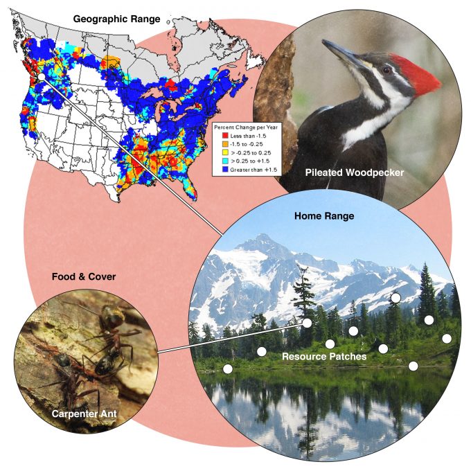
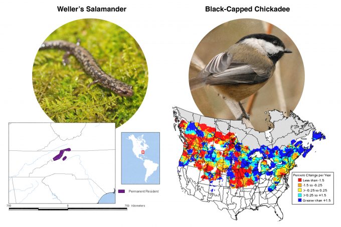
Many studies have been conducted to assess habitat selection by wildlife species. Johnson (1980) suggested that many species select habitat at four levels and called these levels, first-, second-, third-, and fourth-order selection (Figure 9.1). First order selection is selection of the geographic range. The geographic range defines, quite literally, where in the world this species can be found. In our example from figure 9.1, pileated woodpeckers are found in forests throughout the eastern and western North America. Considering two extremes underscores the significance of understanding first-order selection: Figure 9.2 shows geographic range maps for two species, Weller’s salamander, found in spruce forests above 1500 m (5000 feet) in the southern Appalachians, and black-capped chickadees found throughout the northern US and southern Canada. These two species have widely divergent geographic ranges and any monitoring protocols developed must consider these differences.
Consider the importance of populations of a species at the center vs the periphery of its geographic range. Populations at the periphery may be in lower quality habitat if either biotic or abiotic factors are limiting its distribution. But recall that environments are not static. They are constantly changing. Climate changes, earthquakes change the topography, some species arrive while others leave. It is those populations at the periphery of their geographic range that are on the front line of these changes. Hence although it may be tempting to think of these peripheral populations as somewhat expendable, they may be critical to population maintenance as large scale changes in habitat availability occur. Given the contemporary rate of climate change, these peripheral populations may be even more important over the next few hundred years (McArty 2001).
Although Johnson (1980) did not describe metapopulation distribution as a selection level, it is important to realize that within the geographic range, populations oftentimes are distributed among smaller, interacting sub-populations that contribute to overall population persistence. In this structure, defined as a metapopulation, the growth, extinction, and recolonization of and by sub-populations is an adaptation to habitat quality changes caused by iterative disturbance and regrowth. The distribution of the sub-populations is important to consider during development of a monitoring plan to ensure that not only the sub-populations are included in the monitoring framework, but suitable habitat patches not currently occupied, as well as the intervening matrix are also included.
Johnson (1980) described second-order selection as the establishment of a home range: the area that an individual or pair of individuals uses to acquire the resources that it needs to survive and reproduce. Not all species have established home ranges, but most do. Individuals which have nests, roosts, hibernacula, or other places central to their daily activities move in an area around that central place to acquire food, use cover, drink water, and raise young. Home ranges are not the same as territories. A territory is the space, usually around a nest, that an individual or pair defends from other individuals of the same species and occasionally other individuals of other species. Territories may be congruent with a home range, smaller (if just a nest site is defended), or may not be present at all.
Species with larger body mass need more energy to support that mass than smaller-bodied species. Herbivores tend to have smaller home ranges than carnivores of the same size, both because energy available to herbivores is more abundant and because with each increase in trophic level there is a decrease in energy availability. Home range sizes also vary among individuals within a species. Generally speaking, if food resources are less abundant or more widely distributed, home range size increases. But within a species the home range size has an upper limit that is governed by balancing energy input from food with energy loss by movement among food patches. For instance, Thompson and Colgan (1987) reported larger home ranges for American marten during years of low prey availability than in years of high prey availability. In this example, to ensure that observations of American marten are independent from one another, sample sites should be distributed in a manner that no individual marten is likely to visit more than one site. Because marten can be difficult to detect in some settings, however, sub-samples within sample sites may be used to ensure that the species is detected if it is present.
Third order selection is the use of patches within a home range where resources are available to meet an individual’s needs. Biologists often can delineate a home range based upon observed daily or seasonal movements of individuals going about their business of feeding, resting, and raising young. But this area is not used in its entirety. Rather there are some places within the home range that are used intensively and other parts of the home range that are rarely used (Samuel et al. 1985). Selection of these patches is assumed to represent the ability of the individual to effectively find and use resources that will allow it to survive and reproduce. Sampling in these patches can influence the detectability of a species to the extent that sampling says more about the habitat elements and resources important to the species of interest rather than a species’ density or abundance.
Fourth order selection is the selection of specific food and cover resources acquired from the patches used by the individual within its home range. Given the choice among available foods, a species should most often select those foods that will confer the greatest energy or nutrients to the individual. Which food or nest site to select is often a tradeoff among availability, digestibility, and risk of predation (Holmes and Schultz 1988). Factors that influence the selection of specific food and cover resources most often tend to be related to energetic gains and costs, but there are exceptions. The need for certain nutrients at certain times of the year can have little to do with energetics and much to do with survival and fitness. For instance, band-tailed pigeons seek a sodium source at mineral springs to supplement their diet during the nesting season (Sanders and Jarvis 2000).
Collectively, these levels of habitat selection influence the fitness of individuals, populations and species. Habitat quality is dependent not only on the food and cover resources but also the number of individuals in that patch. Many individuals in one patch means that there are fewer resources per individual. Habitat quality and habitat selection is density dependent. Hence sampling of habitat elements must consider the likely effects of population density on the probability of detecting a resource. Sampling browse in a forest with high deer densities will result in an estimate of browse availability only in relation to that population size, and not to the potential of the forest to provide browse biomass.
Remotely Sensed Data
Some information on habitat availability for selected species can be efficiently collected over large areas using remotely sensed data. In the very simplest form, maps allow users to better define their sampling framework by locating and delineating important areas and habitat types. Users can classify areas based on a variety of physiographic characteristics, and are able to document site-specific information, such as winter roosts, vernal pools, and breeding grounds. Data for maps can be based on a number of sources including aerial photographs, satellite imagery, orthophotos, or planimetric maps (Kerr 1986).
Aerial Photography
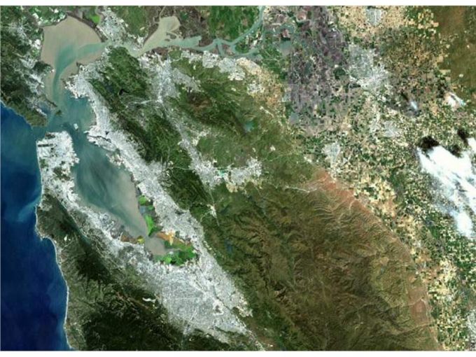
Monitoring and inventorying programs often use aerial photography for creating maps. Generally, these programs use aerial photos from scales of 1/2,000 to 1/60,000 for the purposes of classification and planning (Kerr 1986). Aerial photographs should not be considered as maps because they contain inherent degrees of radial and topographical distortions. Thus, aerial photographs must be corrected for geometric and directional inaccuracies. However, many Geographic Information Systems (GISs) are capable of correcting these problems. Orthophoto maps are commonly used for large-scale monitoring projects (covering 8,000-400,000 ha). These maps are corrected aerial photos with topographic information superimposed. If available, these types of data can be very useful during design of a sampling scheme. Aerial photography is usually available in black and white, true color, and color-infrared (Figure 9.3).
Color-infrared aerial photography is useful for identifying riparian vegetation and seasonally dominant vegetation (Cuplin 1986, Kerr 1986). The primary use of color infrared photographs is for analyzing and classifying vegetation types. This is because healthy green vegetation is a very strong reflector of infrared radiation and appears bright red on color infrared photographs. Often times, aerial photography is taken at different times in the year, allowing for seasonal comparisons of vegetation types (i.e., leaf-on and leaf-off photography). Yearly differences can be documented to describe changes in habitat area and composition over time.
Although aerial photography can be essential in creating maps for habitat types and area classification, the accuracy of these maps depends on photo interpretation by humans. Misclassification of habitat types is one common result of human error during photo interpretation. Consequently, although aerial photography is an indispensable tool for creating a sampling framework over large geographic areas, the accuracy, reliability, and usefulness of the map is influenced by the expertise of those responsible for interpreting and classifying the photography.
Satellite Imagery
Satellite imagery has become a popular method for describing gross vegetation types over large geographic areas (Figure 9.4). The majority of satellite imagery data comes from the LANDSAT program. The LANDSAT program refers to a series of satellites put into orbit around the earth to collect environmental data about the earth’s surface (Richards and Jia 1999). The U.S. Department of Interior and NASA initiated this program under the name Earth Resources Technology Satellites. Spatially, these data consist of discrete picture elements, referred to as pixels, and is radiometrically classified into discrete brightness levels (Richards and Jia 1999). This reflected light is recorded in different wavelength bands, the number of which depends on the type of sensor carried by the satellite. For instance, LANDSAT 7 was launched in April 1999 and carries the Enhanced Thematic Mapper Plus (ETM+), which produced data in 7 specific bands and 1 panchromatic band (Richards and Jia 1999).
The area each pixel covers on the ground is referred to as that image’s resolution. The pixel size for Landsat image data is typically 30 m2. Using the digital reflectance data, these images can be initially classified by humans, but later extrapolated through computer classification, to the rest of the image. Satellite imagery produces digital data, which carries the distinctive advantage of being able to be processed by computers that can distinguish small differences in color in a consistent, easily repeatable way.
There are, however, several drawbacks to using satellite imagery. In general, satellite imagery does not provide the detail that is found in aerial photography (Kerr 1986). Computer interpretation and classification often has difficulty in separating vegetation species or areas of the same reflectance. This may pose a problem if one is attempting to classify areas based on a species of plant. The scale of image resolution may not be sufficient to address the needs of the monitoring protocol. Although satellite imagery has proved useful for regional analyses (see Scott et al. 1993), the level of spatial detail and resolution may not be appropriate for small-scale monitoring programs.
Accuracy Assessment and Ground-truthing
The accuracy of satellite imagery depends on ground-truthing and subsequent accuracy assessment. The process of classifying such broad ranges of environmental features into specific, and often simplified, land use and land cover classes leads to inevitable errors in classification. Having a well-distributed grid of Global Positioning System(GPS) field surveys is a useful method for rectifying such problems. This process, ground-truthing, is an absolute necessity for any map, whether or not the map is based on satellite imagery or aerial photography. However, this method can be relatively expensive if there are a large number of ground points across an extensive geographic area. Recently, aerial videography has become a useful method for assessing the accuracy of Landsat imagery. This method consists of airborne video data systems that tag each frame of video with geographic coordinates from a GPS, providing a cost- and time-effective method for obtaining data on vegetative communities over large geographic areas (Graham 1993). This method can be combined with ground-truthing procedures, but allows for a decreased dependency on ground-based field surveys. These methods of accuracy assessment, and others like them, allow for rigorous statistical analyses to produce acceptably accurate land use and land cover maps. It is important to stress that to legitimately use and create accurate maps based on satellite imagery or aerial photography, monitoring protocols must incorporate ground-truthing and accuracy assessment.
Vegetation Classification Schemes
Vegetation classification is a common use of map data. Although vegetation can change over time and may not be a particularly useful means of stratifying samples, vegetation structure and composition are often highly related to a species occurrence or abundance. Biologists and managers often use a hierarchal approach to stratify vegetation types based on dominant and subdominant vegetation, landform, soil composition, or other factors that they deem pertinent (Kerr 1986). Once a classification criterion is determined, the landscape can be separated into discrete units so that samples can be distributed into an adequate number of habitat types which represent strata in a stratified random sample. Vegetation stratification can yield important information about the use of different types by a species. The Resource Inventory Committee of British Columbia has outlined a good approach to vegetation stratification (Robinson et al. 1996):
- Delineate the project area boundary.
- Conduct a literature review of the habitat requirements of the focal species. If there is enough available and accurate information on the habitat requirements of the species, then it may be possible to identify those vegetation components that relate to habitat quality. However, caution should be used when relying on habitat associations from previous studies since many studies may not be applicable to the region of study.
- Develop a system of habitat stratification that you expect will coincide with species habitat requirements.
- Use maps, aerial photographs, or satellite imagery to review and select sample units that are reflective of the study area.
- Evaluate the availability of each habitat strata within the study area. If there are any habitat types that are inaccessible, then no inferences can be made to similar habitat types throughout the project area.
Consistent Documentation of Sample Sites
To accurately monitor changes in habitat and populations, long-term monitoring protocols must emphasize a repeatable sampling scheme. Making inferences about a population from a sample taken over time depends on the ability of a protocol to re-sample and re-visit the same set of points from one year to the next. Monitoring protocols should incorporate consistent documentation of sample sites throughout the study area. This typically involves the use of GPSs, GISs, and other computer-based systems for data analysis, storage, and retrieval. GPS is a valuable tool for conducting field surveys and relocating sample sites. Using GPS, researchers can geo-reference sample site locations using latitude, longitude, or UTM coordinates. Along with GPS, careful notes should be taken on the location and description of sample sites. These notes should be reported in a consistent manner and held in office records. Data management and documentation remains a critical component of project supervision. It is vitally important that there is proper documentation and storage of sample site locations for ensuring the long-term and repeatable success of monitoring protocols.
Ground Measurements of Habitat Elements
Oftentimes a monitoring framework will be based on remotely sensed data as a first coarse-scale approach to documenting change followed by more detailed ground-based sampling. Changes in resource availability for species often are predicted using measurements of habitat elements and habitat types. Habitat measurements include abiotic and biotic features such as rock, soil, elevation, vegetation types, snags, ground cover, and litter. These data apply to a specific habitat type, which is defined as an area that is characterized by consistent abiotic and biotic features (Jones 1986). To assess habitat availability, a number of measurements are documented at various scales and include (Jones 1986):
- size of sites (area);
- location and position of habitat sites, including distance between habitat sites and heterogeneity within an area;
- edge influences created by habitat size interfaces and ecotones;
- temporal availability of habitat sites.
These data are collected over various scales; however, the relevant scale at which to collect and interpret these data will be defined by the organism (see previous section).
Information that relates to the abiotic or biotic influences on the species is considered a habitat element or component (Jones 1986). These elements can be highly significant measurements in terms of the distribution, fitness, and stability of a population throughout their range. Habitat elements are characterized both spatially and temporally, and can represent an entire habitat type or a specific area occupied by the species. Examples of abiotic and biotic data that are typically included are described by a number of authors: Cuplin 1986, Cooperrider 1986, Jones 1986 (Table 9.1):
| Habitat Feature | Habitat Components |
| Landform and physical features | Average elevation, slope, and aspect
Average surface rock cover, talus and rock outcrop abundance and size Soil depth and composition Vertical and horizontal heterogeneity of soils and rocks |
| Vegetation-derived features | Average leaf and litter cover per unit area
Snag density and size Dead and down woody debris Average height, density, and composition of vegetation types Vertical and horizontal heterogeneity of litter, snags, and live vegetation |
| Aquatic physical features | Streamflow pattern (riffles, pools, glides and cascades)
Streamflow volume Stream width, depth and gradient Water temperature Turbidity Surface acreage Stream channel stability |
The measurement and interpretation of habitat elements is central to understanding current conditions and desired future conditions in patches and landscapes. In the subsequent sections we describe a few simple techniques for measuring the availability of key habitat elements, but more comprehensive information on field sampling of habitat elements can be found in Bookhout (1994), James and Shugart (1970), Hays et al. (1981), and Noon (1981).
Methods for Ground-Based Sampling of Habitat Elements
Some habitat elements are particularly important to many species depending on their size, distribution and abundance. These include: percent cover, height, density, and biomass of trees, shrubs, grasses, forbs, and dead wood. Other habitat elements are associated with only a few species, such as stream gradients (e.g., beaver; Allen 1983) and tree basal area (e.g., downy woodpecker, Schroeder 1982). The following constitutes suggestions for an exercise that will train you in some of the more common habitat sampling methods:
Visit two areas with very different management histories such as a recent clearcut and an unmanaged forest. First, compare habitat elements between the two stand types. Then choose a particular organism and, using life history information, a habitat suitability index model, and a geographic information system, assess the habitat quality of each for that species.
Random Sampling
Probably the most important part of sampling habitat is to sample randomly within the area of interest (stand, watershed, stream system, etc.). Systematic or subjective sampling can introduce bias into your estimates and lead to erroneous conclusions. In this example you will be sampling two forest stands, but it could be wetlands, prairies, or any other unit of land or water. Within your stand you should collect a random sample of data describing the habitat elements. For the purposes of this exercise, you will collect data from three or more randomly located points in each stand.
- Using a random numbers table (nearly all statistics books have these) first select a 3-digit number that is a compass bearing (in degrees) that will lead you into the stand. If the number that you select does not lead you into your stand then select another number until you have a bearing that will work.
- Select another 3-digit number that is a distance in meters. Using your compass to establish the bearing and either a 30-m tape measure or pacing, walk the randomly selected distance in the direction of the assigned bearing and establish a sample point. You will collect habitat data at this point. Once you have completed collecting data at this point, you repeat the process of random number selection three or more times in this stand and then three or more times in the second stand.
Vegetation Sampling
Measuring density
One of the most common habitat elements that you will measure is density of items, usually trees, snags, logs, shrubs, or other plants. Density is simply a count of the elements over a specified area. Counting individual plants on plots delineated by a sampling frame is the most commonly used approach to estimate the frequency or density of plant populations. Measurements of plant biomass also can be obtained from the dry weights of vegetation clipped on plots having standardized heights, as well as width and length. Standardized photographic methods (i.e., photoplots) can be used to capture a visual record of a sampling unit that is useful for monitoring studies (Elzinga et al. 1998).
Data collected from plots are affected by the size and shape of the sampling unit. Square plots, known as “quadrats”, and circular plots have smaller boundary/interior ratios compared to rectangular shapes of equal area. In heterogeneous habitats, data collected on long plots often have been found to have lower statistical variance than data from compact plots of the same total area (Krebs 1989).
The optimum size and shape of a plot will differ according to plant life-form, environmental conditions, and survey objectives. Typically, the optimum plot configuration will be one that provides the greatest statistical precision (i.e., lowest standard error) for a given area sampled. Several investigators have developed approaches for determining the most appropriate plot size and shape for a particular population survey (Hendricks 1956, Weigert 1962). Krebs (1989) provided a useful review of standardized plot methods.
When estimating the density of trees, you usually will count all the trees in a circular plot, usually 0.04 ha (0.1 acre) in size. Saplings and tall shrubs are usually measured in a 0.004-ha (0.01-acre) plot. Small shrubs and tree seedlings are usually measured in a 0.0004-ha (0.001-acre) plot.
- From plot center, measure out in each cardinal direction (N, E, S, W) 11.3 m (37.2 feet) (the radius of a 0.04 ha [0.1-acre] plot). Mark these places with flagging.
- Using a diameter tape or a Biltmore stick, measure the diameter at 1.3 m (4.5 feet) above ground of all live trees in the plot that are > 15 cm (6 inches) in diameter at breast height (dbh) and record the species of each tree. Repeat this procedure for all dead trees > 15 cm dbh. Expand this sample to a ha (or acre) by multiplying the estimates by the proper conversion factor, in this case using 25/1 converts our number to a per ha estimate (10/1 will generate a per acre estimate). This procedure, with the appropriate conversion factors, can be repeated for smaller plot sizes to estimate more tediously sampled habitat components such as seedling numbers.
Estimating Percent Cover
Use your four 11.3-m (37.2-foot) radii as transects, by walking along each and stopping at five equidistant points to estimate canopy cover. There are a number of techniques available to estimate canopy cover including moosehorns (Garrison 1949) and densitometers (Lemmon 1957). A simple approach to estimating cover is to estimate the presence or absence of vegetation using a sighting tube (a piece of PVC pipe with crosshairs) (James and Shugart 1970). At each of the 20 points on your transects, look directly up and see if the crosshairs intersect vegetation (if so record a ‘1’) or sky (if so, record a ‘0’). Repeat this at each of the five points on each of the four transects. Tally the number of ‘1’s recorded from these points. Divide by 20 to estimate the proportion of the plot covered by vegetation. A similar approach to estimating cover can be used by looking down rather than up, but estimates of ground covered by grasses and forbs often use somewhat different techniques. One method of measuring ground cover for a plant species is to calculate the percentage of points in contact with the target species from a standardized arrangement of points on the sampling unit. The technique utilizes marks at fixed intervals along a tape, or pins held along a linear frame positioned above the sampling unit (i.e., point frame). Points are particularly useful for estimating the cover of short grasses, dense patches of forbs, and other low plant species. Bonham (1983) reviews several types of simple apparati to standardize point observations and greatly improve the precision of cover measurements.
Ground and shrub cover can also be measured using a fiberglass measuring tape stretched tautly between two end poles. The surveyor proceeds along the tape, recording each point where the tape first intercepts the vertical plane of any above-ground plant part of the target species, and then the point where interception with the target species is interrupted. Cover is estimated as a percentage of the total length of tape intercepting the target species. Interception points can be reliably observed along the tape to approximately eye-level; a staff or contractors level held vertically and moved along the tape by the surveyor can extend the effective height of measurements to 4 m or more. The position of the end poles should be permanently monumented to ensure re-measurements are reliably positioned.
Estimating tree height
Use a clinometer with a percent scale (look through the view finder and you should see two scales, with units given on them if you look straight up or straight down).
- Walk 30 m (100 feet) from the base of the tree or other object that you wish to measure.
- Looking through the view finder, align the horizontal line in the view finder with the top of the tree. Record the number on the percent scale (top).
- Looking through the view finder, align the horizontal line in the view finder with the base of the tree. Record the number on the percent scale (bottom).
- If the top number is positive and the bottom number is negative (< 0) then add the absolute values of these two numbers together to estimate height in feet.
- If the top number is positive and the bottom number is also positive (> 0), then subtract the absolute value of the bottom number from the top number to estimate height in feet.
Estimating basal area
Basal area is the cross-sectional area of all woody stems at 1.3 m (4.5 feet) above ground. It is a measure of tree dominance on a site. The higher the basal area, the greater the dominance by trees. There are two ways to estimate basal area. First, you can use your estimates of dbh from your sample of trees (see estimating density, above) to calculate the area of each stem (A=3.1416*r2, where r = dbh/2). By summing the areas on a 0.04-ha (0.1-acre) plot and then multiplying the total by 25, you arrive at an estimate of basal area per hectare (multiply by 10 to estimate basal area per acre).
Alternatively, you can use a wedge prism (Figure 9.5) using a plotless method for estimating basal area. Holding the prism over the plot center (do not stand at the center), look at a tree through the prism. If the image that you see through the prism is connected to the image of the tree outside of the prism then tally the tree and record its species. If the image that you see through the prism is disconnected from the image outside the prism, then do not record the tree. Moving in a circle around the prism that you continue to hold over plot center, record all trees that have the prism image connected to the image outside of the prism regardless of whether they fall in the 0.04-ha (0.1-acre plot) or not. Tally the number of trees that were recorded. Generally you will use a 10-factor prism, that is, each tallied tree represents 10 other trees per acre. Multiply the number of trees tallied by 10 and this estimates the basal area in square feet per acre for this site. Other factor prisms do exist, however, and may be more appropriate for your survey depending on the specific characteristics of the habitat being sampled (Wensel et al. 1980).
Another class of “plotless” techniques utilizes measurements to describe the spacing of individuals in an area to estimate population density. Commonly referred to as “Distance Methods”, these techniques are founded on the assumption that number of individuals in a population can be determined by measuring the average distance among individuals, or between individuals and randomly selected points. Two of the most widely used techniques include the Point-Centered Quarter Method (Cottam and Curtis 1956) and the Wandering-Quarter Method (Cantana 1963). Distance methods have been commonly used for vegetation surveys, and are easily adapted to inventories of rare plants or other sessile organisms. Collecting data for surveys based on distance methods may have some practical advantages over plots or transects. First, distance methods are not susceptible to counting errors that often occur near plot boundaries, thus may yield more accurate density estimates. Secondly, the time and effort to attain an adequate sample of distance measurements in an area often is less than that required to search for every target organism on a plot, thus increasing the efficiency of the survey. Cottam and Curtis (1956) recommended a minimum of 20 measurements for estimating population density or abundance using Point-Centered Quarter Method. However, it is always prudent to assess the adequacy of the sample size empirically using widely available formulas (Bonham 1989).
Sampling Dead wood
Dead wood has been recognized as a habitat element important to many species (McComb 2007). There are a number of methods for sampling dead wood, but the most comprehensive uses line intercept sampling to generate estimates of a variety of dead wood characteristics (Harmon and Sexton 1996). The line transects often radiate out from a plot center and the diameter of logs on which they fall is measured at the point of intersection. Usually an estimate of decay class (1-5) is also made (McComb 2007). Diameters of elliptically-shaped logs should be measured in two dimensions and then averaged to get a single value. These measurements are then used. Volume, projected area, and surface area of small and large CWD can be calculated using the following equations (Marshall et al. 2000; Marshall et al. 2003):
- Volume/ha (m3/ha) = (π2/(8*transect length)) * ∑(log diameters2)
- Total projected area/ha (m2/ha) = ((50* π)/transect length) * ∑(log diameters)
- Total surface area (m2/ha) = ((50* π2)/transect length) * ∑(log diameters),
where transect length is in meters and log diameter is in centimeters.
Estimating biomass
Biomass of vegetation is usually estimated to provide information on winter food availability for herbivores. A number of species, including deer, moose, elk, and hare, depend most on these browse resources after the vegetation senesces. Herbivores usually will only eat woody growth resulting from the most recent growing season, and during winter, this includes the twigs and buds, but not leaves.
Within a 1.1-m (3.7-foot) radius plot, use clippers to clip all of the twigs within the plot that have resulted from the most recent growing season. Remove and discard the leaves and place the twigs in a bag. Return to the lab and weigh the bag with the twigs. Remove the twigs and weigh the empty bag. Subtract the bag weight from the bag + twigs weight to estimate biomass per 0.0004-ha (0.001-acre) plot. Multiply this number by 2500 to estimate biomass (kg) per ha (or 1000 to generate a per acre estimate). Because the proportion of the food biomass composed of water can vary from one period of the growing season to the next and from one year to the next, usually the sampled are oven dried and then weighed to standardize estimates of biomass.
Using Estimates of Habitat Elements to Assess Habitat Availability
The aggregate data on habitat element abundance, sizes, and distribution can now be used to estimate habitat availability. Using table 9.2 and the downy woodpecker as an example (if you are carrying out this exercise, you can use your own numbers and species information from your field samples and research), consider how you would interpret these data. DeGraaf and Yamasaki (2001) described habitat for downy woodpeckers as: ”…woodlands with living and dead trees from 25-60 cm dbh; some dead or living trees must be greater than 15 cm dbh for nesting.” Although both sites contain trees and snags of sufficient size, the canopy cover data in table 9.2 would suggest that the clearcut is not functioning as a woodland. Thus, we would probably not consider it suitable habitat for downy woodpeckers (though they certainly do use snags in openings at times). Similar descriptions of habitat are available for many species in North American and Europe sp this type of subjective assessment of habitat availability can be easily accomplished.
| Clearcut | Mature Forest | |
| Trees > 15 cm/ha | 3 (0-6) | 308 (234-412) |
| Snags > 15 cm/ha | 1 (0-2) | 22 (4-43) |
| Basal area/ha | 2.4 (0-3) | 16 (12-18) |
| Canopy cover (%) | 4 (0-7) | 95 (90-100) |
| Canopy height (m) | 23 (18-34) | 27 (23-33) |
| Browse (kg/ha) | 1234 (554-2600) | 387(122-788) |
Using Estimates of Habitat Elements to Assess Habitat Suitability
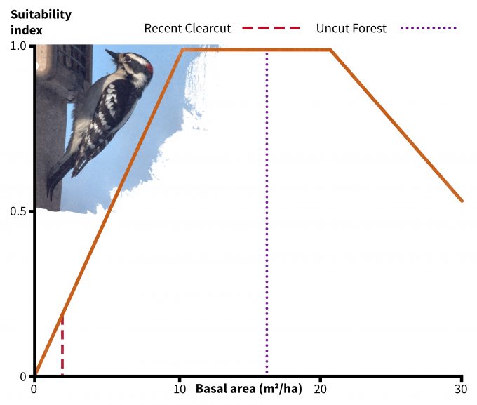
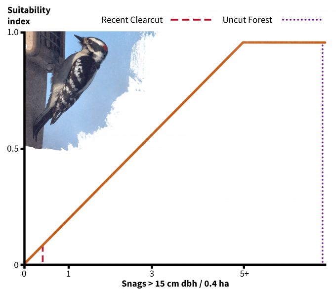
In addition to using your data to understand if a site might be used by a species, habitat suitability index models have been developed to understand if some sites might provide more suitable habitat than others (e.g., Schroeder 1982). Very few of these models have been validated, especially not using fitness as a response variable. Nonetheless they do represent hypotheses based on the assumption that there is a positive relationship between the index and habitat carrying capacity. In the case of the downy woodpecker, its habitat suitability is based on two indices: tree basal area (Figure 9.6) and density of snags > 15 cm dbh (Figure 9.7). Considering first the uncut stand Table 9.2), note that there is an average of 16 m2/ha of basal area and 22 snags per ha (8.8 per 0.4 ha). The corresponding suitability index score for each variable is 1.0 and the overall habitat suitability is calculated (in this case) as the minimum of the two values. Hence this should be very good habitat for downy woodpeckers. In the recent clearcut however, the suitability index for snags is approximately 0.1 and for basal area is approximately 0.2. Hence the overall suitability in the recent clearcut for this species is 0.1; according to this index, it is both unsuitable in general and much less suitable relative to the uncut stand. Further, in the recent clearcut, snag density, which has the lowest index score, is the factor most limiting habitat quality for downy woodpeckers. The best way to use these types of models is to compare the habitat suitability of one site to another rather than as definitive data pertinent to species abundance, density, or fitness. It is also not justifiable to use habitat suitability scores as the basis for value judgments; indeed, if we were use this technique to assess habitat suitability for snowshoe hares then we might find the recent clearcut to be much better habitat.
Assessing the Distribution of Habitat Across the Landscape
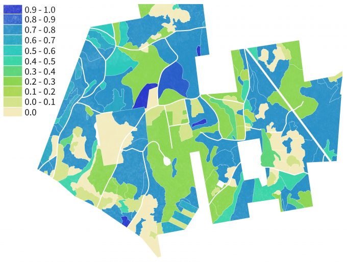
It is often as imtortant to know if patches are suitable habitat for a species and how they are arranged on a landscape. In figure 9.8, a 490-ha forest has been broken into habitat types based on overstory cover and stand structure. Field samples were taken at 117 points distributed across the forest and habitat elements were sampled at each point. Habitat suitability index values are then calculated at each point and extrapolated to the habitat types as portrayed in this figure to illustrate how habitat availability for a species can be displayed over a landscape. A different pattern would emerge for other species using this same approach, and these would have to be overlain on patches used as the basis for management. In addition to synthesizing monitoring information to display changes in spatial patterns, these types of maps can guide planning for management activities in order to achieve habitat patterns leading to a desired future condition for the landscape.
Linking Inventory Data to Satellite Imagery and GIS
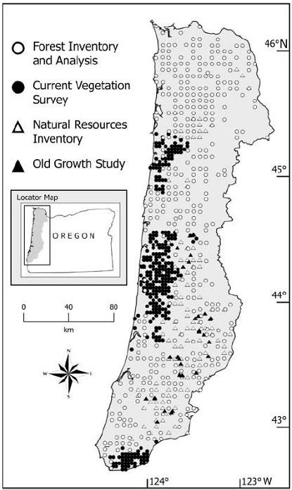
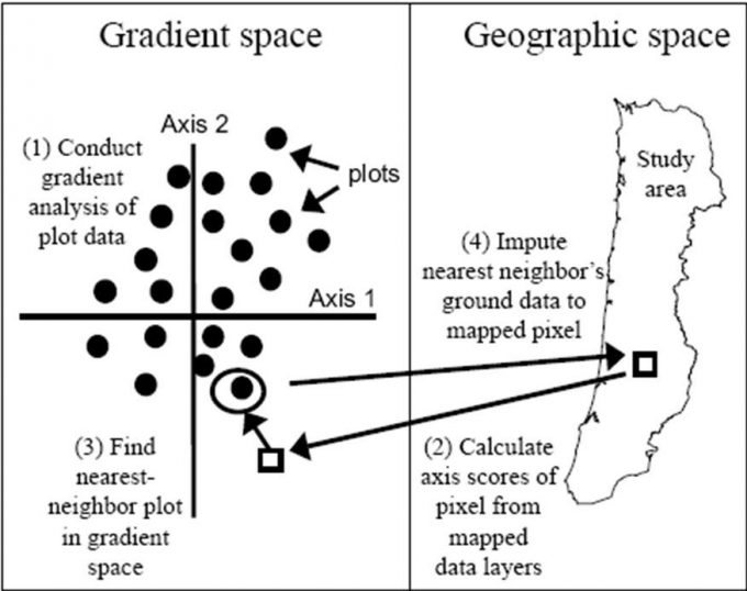
Ohmann and Gregory (2002) described a technique called gradient nearest neighbor (GNN) approaches to populate raster cells in satellite imagery with ground plot data (Figure 9.9). They used direct gradient analysis and nearest-neighbor imputation to ascribe detailed ground attributes of vegetation to each pixel in a digital landscape map (Figure 9.10). The gradient nearest neighbor method integrates vegetation measurements from regional grids of field plots, mapped environmental data, and Landsat Thematic Mapper (TM) imagery (Ohmann and Gregory 2002). The accuracy of maps created with this approach is normally questioned, but at the regional level, mapped predictions represent the variability in the sample data very well and predict area by vegetation type accurately in many forests where the approach has been tested. For instance, prediction accuracy for tree species occurrence and several measures of vegetation structure and composition was good to moderate in the Oregon Coast Range (Ohmann and Gregory 2002). Vegetation maps produced with the gradient nearest neighbor method are often used for regional-level monitoring, planning, and policy analysis. Their utility decreases as they are used over smaller spatial scales.
Results of the maps generated using the GNN approach can then be reclassified in a nearly infinite number of ways to represent habitat availability for various species over large areas (figure 9.11). With repeated monitoring of ground plots and synchronous acquisition of satellite image data, new projections of habitat availability can be developed over time to understand trajectories of change. In addition, by linking the ground plot data to vegetation growth models, changes in vegetation structure and composition and resulting habitat can be projected into the future under various assumptions regarding land use, natural disturbances or other environmental stresses (Spies et al. 2007).
Measuring Landscape Structure and Change
In addition to assessing habitat elements at various spatial scales over space and time, the pattern of patches across landscapes can be monitored. The assumption often made by landscape ecologists is that pattern influences process and processes create patterns. Consequently, knowledge of aspects of landscape patterns such as characteristics of patches (size, shape, edges, etc.) and among patches (richness, diversity, arrangement) can be informative when inferring how processes might be influenced by changes in landscape pattern. One often-used tool used to generate measurements of landscape pattern is FRAGSTATS (McGarigal et al. 2002). FRAGSTATS quantifies the extent and configuration of patches in a landscape. The user must define the basis for the analysis, including the extent (outer bounds) and grain (the finest level of detail) in the landscape. All patches in a landscape must be classified in a manner that is logical to the objectives of the analysis (e.g., related to habitat for a species or group of species). FRAGSTATS computes 3 groups of metrics. For a given landscape mosaic, FRAGSTATS computes several metrics for: (1) each patch in the mosaic; (2) each patch type (class) in the mosaic; and (3) the landscape mosaic as a whole (McGarigal et al. 2002. These metrics can easily become the basis for long term monitoring to assess changes in landscape patterns and allow inference to changes in landscape processes.
Summary
Effectively sampling habitat within a monitoring framework requires that the key habitat elements for the species (or species’) be defined. Habitat is a species-specific concept so unless monitoring is focused on habitat types (a biophysical classification of the environment), then a set of habitat elements must be identified as important to one of four levels of habitat selection: geographic range, home range, resource patches or habitat resources. Sampling these habitat elements must consider these scales of habitat selection when defining the grain and extent of a monitoring framework for the species of interest. Often remotely sensed data are used as a first assessment of habitat patches, but ground plot data are usually stratified by patch types identified from remotely sensed data. Ground plot data can provide more detailed information on the availability of habitat elements when extrapolated to specific patch types, or can be used to populate a GIS layer using gradient nearest neighbor approaches. Remotely sensed data, ground plot data and GIS layers interpreted as habitat for the species of interest can all be used to monitor changes over time in habitat availability for a species. Similarly, changes in the pattern of landscape structure can be assessed over time to understand how changes in pattern might influence key ecological processes on the landscape. FRAGSTATS is a commonly used tool to conduct such assessments.
References
Allen, A.W. 1983. Habitat suitability index models: beaver. USDI Fish and Wildlife Service FWS/OBS-82/10.30 (Revised). Washington, DC
Barrett, R.H. and H. Salwasser. 1982. Adaptive management of timber and wildlife habitat using DYNAST and wildlife-habitat relationships models. Pages 350-365 IN Proceedings of the Western Assoc. Fish and Game Agencies.
Bonham, C.D.1983. Range vegetation classification. Rangelands 5:19-21.
Bonham, C.D. 1989. Measurements of terrestrial vegetation. John Wiley, New York, New York, USA.
Bookhout, T.A. 1994. Research and management techniques for wildlife and habitats, 5th ed. The Wildlife Society, Bethesda, MD.
Cantana, H.J. 1963. The wandering quarter method of estimating population density. Ecology 44: 349-360.
Cody, M.L. 1985. Habitat selection in birds. Academic Press, New York, New York.
Cooperrider, A.Y., R.J. Boyd, and H.R. Stuart, eds. Inventory and monitoring of wildlife habitat. USDI BLM, Service Center. Denver, Co. 858pp.
Cottam, G., and J. T. Curtis. 1956. The use of distance measures in phytosociological sampling. Ecology 37:451-460.
Cuplin, P., W.S. Platts, O. Casey, amd R. Masiton. 1985. A comparison of riparian area ground data with large scale airphoto interpretation. Pages 67-68. In: R.R. Johnson, C.D. Ziebell, D.R. Patton, P.F. Folliott, and R.H. Hamre, tech. coords. Riparian ecosystems and their management: reconciling conflicting uses: Proceedings, first North American riparian conference. USDA Forest Service General Technical Report RM-120.
DeGraaf, R.M. and M. Yamasaki. 2001. New England wildlife: habitat, natural history, and distribution. Univ. Press of New England, Hanover, NH.
Garrison, G.A. 1949. Uses and modifications for the “moosehorn” crown closure estimator. Journal of Forestry 47:733-735.
Garshelis, D.L. 2000. Delusions in habitat evaluation: measuring use, selection, and importance. Pages 111-153 in L. Boitani and T.K. Fuller, editors. Research techniques in animal ecology: controversies and consequences. Columbia University Press, New York, New York, USA.
Graham, L.A. 1993 Airborne video for near real-time vegetation mapping Journal of Forestry 90(12): 16-21.
Harmon, M.E., and J. Sexton. 1996. Guidelines for measurements of woody detritus in forest ecosystems. US LTER Network Office, University of Washington, College of Forest Resources. US LTER Publication 20.
Hays, R.L., C. Summers, and W. Seitz. 1981. Estimating wildlife habitat variables. USDI Fish and Wildlife Service FWS/OBS-81/47.
Hendricks, W.A. 1956. The mathematical theory of sampling. The Scarecrow Press, New Brunswick, N. J. 364pp.
Holmes, R.T., and J.C. Schultz. 1988. Food availability for forest birds: effects of prey distribution and abundance on bird foraging. Canadian Journal of Zoology 66:720-728.
James, F.C., and H.H. Shugart, Jr. 1970. A quantitative method of habitat description. Amer. Birds 24:727-236.
Johnson, D.H. 1980. The comparison of usage and availability measurements for evaluating resource preference. Ecology 61:65–71.
Jones, K. B. 1986. Data types. Pages 11-28 in A.Y. Cooperrider, R.J. Boyd, and H.R. Stuart, editors. Inventory and monitoring of wildlife habitat. USDI BLM, Service Center. Denver, Co. 858pp.
Kerr, R.M. 1986. Habitat mapping. Pages 49-72 In A.Y. Cooperrider, J.B. Raymond, and H.R. Stuart, editors. Inventory and monitoring of wildlife habitat. USDI BLM, Service Center. Denver, Co. 858pp.
Krebs, C.J. 1989. Ecological methodology. Harper Collins, New York, New York. 654pp.
Lemmon, P.E. 1957. A new instrument for measuring forest canopy overstory density. Journal of Forestry 55:667-638
Lowe, W.H., and D.T. Bolger. 2002. Local and landscape-scale predictors of salamander abundance in New Hampshire headwater streams. Conserv. Biol. 16:183-193.
Marshall, P.L., G. Davis, V.M. LeMay. 2000. Using line intersect sampling for coarse woody debris. BC Forest Service, Forest Research Technical Report TR-003. 34 pp.
Marshall, P.L., G. Davis, S.W. Taylor. 2003. BC Forest Service, Forest Research Extension Note EN-012. 10pp.
McCarty, J.P. 2001. Ecological consequences of recent climate change. Conservation Biology 15: 320–331.
McComb, B.C. 2007. Wildlife habitat management: Concepts and applications in forestry. Taylor and Francis Publishers, CRC Press, Boca Raton, FL. 319pp.
McGarigal, K., S.A. Cushman, M.C. Neel, and E. Ene. 2002. FRAGSTATS: Spatial Pattern Analysis Program for Categorical Maps. Computer software program produced by the authors at the University of Massachusetts, Amherst.
Noon, B.R. 1981. Techniques for sampling avian habitats. Pages 41-52 In D.E. Capen, editor. The use of multivariate statistics in studies of wildlife habitat. USDA Forest Service General Technical Report RM-87.
Ohmann, J.L. and M.J. Gregory. 2002. Predictive mapping of forest composition and structure with direct gradient analysis and nearest neighbor imputation in coastal Oregon, USA. Canadian Journal of Forest Research. 32:725-741.
Pulliam, H.R. 1988. Sources, sinks, and population regulation. American Naturalist 132:652-661.
Richards, J.A., and X. Jia. 1999. Interpretation of hyperspectral image data. Pages 313-337 in Remote sensing digital image analysis: an introduction. Springer, Publ., New York.
Robinson, C.L.K., D. E. Hay, J. Booth and J. Truscott. 1996. Standard methods for sampling resources and habitats in Coastal Subtidal Regions of British Columbia: Part 2 – Review of Sampling with Preliminary Recommendations. Canadian Technical Report of Fisheries and Aquatic Sciences 2119. Fisheries and Oceans Canada.
Samuel, M.D., D.J. Pierce, and E.O. Garton. 1985. Identifying areas of concentrated use within the home range. Journal of Animal Ecology 54:711-719
Sanders, T.A. and R.L. Jarvis. 2000. Do band-tailed pigeons seek a calcium supplement at mineral sites? Condor 102: 855-863
Schroeder, R.L. 1982. Habitat suitability index models: Downy woodpecker. USDI Fish and Wildlife Service FWS/OBS-82/10.38.
Scott, J.M., F. Davis, B. Csuti, R. Noss, B. Butterfield, C. Groves, H. Anderson, S. Caicco, F. D’Erchia, T.C. Edwards, Jr., J. Ullirnan, and R.G. Wright. 1993. Gap analysis: a geographic approach to protection of biological diversity. Wildlife Monographs 123.
Spies, T.A., B.C. McComb, R. Kennedy, M. McGrath, K. Olsen, R. J. Pabst. 2007. Potential effects of forest policies on biodiversity in a multi-ownership province. Ecological Applications 17:48-65.
Thompson, I.D. and P.W. Colgan. 1987. Numerical responses of marten to a food shortage in north-central Ontario. Journal of Wildlife Mangement 51:824-835.
Vesely, D. and W.C. McComb. 2002. Terrestrial salamander abundance and amphibian species richness in headwater riparian buffer strips, Oregon Coast Range. Forest Science. 48: 291-298
Wecker, S.C. 1963. The role of early experience in habitat selection by the prairie deer mouse, Peromyscus maniculatus bairdi. Ecological Monographs 33:307-325.
Wensel, L.C., J. Levitan, and K. Barber. 1980. Selection of basal area factor in point sampling. Journal of Forestry 78: 83–84.
