11 Data Analysis in Monitoring
Plant and animal data come in many forms including indices, counts, and occurrences. The diversity of these data types can present special challenges during analysis because they can follow different distributions and may be more or less appropriate for different statistical approaches. As an additional complication, monitoring data are often taken from sites that are in close proximity or surveys are repeated in time, and thus special care must be taken regarding assumptions of independency. In this chapter we will discuss some essential features of these data types, data visualization, different modeling approaches, and paradigms of inference.
This chapter is designed to help you gain bio-statistical literacy and build an effective framework for the analysis of monitoring data. These issues are rather complex, and as such, only key elements and concepts of effective data analysis are discussed. Many books have been written on the topic of analyzing ecological data. Thus, it would be impossible to effectively cover the full range of the related topics in a single chapter. The purpose, therefore, of the data analysis segment of this book is to serve as an introduction to some of the classical and contemporary techniques for analyzing the data collected by monitoring programs. After reading this chapter, if you wish to broaden your understanding of data analysis and learn to apply it with confidence in ecological research and monitoring, we recommend the following texts that cover many of the classical approaches: Cochran (1977), Underwood (1997), Thompson et al. (1998), Zar (1999), Crawley (2005, 2007), Scheiner and Gurevitch (2001), Quinn and Keough (2002), Gotelli and Ellison (2004), and Bolker (2008). For a more in-depth and analytical coverage of some of the contemporary approaches we recommend Williams et al. (2002), MacKenzie et al. (2006), Royle and Dorazio (2008) and Thomson et al. (2009).
The field of data analysis in ecology is a rapidly growing enterprise, as is data management (Chapter 10), and it is difficult to keep abreast of its many developments. Consequently, one of the first steps in developing a statistically sound approach to data analysis is to consult with a biometrician in the early phases of development of your monitoring plan. One of the most common (and oldest) lamentations of many statisticians is that people with questions of data analysis seek advice after the data have been collected. This has been likened to a post-mortem examination (R.A. Fisher); there is only so much a biometrician can do and/or suggest after the data have been collected. Consulting a biometrician is imperative in almost every phase of the monitoring program, but a strong understanding of analytical approaches from the start will help ensure a more comprehensive and rigorous scheme for data collection and analysis
Data Visualization I: Getting to Know Your Data
The initial phase of every data analysis should include exploratory data evaluation (Tukey 1977). Once data are collected, they can exhibit a number of different distributions. Plotting your data and reporting various summary statistics (e.g., mean, median, quantiles, standard error, minimums, and maximums) allows the you to identify the general form of the data and possibly identify erroneous entries or sampling errors. Anscombe (1973) advocates making data examination an iterative process by utilizing several types of graphical displays and summary statistics to reveal unique features prior to data analysis. The most commonly used displays include normal probability plots, density plots (histograms, dit plots), box plots, scatter plots, bar charts, point and line charts, and Cleveland dotplots (Cleveland 1985, Elzinga et al. 1998, Gotelli and Ellison 2004, Zuur et al. 2007). Effective graphical displays show the essence of the collected data and should (Tufte 2001):
- Show the data,
- Induce the viewer to think about the substance of the data rather than about methodology, graphic design, or the technology of graphic production,
- Avoid distorting what the data have to say,
- Present many numbers in a small space,
- Make large data sets coherent and visually informative,
- Encourage the eye to compare different pieces of data and possibly different strata,
- Reveal the data at several levels of detail, from a broad overview to the fine structure,
- Serve a reasonably clear purpose: description, exploration, or tabulation,
- Be closely integrated with the numerical descriptions (i.e., summary statistics) of a data set.
In some cases, exploring different graphical displays and comparing the visual patterns of the data will actually guide the selection of the statistical model (Anscombe 1973, Hilborn and Mangel 1997, Bolker 2008). For example, refer to the four graphs in Figure 11.1. They all display relationships that produce identical outputs if analyzed using an ordinary least squares (OLS) regression analysis (Table 11.1). Yet, whereas a simple regression model may reasonably well describe the trend in case A, its use in the remaining three cases is not appropriate, at least not without an adequate examination and transformation of the data. Case B could be best described using a logarithmic rather than a linear model and the relationship in case D is spurious, resulting from connecting a single point to the rest of the data cluster. Cases C and D also reveal the presence of outliers (i.e., extreme values that may have been missed without a careful examination of the data). In these cases, the researcher should investigate these outliers to see if their values were true samples or an error in data collection and/or entry. This simple example illustrates the value of a visual scrutiny of data prior to data analysis.
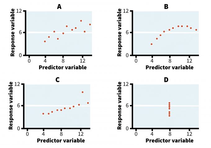
| A | B | C | D | Analysis output | ||||||||
| X | Y | X | Y | X | Y | X | Y | N = 11
Mean of Xs = 9.0 Mean of Ys = 7.5 Regression line: Y = 3 + 0.5X Regression SS = 27.50 r = 0.82 R2 = 0.67 |
||||
| 10.0 | 8.04 | 10.0 | 9.14 | 10.0 | 7.46 | 8.0 | 6.58 | |||||
| 8.0 | 6.95 | 8.0 | 8.14 | 8.0 | 6.77 | 8.0 | 5.76 | |||||
| 13.0 | 7.58 | 13.0 | 8.74 | 13.0 | 12.74 | 8.0 | 7.71 | |||||
| 9.0 | 8.81 | 9.0 | 8.77 | 9.0 | 7.11 | 8.0 | 8.84 | |||||
| 11.0 | 8.33 | 11.0 | 9.26 | 11.0 | 7.81 | 8.0 | 8.47 | |||||
| 14.0 | 9.96 | 14.0 | 8.10 | 14.0 | 8.84 | 8.0 | 7.04 | |||||
| 6.0 | 7.24 | 6.0 | 6.13 | 6.0 | 6.08 | 8.0 | 5.25 | |||||
| 4.0 | 4.26 | 4.0 | 3.10 | 4.0 | 5.39 | 19.0 | 12.50 | |||||
| 12.0 | 10.84 | 12.0 | 9.13 | 12.0 | 8.15 | 8.0 | 5.56 | |||||
| 7.0 | 4.82 | 7.0 | 7.26 | 7.0 | 6.42 | 8.0 | 7.91 | |||||
| 5.0 | 5.68 | 5.0 | 4.74 | 5.0 | 5.73 | 8.0 | 6.89 | |||||
The fact that, under some circumstances, visual displays alone can provide an adequate assessment of the data underscores the value of visual analysis to an even greater extent. A strictly visual (or graphical) approach may even be superior to formal data analyses in situations with large quantities of data (e.g., detailed measurements of demographics or vegetation cover) or if data sets are sparse (e.g. in the case of inadequate sampling or pilot investigations). For example, maps can be effectively used to present a great volume of information. Tufte (2001) argues that maps are actually the only means to display large quantities of data in a relatively small amount of space and still allow a meaningful interpretation of the information. In addition, maps allow a visual analysis of data at different levels of temporal and spatial resolution and an assessment of spatial relationships among variables that can help identify potential causes of the detected pattern.
Other data visualization techniques also provide practical information. A simple assessment of the species richness of a community can be accomplished by presenting the total number of species detected during the survey. This is made more informative by plotting the cumulative number of species detected against an indicator of sampling effort such as the time spent sampling or the number of samples taken (i.e., detection curve or empirical cumulative distribution functions). These sampling effort curves can give us a quick and preliminary assessment of how well the species richness of the investigated community has been sampled. A steep slope of the resulting curve would suggest the presence of additional, unknown species whereas a flattening of the curve would indicate that most species have been accounted for (Magurran 1988, Southwood 1992). Early on in the sampling, these types of sampling curves are recommended because they can provide some rough estimates of the minimum amount of sampling effort needed.
Constructing species abundance models such as log normal distribution, log series, McArthur’s broken stick, or geometric series model can provide a visual profile of particular research areas (Southwood 1992). Indeed, the different species abundance models describe communities with distinct characteristics. For example, mature undisturbed systems characterized by higher species richness typically display a log normal relationship between the number of species and their respective abundances. On the other hand, early successional sites or environmentally stressed communities (e.g., pollution) are characterized by geometric or log series species distribution models (Southwood 1992).
The use of confidence intervals presents another attractive approach to exploratory data analysis. Some even argue that confidence intervals represent a more meaningful and powerful alternative to statistical hypothesis testing since they give an estimate of the magnitude of an effect under investigation (Steidl et al. 1997, Johnson 1999, Stephens et al. 2006). In other words, determining the confidence intervals is generally much more informative than simply determining the P-value (Stephens et al. 2006). Confidence intervals are widely applicable and can be placed on estimates of population density, observed effects of population change in samples taken over time, or treatment effects in perturbation experiments. They are also commonly used in calculations of effect size in power or meta-analysis (Hedges and Olkin 1985, Gurevitch et al. 2000, Stephens et al. 2006).
Despite its historical popularity and attractive simplicity, however, visual analysis of the data does carry some caveats and potential pitfalls for hypothesis testing. For example, Hilborn and Mangel (1997) recommended plotting the data in different ways to uncover “plausible relationships.” At first glance, this appears to be a reasonable and innocuous recommendation, but one should be wary of letting the data uncover plausible relationships. That is, it is entirely possible to create multiple plots between a dependent variable (Y) and multiple explanatory variables (X1, X2, X3,…,XN) and discover an unexpected effect or pattern that is an artifact of that single data set, not of the more important biological process that generated the sample data (i.e., spurious effects) (Anderson et al. 2001). These types of spurious effects are most likely when dealing with small or limited sample sizes and many explanatory variables. Plausible relationships and hypotheses should be developed in an a priori fashion with significant input from a monitoring program’s conceptual system, stakeholder input, and well-developed objectives.
Data Visualization II: Getting to Know Your Model
Most statistical models are based on a set of assumptions that are necessary for models to properly fit and describe the data. If assumptions are violated, statistical analyses may produce erroneous results (Sokal and Rohlf 1994, Krebs 1999). Traditionally, researchers are most concerned with the assumptions associated with parametric tests (e.g., ANOVA and regression analysis) since these are the most commonly used analyses. The description below may be used as a basic framework for assessing whether or not data conform to parametric assumptions.
Independence of Data Points
The essential condition of most statistical tests is the independence and random selection of data points in space and time. In many ecological settings, however, data points can be counts of individuals or replicates of treatment units in manipulative studies and one must think about spatial and temporal dependency among sampling units. Dependent data are more alike than would be expected by random selection alone. Intuitively, if two observations are not independent then there is less information content between them. Krebs (1999) argued that if the assumption of independence is violated, the chosen probability for Type I error (a) cannot be achieved. ANOVA and linear regression techniques are generally sensitive to this violation (Sokal and Rohlf 1994, Krebs 1999). Autocorrelation plots can be used to visualize the correlation of points across space (e.g., spatial correlograms) (Fortin and Dale 2005) or as a time series (Crawley 2007). Plots should be developed using the actual response points as well as the residuals of the model to look for patterns of autocorrelation.
Homogeneity of Variances
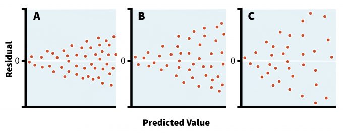
Parametric models assume that sampled populations have similar variances even if their means are different. This assumption becomes critical in studies comparing different groups of organisms, treatments, or sampling intervals and it is the responsibility of the researcher to make these considerations abundantly clear in the protocols of such studies. If the sample sizes are equal then parametric tests are fairly robust to the departure from homoscedasticity (i.e., equal variance of errors across the data) (Day and Quinn 1989, Sokal and Rohlf 1994). In fact, an equal sample size among different treatments or areas should be ensured whenever possible since most parametric tests are overly sensitive to violations of assumptions in situations with unequal sample sizes (Day and Quinn 1989). The best approach for detecting a violation in homoescedasticity, however, is plotting the residuals of the analysis against predicted values (i.e., residual analysis) (Crawley 2007). This plot can reveal the nature and severity of the potential disagreement/discord between variances (Figure 11.2), and is a standard feature in many statistical packages. Indeed, such visual inspection of the model residuals, in addition to the benefits outlined above, can help determine not only if there is a need for data transformation, but also the type of the distribution. Although several formal tests exist to determine the heterogeneity of variances (e.g., Bartlett’s test, Levine’s test), these techniques assume a normal data distribution, which reduces their utility in most ecological studies (Sokal and Rohlf 1994).
Normality
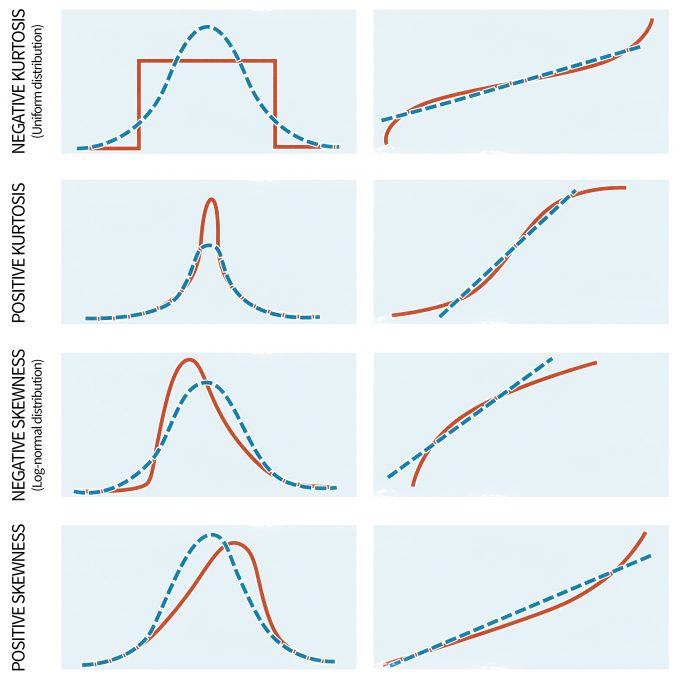
Although parametric statistics are fairly robust to violations of the assumption of normality, highly skewed distributions can significantly affect the results. Unfortunately, non-normality appears to be the norm in ecology; in other words ecological data only rarely follow a normal distribution (Potvin and Roff 1993, White and Bennetts 1996, Hayek and Buzas 1997, Zar 1999). Moreover, the normal distribution primarily describes continuous variables whereas count data, often the type of information gathered during monitoring programs, are discrete (Thompson et al. 1998, Krebs 1999). Thus, it is important to be vigilant for large departures from normality in your data. This can be done with a number of tests if your data meet certain specifications. For instance, if the sample size is equal among groups and sufficiently large (e.g., n > 20) you can implement tests to assess for normality or to determine the significance of non-normality. The latter is commonly done with several techniques, including the W-test and the Kolmogorov-Smirnov D-test for larger sample sizes. The applicability of both tests, however, is limited due to the fact that they exhibit a low power if the sample size is small and excessive sensitivity when the sample size is large. To overcome these complications, visual examinations of the data are also undertaken. Visual examinations are generally more appropriate than formal tests since they allow one to detect the extent and the type of problem. Keep in mind, however, that when working with linear models the aim is to “normalize” the data/residuals. Plotting the residuals with normal-probability plots (Figure 11.3), stem-and-leaf diagrams, or histograms can help to understand the nature of the non-normal data (Day and Quinn 1989).
Possible Remedies if Parametric Assumptions are Violated
Data transformations or non-parametric tests are often recommended as appropriate solutions if the data do not meet parametric assumptions (Sabin and Stafford 1990, Thompson et al. 1998). Those developing monitoring plans, however, should repeatedly (and loudly) advocate sound experimental design as the only effective prevention of many statistical problems. This will keep unorganized data collection and questionable data transformations to a minimum. There is no transformation or magical statistical button for data that are improperly collected. Nonetheless, a properly designed monitoring program is likewise not a panacea; ecosystems are complex. Thus even proper designs can produce data that confound analysis, are messy, and require some remedies if parametric models are to be used.
Data Transformation
If significant violations of parametric assumptions occur, it is customary to implement an appropriate data transformation to try to resolve the violations. During a transformation, data will be converted and analyzed at a different scale. In general, researchers should be aware of the need to back-transform the results after analysis to present parameter values on the original data scale or be clear that their results are being presented on a transformed scale. Examples of common types of transformations that a biometrician may recommend for use are presented in Table 11.2. A wisely chosen transformation can often improve homogeneity of variances and produce an approximation of a normal distribution.
| Transformation type | When appropriate to use |
| Logarithmic | Use with count data and when means positively correlate with variances. A rule of thumb suggests its use when the largest value of the response variable is at least 10 x the smallest value. |
| Square-root | Use with count data following a Poisson distribution. |
| Inverse | Use when data residuals exhibit a severe funnel shaped pattern, often the case in data sets with many near-zero values. |
| Arcsine square root | Good for proportional or binomial data. |
| Box-Cox objective approach | If it is difficult to decide on what transformation to use, this procedure finds an optimal model for the data. |
Nonparametric Alternatives
If the data violate basic parametric assumptions, and transformations fail to remedy the problem, then you may wish to use nonparametric methods (Sokal and Rohlf 1994, Thompson et al. 1998, Conover 1999). Nonparametric techniques have less stringent assumptions about the data, are less sensitive to the presence of outliers, and are often more intuitive and easier to compute (Hollander and Wolfe 1999). Since nonparametric models are less powerful than their parametric counterparts, however, parametric tests are preferred if the assumptions are met or data transformations are successful (Day and Quinn 1989, Johnson 1995).
Statistical Distribution of the Data
As mentioned above, plant and animal data are often in the form of counts of organisms and this can present special challenges during analyses. The probability that organisms occur in a particular habitat has a direct bearing on the selection of appropriate sampling protocols and statistical models (Southwood 1992). Monitoring data will most likely approximate random or clumped distributions, yet this should not be blindly assumed. Fitting the data to the Poisson or negative binomial models are common ways to test if they do (Southwood 1992, Zuur 2009). These models are also particularly appropriate for describing count data, which are, once again, examples of discrete variables (e.g., quadrat counts, sex ratios, ratios of juveniles to adults). The following subsections briefly describe how to identify whether or not the data follow either a Poisson or negative binomial distribution model.
Poisson Distribution
Poisson distributions are common among species, where the probability of detecting an individual in any sample is rather low (Southwood 1992). The Poisson model gives a good fit to data if the mean count (e.g., number of amphibians per sampling quadrat) is in the range of 1–5. As the mean number of individuals in the sample increases, and exceeds 10, however, the random distribution begins to approach the normal distribution (Krebs 1999, Zar 1999).
During sampling, the key assumption of the Poisson (random) distribution is that the expected number of organisms in a sample is the same and that it equals μ, the population mean (Krebs 1999, Zuur 2009). One intriguing property of the random distribution is that it can be described by its mean, and that the mean equals the variance (s2). The probability (frequency) of detecting a given number of individuals in a sample collected from a population with mean = μ is:
Pμ = e-μ(μμ/μ!)
Whether or not the data follow a random distribution can be tested with a simple Chi-square goodness of fit test or with an index of dispersion (I), which is expected to be 1.0 if the assumption of randomness is satisfied:
I = s2 / ̅x̅,
where ̅x̅ and s2 are the observed sample mean and variance, respectively.
Zurr et al. (2009) provided excellent examples of tests for goodness of fit for Poisson distributions. In practice, the presence of a Poisson distribution in data can also be assessed visually by examining the scatter pattern of residuals during analysis. If we reject the null hypothesis that samples came from a random distribution, s2 < μ, and s2/ μ < 1.0, then the sampled organisms are either distributed uniformly or regularly (underdispersed). If we reject the null hypothesis but the values of s2 and s2/ μ do not fall within those bounds, then the sampled organisms are clumped (overdispersed).
Negative Binomial Distribution
An alternative approach to the Poisson distribution, and one of the mathematical distributions that describe clumped or aggregated spatial patterns, is the negative binomial (Pascal) distribution (Anscombe 1973, Krebs 1999, Hilbe 2007, Zuur 2009). White and Bennetts (1996) suggested that this distribution is a better approximation to count data than the Poisson or normal distributions. The negative binomial distribution is described by the mean and the dispersion parameter k, which expresses the extent of clumping. As a result of aggregation, it always follows that s2 > μ and the index of dispersion (I) > 1.0. Several techniques exist to evaluate the goodness-of-fit of data to the negative binomial distribution. As an example, White and Bennetts (1996) give an example of fitting the negative binomial distribution to point-count data for orange-crowned warblers to compare their relative abundance among forest sites. Zero-inflated Poisson models (ZIP models) are recommended for analysis of count data with frequent zero values (e.g., rare species studies) or where data transformations are not feasible or appropriate (e.g., Heilbron 1994, Welsh et al. 1996, Hall and Berenhaut 2002, Zuur 2009). Good descriptions and examples of their use can be found in Krebs (1999), Southwood (1992), Faraway (2006), and Zurr et al. (2009). Since the variety of possible clumping patterns in nature is practically infinite, it is possible that the Poisson and negative binomial distributions may not always adequately fit the data at hand.
Analysis of Inventory Data – Abundance
Absolute Density or Population Size
National policy on threatened and endangered species is ultimately directed toward efforts to increase or maintain the total number of individuals of the species within their natural geographic range (Carroll et al. 1996). Total population size and effective population size (i.e., the number of breeding individuals in a population) (Harris and Allendorf 1989) are the two parameters that most directly indicate the degree of species endangerment and/or effectiveness of conservation policies and practices. Population density is informative for assessing population status and trends because the parameter is sensitive to changes in natural mortality, exploitation, and habitat quality. In some circumstances, it may be feasible to conduct a census of all individuals of a particular species in an area to determine the total population size or density parameters. Typically, however, population size and density parameters are estimated using statistical analyses based on only a sample of population members (Yoccoz et al. 2001, Pollock et al. 2002). Population densities of plants and sessile animals can be estimated from counts taken on plots or data describing the spacing between individuals (i.e., distance methods) and are relatively straightforward. Population analyses for many animal species must account for animal response to capture or observation, observer biases, and different detection probabilities among sub-populations (Kery and Schmid 2004). For instance, hiring multiple technicians for field-work and monitoring a species whose behavior or preferred habitat change seasonally are two factors that would need to be addressed in the analysis. Pilot studies are usually required to collect the data necessary to do this. Furthermore, the more common techniques used for animal species, such as mark-recapture studies, catch-per-unit effort monitoring programs, and occupancy studies, require repeated visits to sampling units. This, along with the need for pilot studies, increases the complexity and cost of monitoring to estimate population parameters relative to monitoring of sessile organisms.
For animal species, mark-recapture models are often worth the extra investment in terms of the data generated as they may be used to estimate absolute densities of populations and provide additional information on such vital statistics as animal movement, geographic distribution, and survivorship (Lebreton et al. 1992, Nichols 1992, Nichols and Kendall 1995, Thomson et al. 2009). Open mark-recapture models (e.g., Jolly-Seber) assume natural changes in the population size of the species of interest during sampling. In contrast, closed models assume a constant population size. Program MARK (White et al. 2006) performs sophisticated maximum-likelihood-based mark-recapture analyses and can test and account for many of the assumptions such as open populations and heterogeneity.
Relative Abundance Indices
It is sometimes the case that data analyses for biological inventories and monitoring studies can be accomplished based on indices of population density or abundance, rather than population estimators (Pollock et al. 2002). The difference between estimators and indices is that the former yield absolute values of population density while the latter provide relative measures of density that can be used to assess population differences in space or time. Caughley (1977) advocated the use of indices after determining that many studies that used estimates of absolute density could have used density indices without losing information. He suggested that use of indices often results in much more efficient use of time and resources and produces results with higher precision (Caughley 1977, Caughley and Sinclair 1994). Engeman (2003) also indicated that use of an index may be the most efficient means to address population monitoring objectives and that the concerns associated with use of indices may be addressed with appropriate and thorough experimental design and data analyses. It is important, therefore, to understand these concerns before utilizing an index, even though indices of relative abundance have a wide support among practitioners who often point out their efficiency and higher precision (Caughley 1977, Engeman 2003). First, they are founded on the assumption that index values are closely associated with values of a population parameter. Because the precise relationship between the index and parameter usually is not quantified, the reliability of this assumption is often brought into question (Thompson et al. 1998, Anderson 2001). Also, the opportunity for bias associated with indices of abundance is quite high. For instance, track counts could be related to animal abundance, animal activity levels, or both. Indices often are used because of logistical constraints. Capture rates of animals over space and time may be related to animal abundance or to their vulnerability to capture in areas of differing habitat quality. If either of these techniques are used to generate the index, considerable caution must be exercised when interpreting results. Given these concerns, the utility of a pilot study that will allow determination, with a known level of certainty, of the relationship between the index and the actual population (or fitness) for the species being monitored is clear. Determining this relationship, however, requires an estimate of the population.
Suitability of any technique, including indices, should ultimately be based on how well it addresses the study objective and the reliability of its results (Thompson 2002). It is also important to consider that statistical analyses of relative abundance data require familiarity with the basic assumptions of parametric and non-parametric models. Some examples of the use and analysis of relative density data can be found in James et al. (1996), Rotella et al. (1996), Knapp and Matthews (2000), Huff et al. (2000), and Rosenstock et al. (2002).
Analyses of relative abundance data require familiarity with the basic assumptions of parametric models. Since the focus is on count data, alternative statistical methods can be employed to fit the distribution of the data (e.g., Poisson or negative binomial). Although absolute abundance techniques are independent of parametric assumptions, they nevertheless do have their own stringent requirements.
When a researcher decides to use a monitoring index, it is important to remember that statistical power negatively correlates with the variability of the monitoring index. This truly underscores the need to choose an appropriate indicator of abundance and accurately estimate its confidence interval (Harris 1986, Gerrodette 1987, Gibbs et al. 1999). An excellent overview of a variety of groups of animals and plants for which the variability in estimating their population is known is given in Gibbs et al. (1998). It is also important to keep in mind that relative measures of density can be less robust to changes in habitat than absolute measures. For instance, forest practices may significantly affect indices that rely on visual observations of organisms. Although these factors may confound absolute measures as well, modern distance and mark-recapture analysis methods can account for variations in sightability and trapability. See Caughley (1977), Thompson et al. (1998), Rosenstock et al. (2002), Pollock et al. (2002) and Yoccoz et al. (2001) for in-depth discussions of the merits and limitations of estimating relative vs. absolute density in population monitoring studies.
Generalized Linear Models and Mixed Effects
Recently, generalized linear models (GLM) have become increasingly popular and take advantage of the data’s true distribution without trying to normalize it (Faraway 2006, Bolker 2008, McCulloch et al. 2008). Often times, the standard linear model cannot handle non-normal responses, such as counts or proportions, whereas generalized linear models were developed to handle categorical, binary, and other response types (Faraway 2006, McCulloch et al. 2008). In practice, most data have non-normal errors, and so GLMs allow the user to specify a variety of error distributions. This can be particularly useful with count data (e.g., Poisson errors), binary data (e.g., binomial errors), proportion data (e.g., binomial errors), data showing a constant coefficient of variation (e.g., gamma errors), and survival analysis (e.g., exponential errors) (Crawley 2007).
An extension of the GLM is the Generalized Linear Mixed Model (GLMM) approach. GLMMs are examples of hierarchal models and are most appropriate when dealing with nested data. What are nested data? As an example, monitoring programs may collect data on species abundances or occurrences from multiple sites on different sampling occasions within each site. Alternatively, researchers might also sample from a single site in different years. In both cases, the data are “nested” within a site or a year, and to analyze the data generated from these surveys without considering the “site” or “year” effect would be considered pseudoreplication (Hurlbert 1984). That is, there is a false assumption of independency of the sampling occasions within a single site or across the sampling period. Traditionally, researchers might avoid this problem by averaging the results of those sampling occasions across the sites or years and focus on the means, or they may simply just focus their analysis within an individual site or sampling period. The more standard statistical approaches, however, attempt to quantify the exact effect of the predictor variables (e.g., forest area, forb density), but ecological problems often involve random effects that are a result of the variation among sites or sampling periods (Bolker et al. 2009). Random effects that come from the same group (e.g., site or time period) will often be correlated, thus violating the standard assumption of independence of errors in most statistical models.
Hierarchal models offer an excellent way of dealing with these problems, but when using GLMMs, researchers should be able to correctly identify the difference between a fixed effect and a random effect. In its most basic form, fixed effects have “informative” factor levels, while random effects often have “uninformative” factor levels (Crawley 2007). That is, random effects have factor levels that can be considered random samples from a larger population (e.g., blocks, sites, years). In this case, it is more appropriate to model the added variation caused by the differences between the levels of the random effects and the variation in the response variables (as opposed to differences in the mean). In most applied situations, random effect variables often include site names or years. In other cases, when multiple responses are measured on an individual (e.g., survival), random effects can include individuals, genotypes, or species. In contrast, fixed effects then only model differences in the mean of the response variable, as opposed to the variance of the response variable across the levels of the random effect, and can include predictor environmental variables that are measured at a site or within a year. In practice, these distinctions are at times difficult to make and mixed effects models can be challenging to apply. For example, in his review of 537 ecological studies that used GLMM analyses, Bolker (2009) found that 58% used this tool inappropriately. Consequently, as is the case with many of these procedures, it is important to consult with a statistician when developing and implementing your analysis. There several excellent reviews and books on the subject of mixed effects modeling (Gelman and Hill 2007, Bolker et al. 2009, Zuur 2009).
Analysis of Species Occurrences and Distribution
Does a species occur or not occur with reasonable certainty in an area under consideration for management? Where is the species likely to occur? These types of questions have been and continue to be of interest for many monitoring programs (MacKenzie 2005, MacKenzie 2006). Data on species occurrences are often more cost-effective to collect than data on species abundances or demographic data. Traditionally, information on species occurrences has been used to:
- Identify habitats that support the lowest or highest number of species,
- Shed light on the species distribution, and
- Point out relationships between habitat attributes (e.g., vegetation types, habitat structural features) and species occurrence or community species richness.
For many monitoring programs, species occurrence data are often considered preliminary data only collected during the initial phase of an inventory project and often to gather background information for the project area. In recent years, however, occupancy modeling and estimation (MacKenzie et al. 2002, MacKenzie et al. 2005, Mackenzie and Royle 2005, MacKenzie 2006) has become a critical aspect of monitoring animal and plant populations. These types of categorical data have represented an important source of data for many monitoring programs that have targeted rare or elusive species, or where resources are unavailable to collect data required for parameter estimation models (see Hayek and Buzas 1997, Thompson 2004).
For some population studies, simply determining whether a species is present in an area may be sufficient for conducting the planned data analysis. For example, biologists attempting to conserve a threatened wetland orchid may need to monitor the extent of the species range and proportion of occupied area (POA) on a National Forest. One hypothetical approach is to map all wetlands in which the orchid is known to be present, as well as additional wetlands that may qualify as the habitat type for the species within the Forest. To monitor changes in orchid distribution at a coarse scale, data collection could consist of a semiannual monitoring program conducted along transects at each of the mapped wetlands to determine if at least one individual orchid (or some alternative criterion to establish occupancy) is present. Using only a list that includes the wetland label (i.e., the unique identifier), the monitoring year, and an occupancy indicator variable, the biologists could prepare a time series of maps displaying all of the wetlands by monitoring year and distinguish the subset of wetlands that were found to be occupied by the orchid.
Monitoring programs to determine the presence of a species typically require less sampling intensity than fieldwork necessary to collect other population statistics. It is far easier to determine if there is at least one individual of the target species on a sampling unit than it is to count all of the individuals. Conversely, to determine with confidence that a species is not present on a sampling unit requires more intensive sampling than collecting count or frequency data because it is so difficult to dismiss the possibility that an individual missed detection (i.e., a failure to detect does not necessarily equate to absence). Traditionally, the use of occurrence data was considered a qualitative assessment of changes in the species distribution pattern and served as an important first step to formulating new hypotheses as to the cause of the observed changes. More recently, however, repeated sampling and the use occupancy modeling estimation has increased the applicability of occurrence data in ecological monitoring.
Possible analysis models for occurrence data
Species diversity
The number of species per sample (e.g., 1-m2 quadrat) can give a simple assessment of local, α diversity, or these data may be used to compare species composition among several locations (β diversity) using simple binary formulas such as the Jaccard’s index or Sorensen coefficient (Magurran 1988). For example, the Sorensen qualitative index may be calculated as:
CS = 2j / (a +b),
where a and b are numbers of species in locations A and B, respectively, and j is the number of species found at both locations. If species abundance is known (number individuals/species), species diversity can be analyzed with a greater variety of descriptors such as numerical species richness (e.g., number species/number individuals), quantitative similarity indices (e.g., Sorensen quantitative index, Morista-Horn index), proportional abundance indices (e.g., Shannon index, Brillouin index), or species abundance models (Magurran 1988, Hayek and Buzas 1997).
Binary Analyses
Since detected/not-detected data are categorical, the relationship between species occurrence and explanatory variables can be modeled with a logistic regression if values of either 1 (species detected) or 0 (species not-detected) are ascribed to the data (Trexler and Travis 1993, Hosmer and Lemeshow 2000, Agresti 2002). Logistic regression necessitates a dichotomous (0 or 1) or a proportional (ranging from 0 to 1) response variable. Yet in many cases, logistic regression is used in combination with a set of variables to predict the detection or non-detection a species. For example, a logistic regression can be enriched with such predictors as the percentage of vegetation cover, forest patch area, or presence of snags to create a more informative model of the occurrence of a forest-dwelling bird species. The resulting logistic function provides an index of probability with respect to species occurrence. There are a number of cross-validation functions that allow the user to identify the probability value that best separates sites where a species was found from where it was not found based on the existing data (Freeman and Moisen 2008). In some cases, data points are withheld from formal analysis (e.g., validation data) and used to test the relationships after the predictive relationships are developed using the rest of data (e.g., training data) (Harrell 2001). Logistic regression, however, is a parametric test. If the data do not meet or approximate the parametric assumption, alternatives to standard logistic regression can be used including General Additive Models (GAM) and variations of classification tree (CART) analyses.
Prediction of species density
In some cases, occurrence data have been used to predict organism density if the relationship between species occurrence and density is known and the model’s predictive power is reasonably high (Hayek and Buzas 1997). For example, one can record plant abundance and species richness in sampling quadrats. The species proportional abundance, or constancy of its frequency of occurrence (Po), can then be calculated as:
Po = No. of species occurrences (+ or 0) / number of samples (quadrats)
Consequently, the average species density is plotted against its proportional abundance to derive a model to predict species abundance in other locations with only occurrence data. Note, however, that the model may function reasonably well only in similar and geographically related types of plant communities (Hayek and Buzas 1997).
Occupancy Modeling
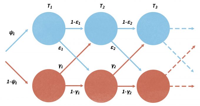
Note that without a proper design, detected/not-detected data cannot be reliably used to measure or describe species distributions (Kery and Schmid 2004, MacKenzie 2006, Kéry et al. 2008). Although traditional methods using logistic regression and other techniques may be used to develop a biologically-based model that can predict the probability of occurrence of a site over a landscape, occupancy modeling has developed rapidly over the past few years. As with mark-recapture analysis, changes in occupancy over time can be parameterized in terms of local extinction (ε) and colonization (γ) processes, analogous to the population demographic processes of mortality and recruitment (Figure 11.4) (MacKenzie et al. 2003, MacKenzie 2006, Royle and Dorazio 2008). In this case, sampling must be done in a repeated fashion within separate primary sampling periods (Figure 11.4). Occupancy models are robust to missing observations and can effectively model the variation in detection probabilities between species. Of greatest importance, occupancy (ψ), colonization (γ), and local extinction (ε) probabilities can be modeled as functions of environmental covariate variables that can be site-specific, count-specific, or change between the primary periods (MacKenzie et al. 2003, MacKenzie et al. 2009). In addition, detection probabilities can also be functions of season-specific covariates and may change with each survey of a site. More recently, program PRESENCE has been made available as a sophisticated likelihood-based family of models that has been increasingly popular using species occurrence in for monitoring (www.mbr-pwrc.usgs.gov/software/presence.html). Donovan and Hines (2007) also present an explanation of occupancy models and several online exercises (www.uvm.edu/envnr/vtcfwru/spreadsheets/occupancy/occupancy.htm).
Assumptions, data interpretation, and limitations
It is crucial to remember that failure to detect a species in a habitat does not mean that the species was truly absent (Kery and Schmid 2004, MacKenzie 2006, Kéry et al. 2008). Cryptic or rare species, such as amphibians, are especially prone to under-detection and false absences (Thompson 2004). Keep in mind that occasional confirmations of species presence provide only limited data. For example, the use of a habitat by a predator may reflect prey availability, which may fluctuate annually or even during one year. A more systematic approach with repeated visits is necessary to generate more meaningful data (Mackenzie and Royle 2005).
Extrapolating density without understanding the species requirements is also likely to produce meaningless results since organisms depend on many factors that we typically do not understand. Furthermore, limitations of species diversity measures should be recognized, especially in conservation projects. For example, replacement of a rare or keystone species by a common or exotic species would not affect species richness of the community and could actually ‘improve’ diversity metrics. Also, the informative value of qualitative indices is rather low since they disregard species abundance and are sensitive to differences in sample size (Magurran 1988). Rare and common species are weighted equally in community comparisons. Often this may be an erroneous assumption since the effect of a species on the community is expected to be proportional to its abundance; keystone species are rare exceptions (Power and Mills 1995). In addition, analyses that focus on species co-occurrences without effectively modeling or taking into account the varying detection probabilities of the species can be prone to error, although new occupancy models are beginning to incorporate detectability in models of species richness (MacKenzie et al. 2004, Royle et al. 2007, Kéry et al. 2009).
Analysis of Trend Data
Trend models should be used if the objective of a monitoring plan is to detect a change in a population parameter over time. Most commonly, population size is repeatedly estimated at set time intervals. Trend monitoring is crucial in the management of species since it may help:
- Recognize population decline and focus attention on affected species,
- Identify environmental variables correlated with the observed trend and thus help formulate hypotheses for cause-and-effect studies, and
- Evaluate the effectiveness of management decisions (Thomas 1996, Thomas and Martin 1996).
The status of a population can be assessed by comparing observed estimates of the population size at some time interval against management-relevant threshold values (Gibbs et al. 1999, Elzinga et al. 2001). All monitoring plans, but particularly those designed to generate trend data, should emphasize that the selection of reliable indicators or estimators of population change is a key requirement of effective monitoring efforts. Indices of relative abundance are often used in lieu of measures of actual population size, sometimes because of the relatively reduced cost and effort needed to collect the necessary data on an iterative basis. For example, counts of frog egg masses may be performed annually in ponds (Gibbs et al. 1998) or bird point-counts may be taken along sampling routes (Böhning-Gaese et al. 1993, Link and Sauer 1997a,b; 2007). Analysis of distribution maps, checklists, and volunteer-collected data may also provide estimates of population trends (Robbins 1990, Temple and Cary 1990, Cunningham and Olsen 2009, Zuckerberg et al. 2009). To minimize the bias in detecting a trend, such as in studies of sensitive species, the same population may be monitored using different methods (e.g., a series of different indices) (Temple and Cary 1990). Data may also be screened prior to analysis. For example, only monitoring programs that meet agreed-upon criteria may be included, or species with too few observations may be excluded from the analysis (Thomas 1996, Thomas and Martin 1996).
Possible Analysis Models
Trends over space and time present many challenges for analysis to the extent that consensus does not exist on the most appropriate method to analyze the related data. This is a significant constraint since model selection may have a considerable impact on interpretation of the results of analysis (Thomas 1996, Thomas and Martin 1996).
Poisson regression is independent of parametric assumptions and is especially appropriate for count data. Classic linear regression models in which estimates of population size are plotted against biologically relevant sampling periods have been historically used in population studies since they are easy to calculate and interpret. However, these models are subject to parametric assumptions, which are often violated in count data (Krebs 1999, Zar 1999). Linear regressions also assume a constant linear trend in data, and expect independent and equally spaced data points. Since individual measurements in trend data are autocorrelated, classic regression can give skewed estimates of standard errors and confidence intervals, and inflate the coefficient of determination (Edwards and Coull 1987, Gerrodette 1987). Edwards and Coull (1987) suggested that correct errors in linear regression analysis can be modeled using an autoregressive process model (ARIMA model). Linear route-regression models represent a more robust form of linear regression and are popular with bird ecologists in analyses of roadside monitoring programs (Geissler and Sauer 1990, Sauer et al. 1996, Thomas 1996). They can handle unbalanced data by performing analysis on weighted averages of trends from individual routes (Geissler and Sauer 1990) but may be sensitive to nonlinear trends (Thomas 1996). Harmonic or periodic regressions do not require regularly spaced data points and are valuable in analyzing data on organisms that display significant daily periodic trends in abundance or activity (Lorda and Saila 1986).
For some data where large sample sizes are not possible, or where variance structure cannot be estimated reliably, alternative analytical approaches may be necessary. This is especially true when the risk of concluding that a trend cannot be detected is caused by large variance or small sample sizes, the species is rare, and the failure to detect a trend could be catastrophic for the species. Wade (2000) provides an excellent overview of the use of Bayesian analysis to address these types of problems. Thomas (1996) gives a thorough review of the most popular models fit to trend data and assumptions associated with their use.
Assumptions, Data Interpretation, and Limitations
The underlying assumption of trend monitoring projects is that a population parameter is measured at the same sampling points (e.g., quadrats, routes) using identical or similar procedures (e.g., equipment, observers, time period) at regularly spaced intervals. If these requirements are violated, data may contain excessive noise, which may complicate their interpretation. Thomas (1996) identified four sources of variation in trend data:
- Prevailing trend – population tendency of interest (e.g., population decline),
- Irregular disturbances – disruptions from stochastic events (e.g., drought mortality),
- Partial autocorrelation – dependence of the current state of the population on its previous levels, and
- Measurement error – added data noise from deficient sampling procedures.
Although trend analyses are useful in identifying population change, the results are correlative and tell us little about the underlying mechanisms. Ultimately, only well designed cause-and-effect studies can validate causation and facilitate management decisions.
Analysis of Cause and Effect Monitoring Data
The strength of trend studies lies in their capacity to detect changes in population size. To understand the reason for population fluctuations, however, the causal mechanism behind the population change must be determined. Cause-and-effect studies represent one of the strongest approaches to test cause-and-effect relationships and are often used to assess effects of management decisions on populations. Similar to trend analyses, cause-and-effect analyses may be performed on indices of relative abundance or absolute abundance data.
Possible analysis models
Parametric and distribution free (non-parametric) models provide countless alternatives to fitting cause-and-effect data (Sokal and Rohlf 1994, Zar 1999). Excellent introductory material to the design and analysis of ecological experiments, specifically for ANOVA models, can be found in Underwood (1997) and Scheiner and Gurevitch (2001).
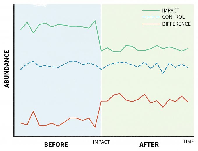
A unique design is recommended for situations where a disturbance (treatment) is applied and its effects are assessed by taking a series of measurements before and after the perturbation (Before-After Control-Impact, BACI) (Stewart-Oaten et al. 1986) (Figure 11.5). This model was originally developed to study pollution effects (Green 1979), but it has found suitable applications in other areas of ecology as well (Wardell-Johnson and Williams 2000, Schratzberger et al. 2002, Stanley and Knopf 2002). In its original design, an impact site would have a parallel control site. Further, variables deemed at the beginning of the study to be relevant to the management actions would be planned to be periodically monitored over time. Then any differences between the trends of those measured variables in the impact site with those from the control site (treatment effect) would be demonstrated as a significant time*location interaction (Green 1979). This approach has been criticized since the design was originally limited to unreplicated impact and control sites (Figure 11.5), but it can be improved by replicating and randomly assigning sites (Hurlbert 1984, Underwood 1994).
Assumptions, data interpretation, and limitations
Since cause-and-effect data are frequently analyzed with ANOVA models, a parametric model, one must pay attention to parametric assumptions. Alternative means of assessing manipulative studies may also be employed. For example, biologically significant effect size with confidence intervals may be used in lieu of classic statistical hypothesis testing. An excellent overview of arguments in support of this approach with examples may be found in Hayes and Steidl (1997)), Steidl et al. (1997), Johnson (1999), and Steidl and Thomas (2001).
Paradigms of Inference: Saying Something With Your Data and Models
Randomization tests
These tests are not alternatives to parametric tests, but rather are unique means of estimating statistical significance. They are extremely versatile and can be used to estimate test statistics for a wide range of models, and are especially valuable in analyzing non-randomly selected data points. It is important to keep in mind, however, that randomization tests are computationally difficult even with small sample sizes (Edgington and Onghena 2007). A statistician needs to be involved in choosing to use and implement these techniques. More information on randomization tests and other computation-intensive techniques can be found in Crowley (1992), Potvin and Roff (1993), and Petraitis et al. (2001).
Information Theoretic Approaches: Akaike’s Information Criterion
Akaike’s information criterion (AIC), derived from information theory, may be used to select the best-fitting model among a number of a priori alternatives. This approach is more robust and less arbitrary than hypothesis-testing methods since the P-value is often predominantly a function of sample size. AIC can be easily calculated for any maximum-likelihood based statistical model, including linear regression, ANOVA, and general linear models. The model hypothesis with the lowest AIC value is generally identified as the ’best‘ model with the greatest support (given the data) (Burnham and Anderson 2002). Once the best model has been identified, the results can then be interpreted based on the changes in the explanatory variables over time. For instance, if the amount of mature forest near streams were associated with the probability of occurrence of tailed frogs, then a map generated over the scope of inference could be used to identify current and likely future areas where tailed frogs could be vulnerable to management actions. In addition, one of the more useful advantages of using information theoretic approaches is that identifying a single, best model is not necessary. Using the AIC metric (or any other information criteria), one can rank models and can average across models to calculate weighted parameter estimates or predictions (i.e., model averaging). A more in depth discussion of practical uses of AIC may be found in Burnham and Anderson (2002) and Anderson (2008).
Bayesian Inference
Bayesian statistics refers to a distinct approach to making inference in the face of uncertainty. In general, Bayesian statistics share much with the traditional frequentist statistics with which most ecologists are familiar. In particular, there is a similar reliance on likelihood models which are routinely applied by most statisticians and biometricians. Bayesian inference can also be used in a variety of statistical tasks, including parameter estimation and hypothesis testing, post hoc multiple comparison tests, trend analysis, ANOVA, and sensitivity analysis (Ellison 1996). Bayesian methods, however, test hypotheses not by rejecting or accepting them, but by calculating their probabilities of being true. Thus, P-values, significance levels and confidence intervals are moot points (Dennis 1996). Based on existing knowledge, investigators assign a priori probabilities to alternative hypotheses and then use data to calculate (“verify”) posterior probabilities of the hypotheses with a likelihood function (Bayes theorem). The highest probability identifies the hypothesis that is the most likely to be true given the experimental data (Dennis 1996, Ellison 1996). Bayesian statistics has several key features that differ from classical frequentist statistics:
- Bayes is based on an explicit mathematical mechanism for updating and propagating uncertainty (Bayes theorem)
- Bayesian analyses quantify inferences in a simpler, more intuitive manner. This is especially true in management settings that require making decisions under uncertainty
- Takes advantage of pre-existing data, and may be used with small sample sizes
For example, conclusions of a monitoring analysis could be framed as: “There is a 65% chance that clearcutting will negatively affect this species,” or “The probability that this population is declining at a rate of 3% per year is 85%.” A more in-depth coverage of the use of Bayesian inference in ecology can be found in Dennis (1996), Ellison (1996), Taylor et al. (1996), Wade (2000), and O’Hara et al. (2002). Even though Bayesian inference is easy to grasp and perform, it is still relatively rare in natural resources applications (although that is quickly changing) and sufficient support resources for these types of tests may not be readily available. It is recommended that it only be implemented with the assistance of a consulting statistician.
Retrospective Power Analysis
Does the outcome of a statistical test suggest that no real biological change took place at the study site? Did the change actually occur but was not detected due to a low power of the statistical test used, in other words, was a Type II (missed-change) error committed in the process? It is recommended that those undertaking inventory studies should routinely evaluate the validity of results of statistical tests by performing a post hoc, or retrospective power analysis for two important reasons:
- The possibility of falsely accepting the null hypothesis is quite real in ecological studies, and
- A priori calculations of statistical power are only rarely performed in practice, but are critical to data interpretation and extrapolation (Fowler 1990).
A power analysis is imperative whenever a statistical test turns out to be non-significant and fails to reject the null hypothesis (H0); for example, if P > 0.05 at 95% significance level. There are a number of techniques to carry out a retrospective power analysis well. For instance, they should be performed only using an effect size other than the effect size observed in the study (Hayes and Steidl 1997, Steidl et al. 1997). In other words, post hoc power analyses can only answer whether or not the performed study in its original design would have allowed detecting the newly selected effect size.
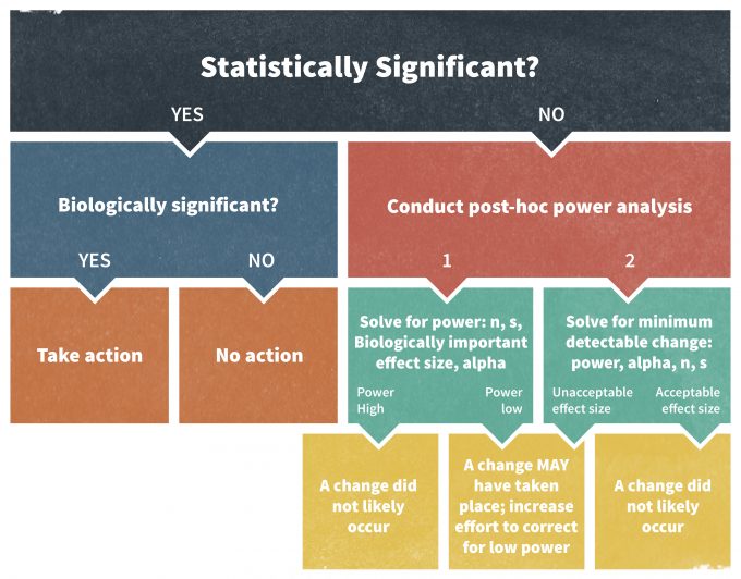
Elzinga et al. (2001) recommends the following approach to conducting a post hoc power analysis assessment (Figure 11.6). If a statistical test was declared non-significant, one could calculate a power value to detect a biologically significant effect of interest, usually a trigger point tied to a management action. If the resulting power is low, one must take precautionary measures in the monitoring program. Alternatively, one can calculate a minimum detectable effect size at a selected power level. An acceptable power level in wildlife studies is often set at about 0.80 (Hayes and Steidl 1997). If the selected power can only detect a change that is larger than the trigger point value, the outcome of the study should again be viewed with caution.
Monitoring plans may also encourage the use of confidence intervals as an alternative approach to performing a post hoc power analysis. This method is actually superior to power analysis since confidence intervals not only suggest whether or not the effect was different from zero, but they also provide an estimate of the likely magnitude of the true effect size and its biological significance. Ultimately, for scientific endeavors these are rules of thumb. In management contexts, however, decision making under uncertainty where the outcomes have costs, power calculations and other estimates for acceptable amounts of uncertainty should be approached more rigorously.
Summary
Even before the collection of data, researchers must consider which analytical techniques will likely be appropriate to interpret their data. Techniques will be highly dependent on the design of the monitoring program, so a monitoring plan should clearly articulate the expected analytical approaches after consulting with a biometrician. After data collection but before statistical analyses are conducted, it is often helpful to view the data graphically to understand data structure. Assumptions upon which certain techniques are based (e.g., normality, independence of observations and uniformity of variances for parametric analyses) should be tested. Some violations of assumptions may be addressed with transformations, while others may need different approaches. Detected/non-detected, count data, time series and before-after control impact designs all have different data structures and will need to be analyzed in quite different ways. Given the considerable room for spurious analysis and subsequent erroneous interpretation, if possible, a biometrician/statistician should be consulted throughout the entire process of data analysis.
References
Agresti, A. 2002. Categorical data analysis. 2nd edition. John Wiley & Sons, New York, New York.
Anderson, D.R. 2001. The need to get the basics right in wildlife field studies. Wildlife Society Bulletin 29:1294-1297.
Anderson, D.R. 2008. Model based inference in the life sciences: a primer on evidence. Springer, New York, New York.
Anderson, D.R., K.P. Burnham, W.R. Gould, and S. Cherry. 2001. Concerns about finding effects that are actually spurious. Widlife Society Bulletin 29:311-316.
Anscombe, F.J. 1973. Graphs in statistical-analysis. American Statistician 27:17-21.
Böhning-Gaese, K., M.L. Taper, and J.H. Brown. 1993. Are declines in North American insectivorous songbirds due to causes on the breeding range. Conservation Biology 7:76-86.
Bolker, B.M. 2008. Ecological models and data in R. Princeton University Press, Princeton, New Jersey. 408pp.
Bolker, B.M., M.E. Brooks, C.J. Clark, S.W. Geange, J.R. Poulsen, M.H.H. Stevens, and J.S.S. White. 2009. Generalized linear mixed models: a practical guide for ecology and evolution. Trends in Ecology & Evolution 24:127-135.
Burnham, K.P., and D.R. Anderson. 2002. Model selection and inference: a practical information-theoretic approach. Springer-Verlag, New York, New York, USA. 454pp.
Carroll, R., C. Augspurger, A. Dobson, J. Franklin, G. Orians, W. Reid, R. Tracy, D. Wilcove, and J. Wilson. 1996. Strengthening the use of science in achieving the goals of the endangered species act: An assessment by the Ecological Society of America. Ecological Applications 6:1-11.
Caughley, G. 1977. Analysis of vertebrate populations. John Wiley & Sons, New York, New York.
Caughley, G., and A. R. E. Sinclair. 1994. Wildlife management and ecology. Blackwell Publishing, Malden, MA.
Cleveland, W.S. 1985. The elements of graphing data. Wadsworth Advanced Books and Software, Monterey, Calif.
Cochran, W.G. 1977. Sampling techniques. 3rd edition. John Wiley & Sons, New York.
Conover, W.J. 1999. Practical nonparametric statistics. 3rd edition. Wiley, New York.
Crawley, M.J. 2005. Statistics: an introduction using R. John Wiley & Sons, Ltd, West Sussex, England.
Crawley, M.J. 2007. The R Book. John Wiley & Sons, Ltd, West Sussex, England.
Crowley, P.H. 1992. Resampling methods for computation-intensive data-analysis in ecology and evolution. Annual Review of Ecology and Systematics 23:405-447.
Cunningham, R.B., and P. Olsen. 2009. A statistical methodology for tracking long-term change in reporting rates of birds from volunteer-collected presence-absence data. Biodiversity and Conservation 18:1305-1327.
Day, R.W., and G.P. Quinn. 1989. Comparisons of treatments after an analysis of variance in ecology. Ecological Monographs 59:433-463.
Dennis, B. 1996. Discussion: Should ecologists become Bayesians? Ecological Applications 6:1095-1103.
Donovan, T.M., and J. Hines. 2007. Exercises in occupancy modeling and estimation. www.uvm.edu/envnr/vtcfwru/spreadsheets/occupancy/occupancy.htm
Edgington, E.S., and P. Onghena. 2007. Randomization tests. 4th edition. Chapman & Hall/CRC, Boca Raton, FL.
Edwards, D., and B.C. Coull. 1987. Autoregressive trend analysis – an example using long-term ecological data. Oikos 50:95-102.
Ellison, A.M. 1996. An introduction to Bayesian inference for ecological research and environmental decision-making. Ecological Applications 6:1036-1046.
Elzinga, C.L., D.W. Salzer, and J.W. Willoughby. 1998. Measuring and monitoring plant plant populations. Technical Reference 1730-1., Bureau of Land Management, National Business Center, Denver, CO.
Elzinga, C.L., D.W. Salzer, J.W. Willoughby, and J.P. Gibbs. 2001. Monitoring plant and animal populations. Blackwell Science, Inc., Malden, Massachusetts.
Engeman, R.M. 2003. More on the need to get the basics right: population indices. Wildlife Society Bulletin 31:286-287.
Faraway, J. J. 2006. Extending the linear model with R: generalized linear, mixed effects and nonparametric regression models. Chapman & Hall/CRC, Boca Raton.
Fortin, M.-J., and M.R.T. Dale. 2005. Spatial analysis : a guide for ecologists. Cambridge University Press, Cambridge, UK ; New York.
Fowler, N. 1990. The 10 most common statistical errors. Bulletin of the Ecological Society of America 71:161-164.
Freeman, E.A., and G.G. Moisen. 2008. A comparison of the performance of threshold criteria for binary classification in terms of predicted prevalence and kappa. Ecological Modelling 217:48-58.
Geissler, P.H., and J.R. Sauer. 1990. Topics in route-regression analysis. Pages 54-57 in J.R. Sauer and S.Droege, editors. Survey designs and statistical methods for the estimation of avian population trends. USDI Fish and Wildlife Service, Washington, DC.
Gelman, A., and J. Hill. 2007. Data analysis using regression and multilevel/hierarchical models. Cambridge University Press, Cambridge ; New York.
Gerrodette, T. 1987. A power analysis for detecting trends. Ecology 68:1364-1372.
Gibbs, J.P., S. Droege, and P. Eagle. 1998. Monitoring populations of plants and animals. Bioscience 48:935-940.
Gibbs, J.P., H.L. Snell, and C.E. Causton. 1999. Effective monitoring for adaptive wildlife management: Lessons from the Galapagos Islands. Journal of Wildlife Management 63:1055-1065.
Gotelli, N.J., and A.M. Ellison. 2004. A Primer of Ecological Statistics. Sinaeur, Sunderland, MA.
Green, R.H. 1979. Sampling design and statistical methods for environmental biologists. Wiley, New York.
Gurevitch, J., J.A. Morrison, and L.V. Hedges. 2000. The interaction between competition and predation: A meta-analysis of field experiments. American Naturalist 155:435-453.
Hall, D.B., and K.S. Berenhaut. 2002. Score test for heterogeneity and overdispersion in zero-inflated Poisson and Binomial regression models. The Canadian Journal of Statistics 30:1-16.
Harrell, F.E. 2001. Regression modeling strategies with applications to linear models, logistic regression, and survival analysis. Springer, New York.
Harris, R.B. 1986. Reliability of trend lines obtained from variable counts. Journal of Wildlife Management 50:165-171.
Harris, R.B., and F.W. Allendorf. 1989. Genetically effective population size of large mammals – an assessment of estimators. Conservation Biology 3:181-191.
Hayek, L.-A.C., and M.A. Buzas. 1997. Surveying natural populations. Columbia University Press, New York.
Hayes, J.P., and R.J. Steidl. 1997. Statistical power analysis and amphibian population trends. Conservation Biology 11:273-275.
Hedges, L.V., and I. Olkin. 1985. Statistical methods for meta-analysis. Academic Press, Orlando.
Heilbron, D. 1994. Zero-altered and other regression models for count data with added zeros. Biometrical Journal 36:531-547.
Hilbe, J. 2007. Negative binomial regression. Cambridge University Press, Cambridge ; New York.
Hilborn, R., and M. Mangel. 1997. The ecological detective: confronting models with data. Princeton University Press, Princeton, NJ.
Hollander, M., and D.A. Wolfe. 1999. Nonparametric statistical methods. 2nd edition. Wiley, New York.
Hosmer, D.W., and S. Lemeshow. 2000. Applied logistic regression. 2nd edition. Wiley, New York.
Huff, M.H., K.A. Bettinger, H.L. Ferguson, M.J. Brown, and B. Altman. 2000. A habitat-based point-count protocol for terrestrial birds, emphasizing Washington and Oregon. USDA Forst Service General Technical Report, PNW-GTR-501.
Hurlbert, S.H. 1984. Pseudoreplication and the design of ecological field experiments. Ecological Monographs 54:187-211.
James, F.C., C.E. McCullogh, and D.A. Wiedenfeld. 1996. New approaches to the analysis of population trends in land birds. Ecology 77:13-27.
Johnson, D.H. 1995. Statistical sirens – the allure of nonparametrics. Ecology 76:1998-2000.
Johnson, D.H. 1999. The insignificance of statistical significance testing. Journal of Wildlife Management 63:763-772.
Kéry, M., J.A. Royle, M. Plattner, and R.M. Dorazio. 2009. Species richness and occupancy estimation in communities subject to temporary emigration. Ecology 90:1279-1290.
Kéry, M., J.A. Royle, and H. Schmid. 2008. Importance of sampling design and analysis in animal population studies: a comment on Sergio et al. Journal of Applied Ecology 45:981-986.
Kery, M., and H. Schmid. 2004. Monitoring programs need to take into account imperfect species detectability. Basic and Applied Ecology 5:65-73.
Knapp, R.A., and K.R. Matthews. 2000. Non-native fish introductions and the decline of the mountain yellow-legged frog from within protected areas. Conservation Biology 14:428-438.
Krebs, C.J. 1999. Ecological methodology. 2nd edition. Benjamin/Cummings, Menlo Park, Calif.
Lebreton, J.D., K.P. Burnham, J. Clobert, and D.R. Anderson. 1992. Modeling survival and testing biological hypotheses using marked animals – a unified approach with case-studies. Ecological Monographs 62:67-118.
Link, W.A., and J.R. Sauer. 1997a. Estimation of population trajectories from count data. Biometrics 53:488-497.
Link, W.A., and J.R. Sauer. 1997b. New approaches to the analysis of population trends in land birds: Comment. Ecology 78:2632-2634.
Link, W.A., and J.R. Sauer. 2007. Seasonal components of avian population change: joint analysis of two large-scale monitoring programs. Ecology 88:49-55.
Lorda, E., and S.B. Saila. 1986. A statistical technique for analysis of environmental data containing periodic variance components. Ecological Modelling 32:59-69.
MacKenzie, D.I. 2005. What are the issues with presence-absence data for wildlife managers? Journal of Wildlife Management 69:849-860.
MacKenzie, D.I., J.D. Nichols, J.A. Royle, K.H. Pollock, L.L. Bailey, and J.E. Hines. 2006. Occupancy estimation and modeling: inferring patterns and dynamics of species occurrence. Elsevier Academic Press, Burlingame, MA.
MacKenzie, D.I., L.L. Bailey, and J.D. Nichols. 2004. Investigating species co-occurrence patterns when species are detected imperfectly. Journal of Animal Ecology 73:546-555.
MacKenzie, D.I., J.D. Nichols, J.E. Hines, M.G. Knutson, and A.B. Franklin. 2003. Estimating site occupancy, colonization, and local extinction when a species is detected imperfectly. Ecology 84:2200-2207.
MacKenzie, D.I., J.D. Nichols, G.B. Lachman, S. Droege, J.A. Royle, and C.A. Langtimm. 2002. Estimating site occupancy rates when detection probabilities are less than one. Ecology 83:2248-2255.
MacKenzie, D.I., J.D. Nichols, M.E. Seamans, and R.J. Gutierrez. 2009. Modeling species occurence dynamics with multiple states and imperfect detection. Ecology 90:823-835.
MacKenzie, D.I., J.D. Nichols, N. Sutton, K. Kawanishi, and L.L. Bailey. 2005. Improving inferences in popoulation studies of rare species that are detected imperfectly. Ecology 86:1101-1113.
Mackenzie, D.I., and J.A. Royle. 2005. Designing occupancy studies: general advice and allocating survey effort. Journal of Applied Ecology 42:1105-1114.
Magurran, A.E. 1988. Ecological diversity and its measurement. Princeton University Press, Princeton, N.J.
McCulloch, C.E., S.R. Searle, and J.M. Neuhaus. 2008. Generalized, linear, and mixed models. 2nd edition. Wiley, Hoboken, N.J.
Nichols, J.D. 1992. Capture-recapture models. Bioscience 42:94-102.
Nichols, J.D., and W.L. Kendall. 1995. The use of multi-state capture-recapture models to address questions in evolutionary ecology. Journal of Applied Statistics 22:835-846.
O’Hara, R.B., E. Arjas, H. Toivonen, and I. Hanski. 2002. Bayesian analysis of metapopulation data. Ecology 83:2408-2415.
Petraitis, P.S., S.J. Beaupre, and A.E. Dunham. 2001. ANCOVA: nonparametric and randomization approaches. Pages 116-133 in S.M. Scheiner and J. Gurevitch, editors. Design and analysis of ecological experiments. Oxford University Press, Oxford, New York.
Pollock, K.H., J.D. Nichols, T.R. Simons, G.L. Farnsworth, L.L. Bailey, and J.R. Sauer. 2002. Large scale wildlife monitoring studies: statistical methods for design and analysis. Environmetrics 13:105-119.
Potvin, C., and D.A. Roff. 1993. Distribution-free and robust statistical methods – viable alternatives to parametric statistics. Ecology 74:1617-1628.
Power, M.E., and L.S. Mills. 1995. The keystone cops meet in Hilo. Trends in Ecology & Evolution 10:182-184.
Quinn, G.P., and M.J. Keough. 2002. Experimental design and data analysis for biologists. Cambridge University Press, Cambridge, UK.
Robbins, C.S. 1990. Use of breeding bird atlases to monitor population change. Pages 18-22 in J.R. Sauer and S. Droege, editors. Survey designs and statistical methods for the estimation of avian population trends. USDI Fish and Wildlife Service, Washington, DC.
Rosenstock, S.S., D.R. Anderson, K.M. Giesen, T. Leukering, and M.F. Carter. 2002. Landbird counting techniques: Current practices and an alternative. Auk 119:46-53.
Rotella, J.J., J.T. Ratti, K.P. Reese, M.L. Taper, and B. Dennis. 1996. Long-term population analysis of gray partridge in eastern Washington. Journal of Wildlife Management 60:817-825.
Royle, J.A., and R.M. Dorazio. 2008. Hiearchal modeling and inference in ecology: the analysis of data from populations, metapopulations, and communities. Academic Press, Boston, Ma.
Royle, J.A., M. Kery, R. Gautier, and H. Schmid. 2007. Hierarchical spatial models of abundance and occurrence from imperfect survey data. Ecological Monographs 77:465-481.
Sabin, T.E., and S.G. Stafford. 1990. Assessing the need for transformation of response variables. Forest Research Laboratory, Oregon State University, Corvallis, Oregon.
Sauer, J.R., G.W. Pendleton, and B G. Peterjohn. 1996. Evaluating causes of population change in North American insectivorous songbirds. Conservation Biology 10:465-478.
Scheiner, S.M., and J. Gurevitch. 2001. Design and analysis of ecological experiments. 2nd edition. Oxford University Press, Oxford, UK.
Schratzberger, M., T.A. Dinmore, and S. Jennings. 2002. Impacts of trawling on the diversity, biomass and structure of meiofauna assemblages. Marine Biology 140:83-93.
Sokal, R. R., and F. J. Rohlf. 1994. Biometry; the principles and practice of statistics in biological research. 3rd edition. W. H. Freeman, San Francisco, CA.
Southwood, R. 1992. Ecological methods, with particular reference to the study of insect populations. Methuen, London, UK.
Stanley, T.R., and F.L. Knopf. 2002. Avian responses to late-season grazing in a shrub-willow floodplain. Conservation Biology 16:225-231.
Steidl, R.J., J.P. Hayes, and E. Schauber. 1997. Statistical power analysis in wildlife research. Journal of Wildlife Management 61:270-279.
Steidl, R.J., and L. Thomas. 2001. Power analysis and experimental design. Pages 14-36 in S. M. Scheiner and J. Gurevitch, editors. Design and analysis of ecological experiments. Oxford University Press, UK.
Stephens, P.A., S.W. Buskirk, and C. Martinez del Rio. 2006. Inference in ecology and evolution. Trends in Ecology & Evolution 22:192-197.
Stewart-Oaten, A., W.W. Murdoch, and K.R. Parker. 1986. Environmental-impact assessment – pseudoreplication in time. Ecology 67:929-940.
Taylor, B.L., P.R. Wade, R.A. Stehn, and J.F. Cochrane. 1996. A Bayesian approach to classification criteria for spectacled eiders. Ecological Applications 6:1077-1089.
Temple, S., and J.R. Cary. 1990. Using checklist records to reveal trends in bird populations. Pages 98-104 in J.R. Sauer and S. Droege, editors. Survey designs and statistical methods for the estimation of avian population trends. USDI Fish and Wildlife Service, Washington, DC.
Thomas, L. 1996. Monitoring long-term population change: Why are there so many analysis methods? Ecology 77:49-58.
Thomas, L., and K. Martin. 1996. The importance of analysis method for breeding bird survey population trend estimates. Conservation Biology 10:479-490.
Thompson, S.K. 2002. Sampling. 2nd edition. Wiley, New York.
Thompson, W.L. 2004. Sampling rare or elusive species : concepts, designs, and techniques for estimating population parameters. Island Press, Washington.
Thompson, W.L., G.C. White, and C. Gowan. 1998. Monitoring vertebrate populations. Academic Press, San Diego, Calif.
Thomson, D.L., M.J. Conroy, and E.G. Cooch, editors. 2009. Modeling demographic processes in marked populations. Springer, New York.
Trexler, J.C., and J. Travis. 1993. Nontraditional regression analyses. Ecology 74:1629-1637.
Tufte, E.R. 2001. The visual display of quantitative information. 2nd edition. Graphics Press, Cheshire, Conn.
Tukey, J.W. 1977. Exploratory data analysis. Addison-Wesley Pub. Co., Reading, Mass.
Underwood, A.J. 1994. On beyond BACI: sampling designs that might reliably detect environmental disturbances. Ecological Applications 4:3-15.
Underwood, A.J. 1997. Experiments in ecology: Their logical design and interpretation using analysis of variance. Cambridge University Pres, New York, New York.
Wade, P.R. 2000. Bayesian methods in conservation biology. Conservation Biology 14:1308-1316.
Wardell-Johnson, G., and M. Williams. 2000. Edges and gaps in mature karri forest, south-western Australia: logging effects on bird species abundance and diversity. Forest Ecology and Management 131:1-21.
Welsh, A.H., R.B. Cunningham, C.F. Donnelly, and D.B. Lindenmayer. 1996. Modelling the abundance of rare species: Statistical models for counts with extra zeros. Ecological Modelling 88:297-308.
White, G.C., and R.E. Bennetts. 1996. Analysis of frequency count data using the negative binomial distribution. Ecology 77:2549-2557.
White, G.C., W.L. Kendall, and R.J. Barker. 2006. Multistate survival models and their extensions in Program MARK. Journal of Wildlife Management 70:1521–1529.
Williams, B.K., J.D. Nichols, and M.J. Conroy. 2002. Analysis and management of animal populations : modeling, estimation, and decision making. Academic Press, San Diego.
Yoccoz, N.G., J.D. Nichols, and T. Boulinier. 2001. Monitoring of biological diversity in space and time. Trends in Ecology & Evolution 16:446-453.
Zar, J.H. 1999. Biostatistical analysis. 4th edition. Prentice Hall, Upper Saddle River, N.J.
Zuckerberg, B., W.F. Porter, and K. Corwin. 2009. The consistency and stability of abundance-occupancy relationships in large-scale population dynamics. Journal of Animal Ecology 78:172-181.
Zuur, A. 2009. Mixed effects models and extensions in ecology with R. 1st edition. Springer, New York.
Zuur, A. F., E. N. Ieno, and G. M. Smith. 2007. Analysing ecological data. Springer, New York ; London.
