6 Factors to Consider When Designing the Monitoring Plan

The previous chapter provides a brief overview of the process of defining key questions, determining the monitoring design, and addressing issues of power and sample size. But there are other aspects of the monitoring plan that should be considered, especially those dealing with how you will analyze the data and how you will decide when a threshold or trigger point is reached. All too often data are collected because it “seems like a good idea” and then months or years later someone sits down to analyze the data and realizes that the resulting interpretation is highly limited and may not indeed address some key question. Hence including aspects of the future analysis and interpretation of the data into the monitoring plan can help ensure that the data will be useful to people in the future.

Effective population monitoring is a critical aspect of adaptive management, and should be designed to test specific hypotheses that are relevant to management and policy decisions (Noss 1990). Unfortunately, monitoring often involves common mistakes such as overlooking explicit hypothesis testing or not paying attention to proper design and analysis (Hinds 1984). A properly constructed and reviewed sampling design will ensure accurate results, and allow users to make inferences to larger areas. In addition to the issues of statistical power and effect size estimation discussed in the previous chapter, there are several factors that should be addressed as a protocol is being developed. Before data collection begins, one must identify the limitations that will be imposed on the sampling techniques by the inherent variability of the animals and habitats being measured.

Use of Existing Data to Inform Sampling Design

Existing data available for the monitoring site or nearby areas can be exceptionally useful when designing the monitoring protocol. The resulting design can be much more robust and the ability to detect differences can be assessed prior to the onset of data collection. A few examples of uses of existing data are:

1. Estimating detectability and detection distances for mobile species (e.g., birds, fish, large mammals).
2. Estimating variance associated with potential indicators to aid in selection of the indicators most likely to detect effects with desired levels of power if they are present
3. Estimating variance to estimate sample sizes needed to achieve desired levels of power
4. Developing tradeoff scenarios to estimate the costs of the monitoring program vs. the effect size that could be detected.
5. Identifying appropriate levels of sampling effort through examination of variance stabilization
6. Maximizing efficiency during adaptive sampling tests
7. Estimating spatial and temporal patterns in habitat elements or populations

Detectability

Since it is often logistically impossible to census an entire population of a species, monitoring generally relies upon a sample of that population. These data are often in the form of presence/not detected (e.g., species occurrence inventories), relative abundance (e.g., number of animals or their sign observed per unit time), or absolute abundance estimates (e.g., mark-recapture). Whether a sampling design collects an accurate sample that is representative of the population is dependent on the ability of the monitoring technique to detect the species. Detectability is defined as the probability that an individual will be observed (e.g., seen, heard, captured, etc.) in a particular habitat at a particular time, and is influenced by factors such as survey method, species, observer, habitat complexity, time of year, weather, density, and breeding phenology (Thomas 1996). These factors can result in missed individuals, multiple counting of individuals, recording an individual where none exists, or the over-counting of conspicuous species. Sampling error, a result of detectability problems, is another source of variation in documenting population change.

The additional stochasticity associated with sampling error can have two major consequences (Barker and Sauer 1995). First, efficiency of the monitoring technique in sampling the species is greatly compromised. Second, the sampling-induced variation can bias estimators of important population parameters. When a sample is collected and analyzed, those results are estimates of population parameters that are used in detecting population changes. Ignoring this sampling error can reduce the likelihood of identifying critical trends in population data.

Population monitoring programs often have a number of different personnel responsible for collecting data. Several studies have suggested that observer error can be a significant source of variation in population data (Sauer et al. 1994, James et al. 1996, Thomas 1996; Barker and Sauer 1995). In fact, observer error has resulted in false population changes (Sauer et al. 1994). A popular approach to addressing detectability problems is by estimating a detection function (Burnham et al. 1980). Consequently, designing an effective and reliable monitoring protocol must emphasize standardized monitoring techniques that take into account species-specific biases, and proper training of data-collecting personnel.

Estimating Detection Distances

When using some types of density estimators (see chapter 7 for more details) such as variable width transects, variable circular plots, or mark-resight estimators, it is important to know what detection distances might be for the species of interest, and more importantly if detection distances vary from one vegetation type to another. Differences in detection distances do not present any particular problems when using these estimators, but if differences do occur among vegetation types, then simple indices to abundance (detection rates, re-sight rates) cannot be used reliably when comparing between or among vegetation types. In a very simple example, consider the detection distances for a salmonid in streams that have and have not been impacted by streamside activities leading to increased sediment loads. Or detection distances for olive-sided flycatchers in old-growth forests vs clearcuts. The function describing the detection decay curve will very likely differ between these two conditions and must be used to estimate abundance in an unbiased manner. Even estimates of abundance of patchily distributed plants may have different detection distances among vegetation types and this should be considered during design of the monitoring protocol, especially when distributing transects or points over an area to ensure complete, but not overlapping coverage.

Estimating Variance Associated with Indicators

The ability to detect a difference between conditions, or a slope different from 0, will depend on the sampling error associated with the chosen indicator. Clearly an indicator should be chosen which is meaningful to the question being asked, but there may very well be options to choose among. For instance, consider estimating the densities of a specific age class of fish from stream surveys vs. electro-shocking mark-recapture estimates. Both techniques may produce similar numbers of observations, but if the stream survey work produces more consistent (less variable) estimates of abundance, then the ability to detect differences or trends would be greater (assuming similar sample sizes) with that technique than the mark-re-sight technique (or vice versa).

Estimating Sample Size

The ability to detect a difference will increase with decreasing sampling error and increasing sample size. In a very simple example, consider N = s²t²/d², where N = the estimated sample size, s² = the sample variance, t = the t-statistic for a specified alpha level, and d = the effect size or difference that you wish to detect. Sample sizes increase as (1) the variance increases, (2) the t-statistic increases (decreasing alpha level), or (3) the effect size decreases (you want to detect smaller differences). Knowing in advance what the variance might be for a sampling effort can allow the developer of the protocol to understand if it would even be possible to detect a difference given a limited amount of time and money. See Program Monitor for more information on calculating sample sizes (Gibbs and Ramirez de Arellano 2007).

Logistical Tradeoff Scenarios

Given a limited budget with which to work, a knowledge of the variance in a potential indicator can be useful in deciding what statistical power will be associated with the sampling design, at a given effect size and sample size. Conversely knowledge of the variance can allow you to estimate the effect size that could be detected given the logistics of funding, and a desired level of power. It should become quickly apparent that identifying indicators with low sampling error can mean considerable savings in sampling effort for intensive field studies.

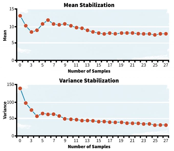
Variance Stabilization

You will need to make a decision regarding how many samples are sufficient to estimate variance for a monitoring protocol. Too few samples and the estimate may be unusually high and lead to an inability to detect differences. Too many samples and you are not being efficient with time and resources. One approach to understanding when sampling intensity is sufficient to provide a reasonable estimate of variance is to plot variance over number of samples (figure 6.1). If you want to estimate the mean and variance for a set of values, one might ask how many data points would be needed to develop a reasonable estimate of variance and a mean. Variances and means fluctuate among just a few samples, but stabilize eventually; at some point additional data are not likely to appreciably change the estimate. In the examples above (figure 6.1), variance stabilizes at about 10-15 samples and the estimate of the mean stabilizes at about 15 samples. Clearly using less than 10 samples could lead to a poor estimate of the mean and variance. More than 30 samples are probably not necessary.

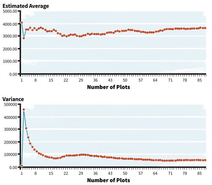
In Figure 6.2, estimates of dead wood from four 50-m transects at sample plots in young Douglas-fir stands show a high degree of variability over sample size and stabilization is observed only after a large number of plots are used in the analysis. Given such a large sample size needed to characterize the mean and variance, one would have to ask if some other indicator of this habitat element might be more efficiently characterized. For some habitat elements and populations that are highly patchy in nature, use of variance stabilization may be problematic because jumps in variance may occur as sampling efforts encounter new patches.

Spatial Patterns

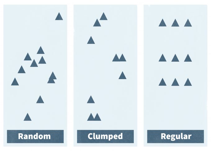
Populations and individuals can be dispersed throughout a habitat or a landscape in various patterns. Monitoring protocols must incorporate species-specific patterns in density and distributions. The three basic population spatial patterns are random, clumped, and regular (Figure 6.3; Curtis and Barnes 1988, Krebs 1989). Random dispersion is found in populations in which the spacing between individuals is irregular, and the presence of one individual does not directly affect the location of another individual. Clumped populations are characterized by patches or aggregations of individuals, and the probability of finding one individual increases with the presence of another individual. Regularly distributed populations have individuals that are distributed more or less evenly throughout an area, and the presence of one individual decreases the probability of finding another nearby individual.

The spatial distribution within populations is an important constraint on sampling designs. A number of factors influence the distribution of individuals across a habitat or landscape. Factors such as resource distribution (e.g., water, food, and cover) and habitat quality can affect the dispersion of individuals and populations (McComb 2007). A random distribution is often found in species that are dependent on ephemeral resources. Species that depend on temporary or seasonal resources may exhibit different types of distribution at different points in their life histories. In vertebrates, social behavior and territoriality can affect distribution. Highly territorial species tend to follow a regular distribution, while more gregarious and colonial nesting species tend to occur in clumps (Curtis and Barnes 1988, Newton1998). In addition, the scale of observation is critical in determining the distribution of a population. Populations may appear regularly distributed at a fine scale, such at the site level, but may show a more random or clumped distribution throughout part or all of their geographic range.

Spatial patterns of organisms and populations can complicate sampling design, but there are a number of techniques to address these constraints. Nested quadrat sampling is often used to define a species-area curve for a population or community of organisms (Krebs 1989). The number of species will expectedly rise as the size of the quadrats increase, but a plateau in species number should eventually be reached within a patch type. This plateau is considered the minimum sampling area for that community. This technique has been used successfully for plant communities (Goldsmith and Harrison 1976). However, quadrats are not natural sampling units and one must decide on a number of factors including size, shape, and number of quadrats. Refer to species area curves in the previous chapter to understand how numbers and sizes of plots can influence results. .

A useful approach for determining the spatial distribution of a population is “plotless sampling”. There are two general approaches to plotless sampling (Krebs 1989):

1. select random organisms and measure distance to nearest neighbors
2. select random points and measure distance from each point to nearest organisms

Plotless sampling has two major advantages. First, if the spatial pattern of the population is random, one can use plotless sampling to estimate the density of the population. Conversely, if the population density is known then one can determine the spatial pattern of that population. Both of these applications may prove valuable in the preliminary stages of monitoring. A first step is to estimate if a population has a random, clumped or regular distribution; approaches for estimating these distributions are given in Table 6.1.

Temporal Variation

Spatial variation is a critical limitation of successful monitoring, but sample design must also consider temporal fluctuations in populations. A sampling design that does not emphasize a dynamic and repeatable monitoring scheme will not be able to accurately estimate populations or their response to management.

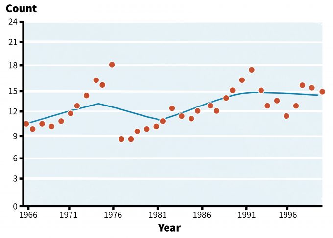
The temporal variation observed in populations is often the result of environmental variation (Akcakaya 1999). Environmental changes will have both direct and indirect effects on populations. Although we can often calculate probabilities regarding environmental fluctuations based on past records and averages (e.g., rainfall, flooding, etc.), it is often difficult, if not impossible, to predict when these changes might occur. In cases were population rates and demographics depend on environmental variables, population fluctuations are likely to occur (Akcakaya 1999). Sometimes these environmental changes can indirectly influence populations through predator densities, herbivory, sedimentation, nest predation, food resource availability, and cover. For example, a study on acorn production by oaks found that populations of white-footed mice, eastern chipmunks, and gray squirrels were significantly correlated with annual fluctuations in acorn crop (McShea 2000). In addition, these changes in small mammal populations were correlated to the nesting success of several ground-nesting birds. In eastern North America, Carolina wrens suffered a population crash following several severe winters in the mid 1970s (Figure 6.4; Barker and Sauer 1995; Sauer et al. 2001).

Analysis and interpretation of long-term monitoring should recognize and evaluate the effects of these patterns on population data. Monitoring over extended time periods and careful documentation of environmental changes (including management actions) is the only effective method for determining the change and status of a population.

Cost

A proper sampling design emphasizes cost-effectiveness, and improves the interpretation and presentation of results. Knowledge of the sample design promotes understanding and communication between project leaders and administrators, and further elucidates the critical goals of the program. Conversely, failure to consider a proper sampling design can reduce monitoring efficiency, inflate costs, and lead to inaccurate results. The inventorying and monitoring process consists of a hierarchy of decisions and events (see Chapter 5 and Jones 1986). Following the hierarchy of planning decisions, as well as constructing a reliable conceptual model, will allow managers to construct a cost-efficient sampling scheme. These decisions and goals will also dictate which type of inventory method is appropriate. Different monitoring techniques vary in their costs and intensity. For example, inventories relying on presence/not-detected data can be inexpensive because personnel with minimum training can sample fairly large areas. Comparatively, monitoring which relies on relative abundance or absolute abundance data (e.g., mark-recapture studies) demands highly skilled personnel and are generally more site-intensive. Thus, a proper sampling design, constructed through a hierarchy of decisions and input, is critical to limiting costs and collecting relevant data.

Stratification of Samples

Stratified random site selection can be an excellent method for limiting bias and collecting representative data. Although this topic will be discussed in greater detail in Chapter 11, considering stratification in your monitoring design is an important step. A stratum is an aggregation of mapping units that have similar abiotic or biotic characteristics (Jones 1986). Selecting appropriate strata is a critical step in habitat type and study site classification. In many cases, strata are based on existing vegetation and landforms. However, like many aspects of habitat assessment, strata selection can also be species-specific. For example, if it is important to collect data on a particular species, a stratum can be created that encompasses several of the habitat components that are necessary for that species. Stratification of habitats can be based on dominant or subdominant vegetation types, topographical characteristics, soil composition, ichthyologic provinces, or management areas. However, monitoring efforts and sampling is designed to be repeatable and creating strata based on vegetation can be problematic since these habitat boundaries may change over time (e.g., succession). If the characteristics used to create strata are variable over time, such as vegetation types, then it is may be necessary to reevaluate strata classification, boundaries, and criteria every year.

Adaptive Sampling

Quite often during surveys of rare plants or animals, the species of interest is observed on very few of the sampling units, and units where the species is detected are in close proximity. Many common species also have a tendency to occur in population clusters because of dispersal mechanisms, behavior patterns (e.g., herding, colonialism), or habitat associations. Under these conditions, it is predictable that surveys conducted according to conventional designs will expend most of the sampling effort at locations where the species is unobserved. Adaptive sampling designs offer an approach to concentrate sampling units in the vicinity of population clusters, thus improving the efficiency of parameter estimation. The theoretical origins of adaptive sampling extend back at least 50 years (Wald 1947, Zacks 1969) and S.K Thompson has written extensively on the application of adaptive sampling designs to plant and wildlife surveys (Thompson and Ramsey 1983, Thompson 1990, Thompson 1992, Thompson and Seber 1996). Adaptive cluster sampling has been applied to surveys of rare trees (Roesch 1993), freshwater mussels (Box et al. 2002), tailed frogs (Vesely and Stamp 2001), among other species and assemblages.

Adaptive cluster sampling refers to designs in which sample selection depends on the values of counts or other variables observed during the course of the survey. Initially, a probability procedure is used to select a set of sampling units in the study area. When any of the selected units satisfy some predetermined criterion, additional units are sampled in the vicinity of the qualifying unit. Sampling is extended until no further units satisfy the criterion. Typically the criterion is a count value of the target species.

For rare or highly aggregated populations, adaptive cluster sampling can greatly increase the precision of population size or density estimates when compared to a simple or stratified random design of equal cost (1992). Adaptive cluster sampling can be applied to surveys conducted on quadrats, belt transects, variable circular plots, among other types of sampling units. Thompson and Seber (1996) provide a comprehensive review of adaptive sampling designs and data analysis. There are two different considerations that may limit the applicability of adaptive sampling designs for some inventory and monitoring studies. First, adaptive sample selection may cause biases in conventional estimators for the population mean, variance, and total population size. Unbiased estimators have been described for simple and stratified adaptive sampling designs, but cannot be automatically computed with commonly-used statistical software. Calculation of design-unbiased estimators for adaptive sampling designs requires a thorough understanding of statistics and the ability to program the estimators into one of the advanced statistical software packages (e.g., SAS^®, S+^®). A statistical consultant can aid in developing analytical methods appropriate for adaptive sampling, and provide similar assistance in performing data analysis. The second consideration in planning for adaptive sampling is the operational uncertainty surrounding the number of sampling units required for the survey. Unlike conventional designs in which the sample size is typically determined before starting fieldwork, there is no precise knowledge prior to data collection as to the number of units that will trigger secondary surveys. This uncertainty can be minimized by conducting pilot studies to estimate the mean and variance for sample sizes. Alternatively, survey protocols can limit the maximum number of sampling units visited in a study area, after making appropriate modifications to the population estimators.

Peer Review

Once a sampling design has been developed based on existing data or a pilot study, there is still some doubt that the data collected as part of the monitoring effort will adequately address all potential biases or inherent fluctuations in conditions over time. One step that can be extremely valuable in the development of a protocol is to draft the sampling design, providing the preliminary data analyses and rationale for indicators selected, sampling intensity, effect sizes, and power. This draft should be reviewed by both a statistician and an expert on the biology of the organism(s) and ecosystem(s). Recall that statistics are merely a tool to help make decisions. The design must be statistically sound, but it must also be biologically meaningful. External review of the design can help to identify features of the sampling design that may limit the usefulness of the data in the analytical phase of the monitoring program. It is much better to be thorough in development of the design phase and minimize the risk of making errors now then to find out after a year or more of data collection that the results are biased, not independent, or too variable to make inferences.

Summary

In addition to developing clear objectives, having a random sample, and having adequate power in your design to detect trends, the monitoring plan should include a framework for analyzing and interpreting the data. Existing data from other studies or a pilot study may be particularly useful when estimating detectability, variance in potential indicators, estimating costs of monitoring, maximizing efficiency during adaptive sampling tests, and estimating spatial and temporal patterns in habitat elements or populations. These and other ancillary data may aid in the identification of strata as monitoring plans are designed. Stratified random site selection can be an excellent method for limiting bias and collecting representative data. For rare or highly aggregated populations, adaptive cluster sampling can greatly increase the precision of population size or density estimates when compared to a simple or stratified random design of equal cost. Finally, the monitoring plan should be subjected to rigorous peer review prior to implementation.

References

Akçakaya, H.R., M.A. Burgman, and L.R. Ginzburg. 1999. Applied population ecology: principles and computer exercises using RAMAS EcoLab. Second Edition. Sinauer Associates, Inc., Sunderland, Massachusetts, USA.

Barker, R.J., and J.R. Sauer. 1995. Statistical aspects of point count sampling.   Pages 125-130 in C.J. Ralph, J.R. Sauer, and S. Droege, eds. Monitoring Bird Populations by Point Counts. USDA Forest Service General Technical Report PSW-GTR-149.

Besag, J E. and J.T. Gleaves. 1973. On the detection of spatial pattern in plant communities. Bull. Int. Statist. Inst. 45:153-158.

Box, J.B., R.M. Dorazio, and W.D. Liddell. 2002. Relationships between streambed substrate characteristics and freshwater mussels (Bivalvia: Unionidae) in coastal plain streams. Journal of the North American Benthological Society 21:253-260.

Burnham, K.P., D.R. Anderson and J.L. Laake. 1980. Estimation of density from line transect sampling of biological populations. Wildlife Monographs 72:202pp.

Byth, K. and Ripley, B.D. 1980. On sampling spatial patterns by distance methods. Biometrics 36:279-284

Chambers, C.L, W.C. McComb, and J.C. Tappeiner. 1999. Breeding bird responses to 3 silvicultural treatments in the Oregon Coast Range. Ecological Applications 9:171-185

Clark, P.J., and F. Evans. 1954. Distance to nearest neighbor as a measure of spatial relationships in populations. Ecology 35:445-453.

Cottam, G., and J.T. Curtis. 1956. The use of distance measures in phytosociological sampling. Ecology 37:451-460.

Curtis, H. and N.S. Barnes. 1988. Biology. 5th ed. New York: Worth Publishers. 1050pp.

Gibbs, J.P., and P. Ramirez de Arellano. 2007. Program MONITOR: Estimating the Statistical Power of Ecological Monitoring Programs. Version 10.0. URL: www.esf.edu/efb/gibbs/monitor/monitor.htm

Goldsmith, F.B., and C.M. Harrison. 1976. Description and analysis of vegetation. Pages 85-157 in S.B. Chapman, editor. Methods in plant ecology. Blackwell Scientific. Oxford, United Kingdom.

Hinds, W.T. 1984. Towards monitoring of long-term trends in terrestrial ecosystems. Environmental Conservation 11:11-18.

James, F.C., C.E. McCulloch, and D.A. Wiedenfeld. 1996. New approaches to the analysis of population trends in land birds. Ecology 77:13-27.

Jones, K.B. 1986. Data types. Pages 11-28 in A.Y. Cooperrider, R.J. Boyd, and H.R. Stuart, editors. Inventorying and monitoring wildlife habitat. USDI Bureau of Land Management, Denver, Colorado, USA.

Krebs, C. J. 1989. Ecological methodology. Harper Collins, New York, NY. 654 pp.

McComb, B.C. 2007. Wildlife habitat management: Concepts and applications in forestry. Taylor and Francis Publishers, CRC Press, Boca Raton, FL. 319pp

McShea, W.J. 2000. The influence of acorn crops on annual variation in rodent and bird populations. Ecology 81:228-238.

Newton, I. 1998. Population limitations in birds. Academic Press, Inc., New York, New York, USA.

Noss, R.F. 1990. Indicators for monitoring biodiversity: a hierarchal approach. Conservation Biology 4:355-364

Ricker, W.E. 1975. Computation and interpretation of biological statistics of fish populations. Bulletin of the Fisheries Research Board of Canada. No. 191. 382pp.

Roesch, F.A., Jr. 1993. Adaptive cluster sampling for forest inventories. Forest Science 39: 655-669.

Sauer, J.R., J.D. Nichols, J.E. Hines, T. Boulinier, C.H. Flather, and W.L. Kendall. 2001.   Regional patterns in proportion of bird species detected in the North American Breeding Bird Survey Pages 293-296 In R. Field, R.J. Warren, H. Okarma, and P.R. Sievert, editors. Wildlife, land, and people: priorities for the 21^st century. Proceedings of the 2^nd. International Wildlife Congress. The Wildlife Society, Bethesda, MD, USA.

Sauer, J.R., Peterjohn, B.G., and Link, W.A. 1994. Observer differences in the North American Breeding Bird Survey. Auk 111:50-62.

Sauer, J.R., J.E. Hines, and J. Fallon. 2007. The North American Breeding Bird Survey, Results and Analysis 1966 – 2006. Version 10.13.2007. USGS Patuxent Wildlife Research Center, Laurel, MD.

Seber, G.A.F. 1982. Estimation of animal abundance and related parameters. Oxford Univ. Press, New York, 654pp.

Thomas, L. 1996. Monitoring long-term population change: why are there so many analysis methods? Ecology 77:49-58.

Thompson, S.K. 1990. Adaptive cluster sampling. J. Am. Stat. Assoc. 85, 1050-1059

Thompson, S.K. 1992. Sampling. Wiley, New York. 343pp.

Thompson, S.K., and F.L. Ramsey. 1983. Adaptive sampling of animal populations. Technical Report 82. Dept. of Statistics, Oregon State University, Corvallis, OR.

Thompson, S.K. and G.A.F. Seber. 1996. Adaptive Sampling. John Wiley, New York. 270pp.

Vesely, D.G. and J. Stamp. 2001. Report on surveys for stream-dwelling amphibians conducted on the Elliott State Forest, June-September, 2001. Report prepared for the Oregon Department of Forestry. Pacific Wildlife Research, Corvallis, OR.

Wald, A. 1947. Sequential Analysis. John Wiley, New York.230pp.

Zacks, S. 1969. Bayes sequential designs of fixed size samples from finite populations. Journal of the American Statistical Association.64:1342-1349.