5 Designing a Monitoring Plan
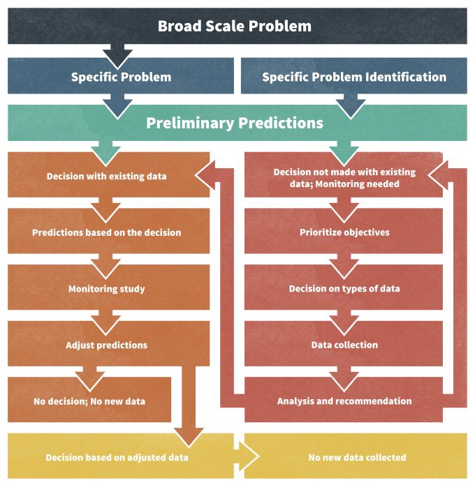
Design of a monitoring plan is a process (Figure 5.1) that will ideally lead you through problem identification, to development of key questions, a rigorous sampling design, and analyses that can assign probabilities to observed trends. Finalizing a plan designed as an outcome of this process is a precursor to initiation of data collection. This is probably the single most important step in the monitoring plan. Once you have decided on the design for the monitoring plan, and begun collecting data, there is strong resistance to changing the plan because many changes will render the data collected thus far of less value. So design it correctly from the outset to minimize the need for changes later.
Articulating Questions to Be Answered
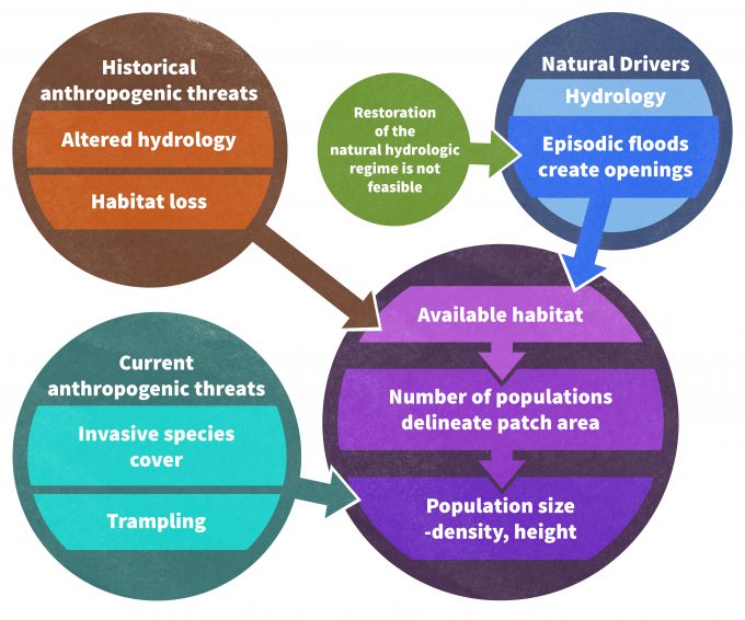
It is important to view monitoring as comparable in many ways to conducting a scientific investigation. The first step in the process is to develop a conceptual framework for our current understanding of the system, complete with literature citations to support assumptions. Clearly no monitoring program will have all of the information needed to completely develop a conceptual model for the system under consideration. Available information will have to be extracted from the literature, from other systems and from expert opinion. Nonetheless, the conceptual model needs to be developed in order to identify the key gaps in our knowledge and allow a clear articulation of the most pertinent questions (Figure 5.2).
As you develop the monitoring plan you should pay particular attention to some terms that are commonly used to define the problem and the approach. Within the context of land management and biodiversity conservation, these terms might guide you to the kind of monitoring design that you will choose to use.
These terms relate to the experimental design:
- Cause and effect – Will you be able to infer the cause for observed changes?
- Association or relationship – Will you be able to detect associations between pairs of variables such as populations and changes in area of a habitat type?
- Trend or pattern – Will patterns over space and/or time be apparent?
- Observation or detection – What constitutes having ‘observed’ an individual?
These terms relate to the response variable that you will measure to assess one of the above:
- Occurrence — Was the species present, absent or simply not detected?
- Relative abundance – Did you observe more individuals in one place or time than another?
- Abundance – How many individuals per ha (or square km) are estimated to be present?
- Fitness – Is the species surviving or reproducing better in one place or time than another?
These terms relate to the scope of inference for the effort:
- Stand, harvest unit, field, pasture, project, farm, district, watershed, forest, region — defines the grain and extent of the spatial scale of the potential management effects
- Home range, sub-population, geographic range, stock, clone — defines the grain and spatial extent associated with the focal species.
- Frequency of management or exogenous disturbances affecting the system — helps define the sampling interval
- Return interval between disturbances or other events likely to effect populations of the focal species — helps define the duration of the monitoring framework
- Disturbance intensity or the degree of change in biomass or other aspects of the system as a function of management or exogenous disturbances — helps to understand how effect sizes should be defined and hence the sampling intensity sufficient to detect trends or differences.
Once you have articulated questions based on the conceptual model for the system, then you should use terms from each of the groups above to further define the monitoring plan. Detail and focus are important aspects of a well-designed monitoring system. Use of vague or unclear terms, broad questions, or unclear spatial and temporal extents will increase the risk that the data collected will not adequately address the key questions at scales that are meaningful. Further, clearly articulated questions not only ensure that data collected are adequate to address specific key knowledge gaps or assumptions, they also provide the basis for identifying thresholds or trigger points which initiate a new set of management actions.
If the above terms are considered when the monitoring plan is being designed, and trigger points for management action are described clearly prior to monitoring, then it should be apparent that the universe of questions that could be addressed by monitoring is very broad. Of course, your challenge is to identify the key questions that address the key processes and states in an efficient and coordinated manner over space and time. Given a conceptual model developed for a system, there is a range of questions that could be addressed through monitoring. Prioritization of these questions allows the manager to focus time and money on the key questions.
Inventory, Monitoring, and Research
The questions of concern may be addressed using inventory, monitoring or research approaches (Elzinga et al. 1998). Inventory is an extensive point-in-time survey to determine the presence/absence, location or condition of a biotic or abiotic resource. Monitoring is a collection and analysis of repeated observations or measurements to evaluate changes in condition and progress toward meeting a management objective. Detecting a trend may trigger a management action. Research has the objective of understanding ecological processes or in some cases determining the cause of changes observed by monitoring. Research is generally defined as the systematic collection of data that produces new knowledge or relationships and usually involves an experimental approach, in which a hypothesis concerning the probable cause of an observation is tested in situations with and without the specified cause. Some biologists make a strong case that the difference between monitoring and research is subtle and that monitoring should also be based on testable hypotheses. Nonetheless, these three approaches to gaining information are highly complementary and not really very discrete. And all three approaches are needed to effectively manage an area without unnecessary negative effects.
Are Data Already Available?
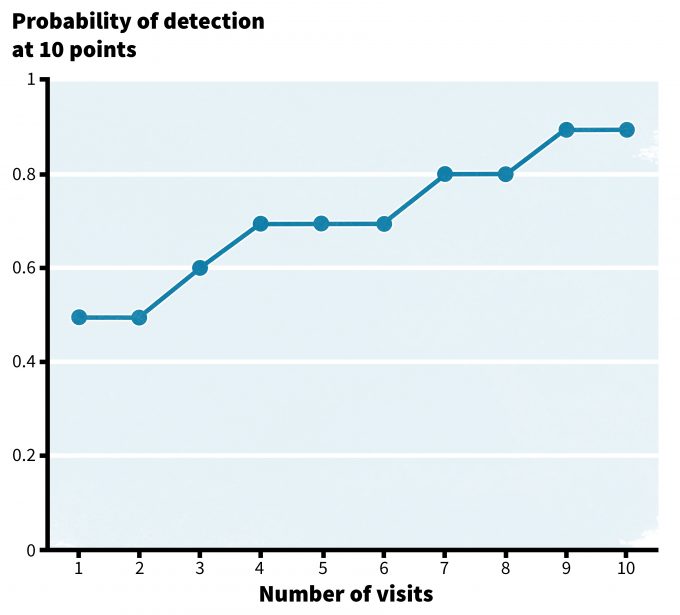
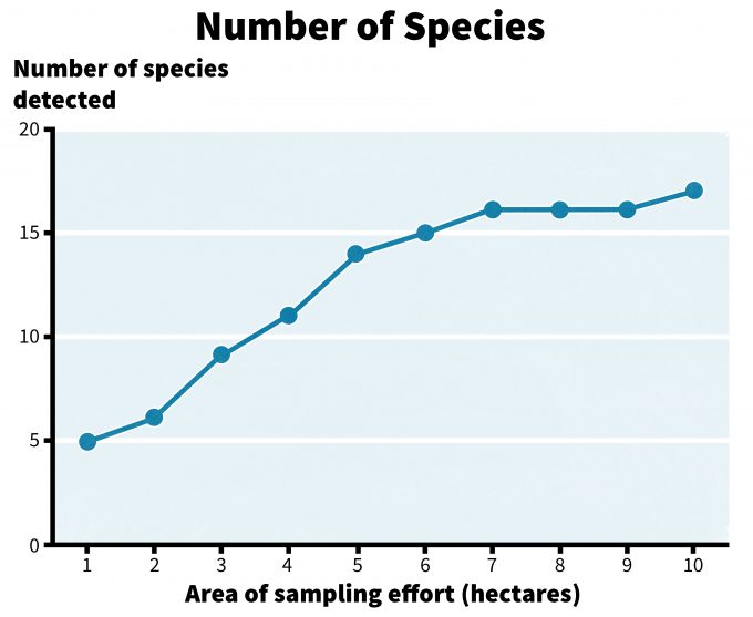
You may already have some data that have been collected previously or from a different area. Can you use these data? Should you? What constitutes adequate data already in hand, or how do we know when data are adequate to address a question? Well, that depends on the question! For example, if we want to be 90% sure that a species does not occur in a patch or other area to be managed in some manner in the next year, how many samples are required to reach that level of confidence? Developing a relationship between the amount of effort expended and the probability of detecting species ‘x’ in a patch, can provide insight into the level of effort needed to detect a species 90% of the time when it indeed does occur in the patch. This requires multiple patches and multiple samples per patch over time to place confidence intervals on probabilities (Figure 5.3). Where multiple species are the focus of monitoring, a species-area chart can be quite helpful. For example in Figure 5.4, sampling an area less than 7 hectares in size is not likely to result in a representative list of species for the site.
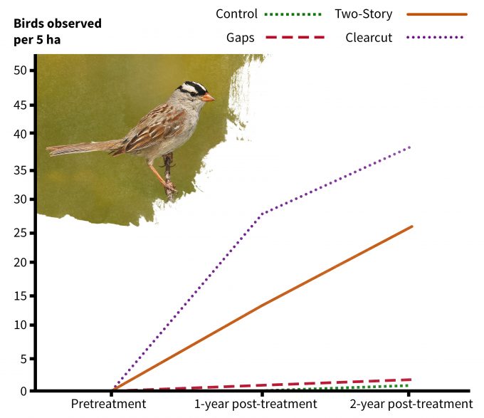
These sorts of questions require quite different data than would be required to answer the question: What are the effects of management ‘x’ on species ‘y’? Note that the term’ effect’ is used in this example, so the experimental design is ideally in the form of a manipulative experiment (Romesburg 1981). In this case, we would want to have both pre- and post-treatment data collected on a sample of patches that do and do not receive treatment. In the following example, two of the treatments clearly had an effect on the abundance of white-crowned sparrows in managed stands in Oregon (Figure 5.5). Results such as these are base don specific questions. It is the development of the question that is important and the question should evolve from the conceptual model of the system. Clearly the development of a conceptual model to describe the system states, processes, and stressors, should be based to the degree possible on data. So although currently available data are valuable, they must address the question of interest in a manner that is consistent with the conceptual model. It is important to recognize that not all data are equal. Consider the following questions when evaluating the adequacy of a data set to address a question or to develop a conceptual framework:
- Are samples independent? That is, are observations in the data set representing management units to which a treatment has been applied? Using a forest example, taking 10 samples of densities of an invasive species from one patch is not the same as taking one sample from 10 patches (Hurlbert 1984). In the former example, the samples are sub-samples of one treatment area, in the latter there is one sample in each of 10 replicate units. If the species under consideration has a home range that is less than the patch size, then the patches are reasonably independent samples. If the species under consideration has a home range that spans numerous patches, then the selection of patches to sample should be based on ensuring to the degree possible that one animal is unlikely to use more than one managed patch.
- How were the data collected? What sources of variability in the data may be caused by the sampling methodology (e.g., observer bias, inconsistencies in methods, etc.)? If sample variability is too high because of sampling error, then the ability to detect differences or trends will decrease. Further if the samples taken are biased then the resulting conclusions will be biased and decisions made based on those conclusions may be inappropriate.
- Were sites selected randomly? If not, then there may be (likely is) bias introduced in to the data that should raise doubts in the minds of the scientists, managers and stakeholders with regard to the accuracy of the resulting relationships or differences.
- What effect size is reasonable? Even a well designed study may simply not have the sample size adequate to detect a difference or relationship that is real simply because the study was constrained by resources, rare responses, or other factors that increase the sample variance and decrease the effect size that can be detected. Again, how this is dealt with depends on the question being asked. Which is more important, to detect a relationship that is real or to say that there is no relationship when there really isn’t? In many instances, where monitoring is designed to detect an effect of a management action, the former is more important. In that case, the alpha level used to detect differences or trends may be increased (from say 0.05 to 0.10), but you will be more likely to say a relationship is real when it is really not. Alternatively, you may want to use Bayesian analysis or meta-analysis to examine the data and see if these techniques shed light on your question. See Chapter 11 for a more in-depth discussion of these analytical techniques.
- What is the scope of inference? From what area were samples selected? Over what time period? Are the results of the work likely to be applicable to your area? As the differences in the conditions under which the data were collected increase compared to the conditions in your area of interest, the less confidence you should have in applying the results in your context.
If, after considering the above factors, you feel that the data can be used to reliably identify known from unknown states and processes in the conceptual model, then you should have a better idea where the model relies heavily on assumptions, weak data, or expert opinion. These portions of the conceptual model should rise to the top during identification of the question that monitoring should be designed to address.
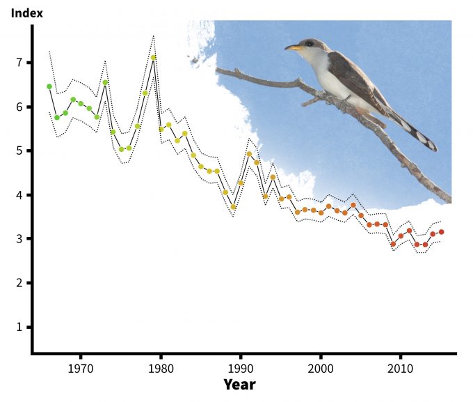
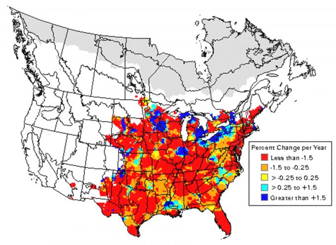
Provided that the cautions indicated above are explored, it is reasonable and correct to use data that are already available to inform and focus the questions to be asked by a monitoring plan. Existing data are commonly used to address questions. For instance, Sauer et al. (2001) provided a credibility index that flags imprecise, small sample size, or otherwise questionable results. Yellow-billed cuckoos have shown a significant decline in southern New England over the past 34 years (Figure 5.6), but the analysis raises a flag with regards to credibility because of a deficiency in the data associated with low abundance (<1.0 bird/route). Further, an examination of the data would indicate that the one estimate in 1966 may be an outlier and may have an over-riding effect on the results. In this example, it would be useful to delete the 1966 data and re-run the analyses to determine if the relationship still holds. Regardless of the outcome of this subsequent analysis, the data will likely prove useful when developing a conceptual model of population change for the species. When the proper precautions are taken, such data may allow the manager to focus on more specific questions with regard to a monitoring plan. For instance, within the geographic range of the species, what factors may be causing the predicted declines? The BBS data reveals that the species is not predicted to have declined uniformly over its range (Figure 5.7). This information may provide an opportunity to develop hypotheses regarding the factors causing the declines.
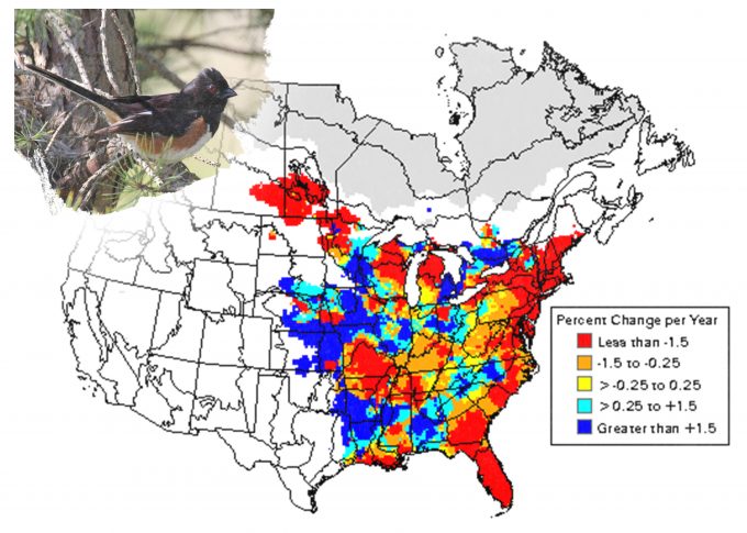
Recorded trends in abundance for eastern towhees (fig 5.8) provide another clear example. In this case, declines are apparent throughout the entire northeastern United States. Based on our knowledge of changes in land use in the northeast and the association of this species with early successional scrub vegetation, we would hypothesize that the declines are a direct result of the re-growth of the eastern hardwood forests and subsequent loss of shrub-dominated vegetation. Indeed, monitoring the reproductive success of the species prior to and following vegetation management designed to restore shrub vegetation might allow detection of a cause and effect relationship that would lead to a change in monitoring for the species over the northeastern portion of its range. If changes in abundance were related to changes in land cover (and not to parasitism by brown-headed cowbirds or other effects), then an alternative monitoring framework could be developed. Infrequent monitoring of populations with frequent monitoring of the availability of the habitat elements important to the species (shrub cover) may be adequate to understand the opportunities for population recovery (or continued decline). This reveals the potential benefits of applying previously generated data: generally costs associated with monitoring habitat availability are less than costs associated with monitoring populations or population fitness, so if a cause and effect relationship were detected between vegetation and bird populations, then managers could see considerable savings in their monitoring program.
In summary, although there are general guidelines with regards to what constitutes reliable data, adequate data for one question may be inadequate for another. Use of existing data and an understanding of data quality can allow development of a conceptual model where states, processes and stressors can be identified with varying levels of confidence. Those factors that are based on assumptions or weak data and which seem quite likely to be influencing the ability to understand management effects, should become the focus when developing the questions to be answered by the monitoring plan.
Types of Monitoring Designs
Before we provide examples of the types of monitoring designs, recall that there are several main points consistent among all designs:
- Are the samples statistically and biologically independent?
- How were the data collected? What sources of variability in the data may be caused by the sampling methodology (e.g., observer bias, inconsistencies in methods, etc.). If sample variability is too high because of sampling error, then the ability to detect differences or trends will decrease.
- Were sites selected randomly? If not, then there may be (likely is) bias introduced in to the data that should raise doubts in the minds of the plan developers with regard to the accuracy of the resulting relationships or differences.
- What effect size is reasonable to detect?
- What is the scope of inference?
Once these questions are addressed, then there are additional considerations depending on the type of monitoring that will be conducted.
Incidental Observations
Opportunistic observations of individuals, nest sites, or habitat elements can be of some value to managers, but often are of not much use in a monitoring framework except to provide preliminary or additional information to a more structured program. For instance, global positioning system (GPS) locations of a species observed incidentally over a three-year period could be plotted on a map and some information can be derived from the map (known locations). The problem with using these data points in a formal monitoring plan is that they are not collected within an experimental design. There undoubtedly are biases associated with where people are or are not likely to spend time; with detectability among varying vegetative, hydrologic, or topographic conditions; and detectability of different age or sex cohorts of the species. Consequently this information should be maintained, but rarely would it be used as the basis for a formal monitoring design.
Inventory designs
Assume that you are concerned that proposed management actions will impact a species that could be present in your management area. How sure do you want to be that the species occurs on the proposed management area? Do you want to know with 100% confidence? Or can you be 95% sure? 90%? The answer to that question will dictate both the sampling design and the level of intensity with which you inventory the site to estimate presence and (presumed) absence.
First, and foremost, you will need to decide what will constitute an independent sample for this design. Are you most concerned that a species does/does not occur on a proposed set of managed patches? If so, sampling of all, or a random sample of proposed managed patches will be necessary. But what if the managed patches are clustered and the species of interest has a home range that overlaps some of the managed patches? Are you likely to detect the same individual on multiple units? If so, is it necessary to detect it on all units within the species home range? Not likely. For species with home ranges larger than a managed patch, you will probably want to sample an area of sufficient size and intensity to have a high probability of detecting the species within that home-range-sized area. Randomly selected areas should be independent with respect to minimizing the potential for detecting the same individual on multiple sites. Random sampling of sites then would be constrained by eliminating those sites where double counting of individuals is likely.
In an inventory design generally you wish to be ‘x’ confident that you have detected the species if it is really there. Consequently a pilot study that develops the relationship between the probability of detecting an individual and sampling intensity will be critical. Consider use of remotely activated recorders for assessing presence/absence of singing male birds in an area. How many mornings would you need at each site to detect a species that does occur at the site? A pilot study may entail 20 or 30 sites (more if the species is rare) to allow you to graph the cumulative detections of the species over the number of mornings sampled (Figure 5.2). Eventually an asymptote should be reached and one could then assume that additional sampling would not likely lead to additional detections. Confidence intervals can be placed on these estimates, and the resulting estimated level of confidence in your ability to detect the species can (and should be) reported. Results of pilot work (or published data) such as this often allow more informative estimates of the probability of a species occurring in an area to be generated in the subsequent sampling during the monitoring program. This is especially the case when estimated levels of confidence can be applied to the monitoring data.
There are several issues to consider when developing a monitoring plan that is designed to estimate the occurrence or absence of a species in an area. First, the more rare or cryptic the species, the more samples that will be needed to assess presence, and the sampling intensity can become logistically prohibitive. In that case other indicators of occurrence may need to be considered.
Consider the following possibilities when identifying indicators of occurrence in an area:
- Direct observation of a reproducing individual (female with young)
- Direct observation of an individual, reproductive status unknown (Are these first two indicators of occurrence or something different, such as indicators that management will have an impact?)
- Direct observation of an active nest site
- Observation of an active resting site or other cover
- Observation of evidence of occurrence such as tracks, seeds, pollen
- Identification of habitat characteristics that area associated with the species
Any of the above indicators could provide evidence of occurrence and hence potential vulnerability to management, but the confidence placed in the results will decrease from number 1 to number 6 for most species based on the likelihood that the fitness of individuals could be affected by the management action.
Finally we strongly suggest that statistical techniques that include data that influence the probability of detection be used. MacKenzie et al. (2003) provide a computer program PRESENCE that uses a likelihood-based method for estimating site occupancy rates when detection probabilities are <1 and incorporates covariate information. They also provide information on survey designs that allow use of these approaches (MacKenzie and Royle 2005).
Status and trend monitoring designs
Long-term monitoring of populations to establish trends over time are coordinated over large areas under several efforts. For instance the US Geological Survey (USGS) Biological Resources Division (BRD) has been involved in monitoring birds and amphibians, as well as contaminants and diseases that may affect populations of these species. Results of these efforts as well as supporting research information provides the basis for understanding why we might be seeing trends in biological resources over large areas (e.g., USGS Status and Trends Reports). Such monitoring systems provide information on changes in populations, but they do not necessarily indicate why populations are changing. For instance, consider the changes in American woodcock populations over a 27-year period (Figure 5.9).
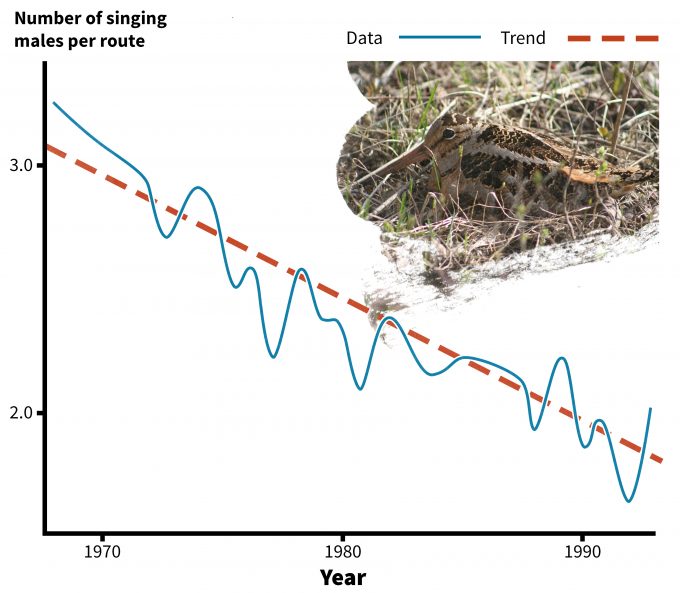
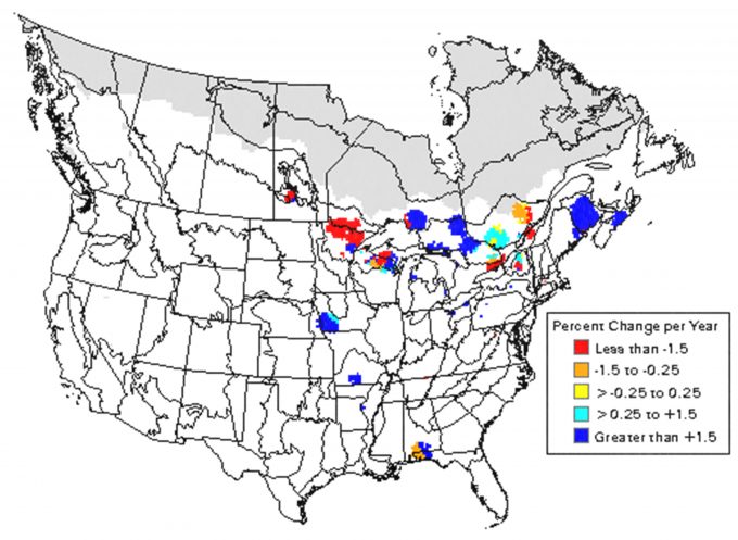
Clearly, the number of singing males has declined markedly over this time period. This information is very important in that it indicates that additional research may be needed to understand why the changes have occurred. Are singing males simply less detectable than they were in 1968? Are populations actually declining? If so, are the declines due to changes in habitat on the nesting grounds? Wintering grounds? Migratory flyways? Is the population being over-hunted? Are there disease, parasitism, or predator effects that are causing these declines? Are these declines uniform over the range of the species or are there regional patterns of decline? Analysis of regional patterns indicates that the declines may not be uniform (Figure 5.10). .Indeed, declines in woodcock numbers are apparent in the northeastern U.S., but not throughout the Lake States. So it would seem that causes for declines are probably driven by effects that are regional. Woodcock provide a good example of the need to consider the scope of inference in design of a status and trends monitoring plan. The Breeding Bird Survey data indicate that there are areas where declines have been significant, and the work by Bruggink and Kendall (1997) indicate that the magnitude of the declines in some areas are perhaps even greater than might be indicated by the regional analyses. Such hierarchical approaches provide opportunities for understanding the potential causes for change in abundance or relative abundance of a species at a more local scale. This insight may allow managers to be more effective in identifying the causes of declines at local scales in a manipulative manner where local, intensive monitoring and research can result in the discovery of a cause and effect relationship.
Consequently the design of a status and trends monitoring plan should carefully consider the scope of inference, generally a large portion of the geographic range, and may necessitate the coordination of monitoring over large areas and multiple agencies. Site-specific status and trends analyses will probably be of limited value in many instances because the fact that species ‘x’ is declining at site ‘y’ is probably not as important as knowing why the species is declining at site ‘y’. In addition, for those species with a meta-population structure (ones with subpopulations maintained by dispersal and recolonization), observed changes at local sites may simply reflect source-sink dynamics in the meta-populations and not the trend of the population as a whole. Using status and trends monitoring to detect increases or declines in abundance is perhaps best applied to identify high priority species for more detailed monitoring, or to allow development of associations with regional patterns of vegetation or urban development. These associations then allow the opportunity for a more informed development of hypotheses that can then be tested in manipulative experiments to identify causes for changes.
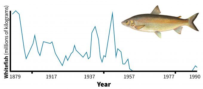
One aspect of status and trends monitoring that must be considered carefully is the sampling intensity needed to detect a change in slope over time. Consider the data in figure 5.9. Annual data were quite variable over the 27-year period, but a trend is still detectable because the slope was so steep. Annual variability caused by population fluctuations and sampling variance can prevent detection of a statistically significant change in slope. This problem is exacerbated when the slope is not so dramatic. Consider the trend for whitefish harvest in Lake Erie (Figure 5.11). Annual variability in whitefish harvest was so variable from year to year that detection of a statistically significant trend line is very difficult. Commercial harvest as an indicator of populations is clearly biased due to variability in harvest intensity, resource value and techniques. Use of traditional time-series regression analyses to detect trends may not be the best approach. Use of Bayesian analyses may be more informative (Wade 2000). Nonetheless when commercial harvests reach zero (or nearly so), a threshold is reached where dramatic action must be taken to recover the stocks. Hence there are several factors that must be considered carefully in the design of status and trends plans:
- What is the spatial scale over which you wish to understand if populations are declining or increasing? If the extent of the monitoring effort is not the geographic range of a species or sub-species, than what portion of the geographic range will be monitored and how will the information be used?
- Is the indicator (e.g., occurrence, abundance, fitness) that is selected as unbiased as possible and not likely to vary among time periods except those caused by fluctuating populations?
- Given the inherent variability in the indicator that is being used, how many samples will be needed each time period to allow detection of a slope of at least ‘x’ percent per year over time (Gibbs and Ramirez de Arellano 2007)?
- Given the inherent variability in the indicator that is being used, at what point in the trend is action taken to recover the species or reverse the trend (what is the trigger point)? Note that this must be well before the population reaches an undesirably low level, because the manager will first have to understand why the population is declining before action can be taken.
- Will the data be used to forecast results into the future? If so, recognize that the confidence intervals placed on trend lines diverge dramatically from the line beyond the bounds of the data. Forecasting even a brief period into the future is usually done with little confidence unless the underlying cause and effects are understood.
Finally, it is important to recognize that quite often when data are analyzed using time-series regression, auto-correlation among data points (the degree of dependence of one data point on preceding data) is not only likely, it should be expected. Although the chapter 11 provides extensive guidance in analyzing these data, briefly we describe why these factors must be considered during plan design.
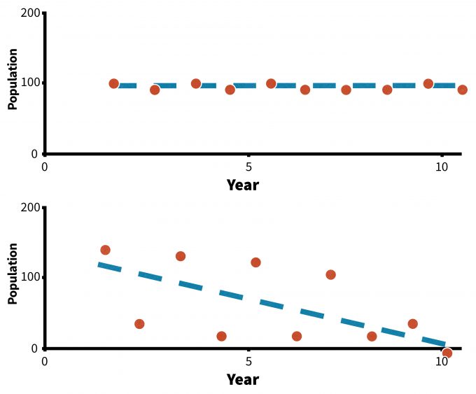
Parametric analyses are designed to reject the null hypothesis with an estimated level of certainty (e.g., we reject the null hypothesis that the slope is 0 and conclude that there is a decline). With rare species, variable indicators, or sparse data, we may lack the statistical power necessary to reject that hypothesis, even when a trend line seems apparent. In the Figure 5.12, we may choose to use alternative analyses (Wade 2000) to assess trends in sample B, or increase our alpha level, thereby increasing our likelihood of rejecting the null hypothesis. Changing alpha will increase the risk of stating that there is a trend when there really is not, however, this may be an acceptable risk. If we risk losing a species entirely or over a significant part of its geographic range, we will probably be willing to make an error that results in stating that a population is declining when it really is not. This is an important point, because two individuals approaching trend data with a different perspective (alpha level) may reach very different conclusions.
Cause and Effect Monitoring Designs
Typical research approaches will either assess associations between response variables and predictor variables, or will use a structured experimental design that will assess cause and effect. Monitoring plans can also use this approach. Consider a trend line for white-tailed deer in Alabama that showed a significant decline. Consider also that the manager had just stopped using prescribed burning to manage the area. She might conclude that the cessation of burning caused the decline. But if data from a nearby unburned area were also available and that trend line was also negative, then she might reach a different conclusion and begin looking for diseases or other factors causing a more regional decline.
If the plan being developed is designed to understand the short or long-term effects of some management action on a population, then the most compelling monitoring design would take advantage of one of two approaches to assess responses to those actions: retrospective comparative mensurative designs or Before-after Control-Impact (BACI) designs.
Retrospective Analyses and ANOVA designs
Monitoring conducted over large landscapes or multiple sites may use a comparative mensurative approach to assess patterns and infer effects (e.g., McGarigal and McComb 1995, Martin and McComb 2001). This approach allows comparisons between areas that have received management actions and those that have not and often is designed using an Analysis of Variance (ANOVA) approach. Retrospective designs that compare treated sites to untreated sites raise questions about how representativeness of the untreated sites prior to treatment. In this design, the investigator is substituting space (treated vs untreated sites) for time (pre- vs. post treatment populations). The untreated sites are assumed to be representative of the treated sites before they were treated. With adequate replication of randomly selected sites, this assumption could be justified, but often large-scale monitoring efforts are costly and logistics may preclude both sufficient replication and random selection of sites. Hence doubt may persist regarding the actual ability to detect a cause-and-effect relationship, or the power associated with such a test may be quite low. Further, lack of random selection may limit the scope of inference from the work only to the sites sampled.
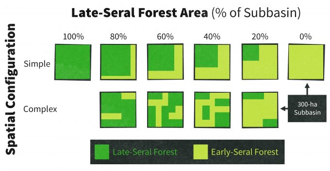
McGarigal and McComb (1995) compared bird detections among 6 levels of mature forest abundance and 2 levels of forest pattern using a retrospective ANOVA design (Figure 5.13). Logistics restricted them to only 3 replicates of each condition, and sites were selected randomly from among those available, though in most cases few options were available. Further there was the potential for areas that had been managed to have different topography, site conditions, or other factors that made those sites more likely to receive management than those sites that did not. The patterns of association between bird species and landscape conditions were significant in many instances, and consistent with what we know about the life history of the species. But despite the fact that most of the species in table 5.1 have been associated with older or closed-canopy forests in previous studies (lending support for the fact that their relative abundance should increase with increasing area of old forest) we cannot make any definitive conclusion. Rather, we can only hypothesize that these species should respond positively to increasing area of old forest. Monitoring data on these species collected over time can be used to test that hypothesis.
| ANOVA | Regression | |||
| Species | F | P | R2 (%) | P |
| Gray jay | 14.2 | <0.001 | 63 | <0.001 |
| Brown creeper | 13.4 | <0.001 | 59 | <0.001 |
| Winter wren | 8.6 | <0.001 | 53 | <0.001 |
| Varied thrush | 7.8 | <0.001 | 24 | 0.007 |
| Pileated woodpecker | 2.51 | 0.068 | 18 | 0.019 |
| Hermit warbler | 1.4 | 0.271 | 12 | 0.063 |
Before-After Control vs. Impact (BACI) designs
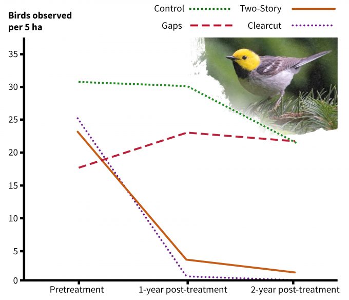
Although the BACI design is usually considered superior to the ANOVA design, BACI designs often are logistically challenging. The BACI design allows monitoring to occur on treated and untreated sites both before and after management has occurred (e.g., Chambers et al. 1999). BACI designs allow detection of cause-and-effect relationships, but within monitoring frameworks, they can often suffer from non-random assignment of treatments to sites. Often the location and timing of management actions do not lend themselves to strict experimental plans. In the following example, Chambers et al. (1999) used a BACI design experiment that included silvicultural treatments in three replicate areas on a working forest (Figure 5.14). The results from this effort again produced predictable responses, but the responses could clearly be linked to the treatments. In figure 5.5, white-crowned sparrows were not present on any of the pre-treatment sites, but were clearly abundant on the clearcut and two-story stands following treatment (vertical bars represent confidence intervals). The treatments caused a response in the abundance of this species. Conversely, hermit warblers declined in abundance on these two treatments but remained fairly constant on the control and group selection treatments (figure 5.15). Consequently we would predict that future management actions such as these would produce comparable results on this forest. However it is important to remember that the scope of inference is this one forest – extrapolation to other similar sites should be done with caution. Further, to fully understand why these changes might have been observed, ancillary data on habitat elements important to these species also could be collected and if the treatments caused changes in important habitat elements, then the reasons for the effects become clearer. These habitat relationships analyses can be particularly informative when developing predictive models of changes in abundance or fitness of an organism based on management actions or natural disturbance.
EDAM: Experimental Design for Adaptive Management
Choosing a design for monitoring can be facilitated using software specifically developed to assess statistical rigor of the plan (e.g., Program MONITOR) and software which can guide design of adaptive management efforts. Anderson (1998) developed EDAM software to guide an adaptive management experiment that may never be repeated, but instead may lead directly to economically significant management decisions. Traditional design recommendations alone may not be helpful in this scenario because manipulating design variables, such as sample size or length of the experiment, often involves very high costs. Also, various stakeholders may have different points of view concerning the impact of possible incorrect inferences (Anderson 1998). There are two versions of the EDAM model: a Before-After-Control-Impact Paired Series (BACIPS) experiment on a landscape scale, and an Analysis of Variance (ANOVA) experiment on a patch scale:
“Each model represents a management experiment on a forest ecosystem, which can be examined from different stakeholders’ points of view. Given a set of design choices, the model demonstrates all possible outcomes of the experiment and their likelihood of occurrence, with a special emphasis on their future economic and ecological impact. The experiments in the EDAM models are thus not primarily statistical exercises; instead, the adaptive management experiment is a 3-stage interaction between people and nature that may stretch far into the future:
Stage 1 — Design and implementation– the experimenters plan and carry out a management plan that probes the forest ecosystem experimentally
Stage 2 — Analysis — the experimenters learn, i.e., they make an inference (correct or incorrect) about the ecosystem based on data from the experiment
Stage 3 — Management response — the experimenters respond to the inference with new management actions, which, as they are projected into the future, will effect both the forest ecosystem and various stakeholders.” (Anderson 1998).
Once you have considered the appropriate monitoring design to answer your key questions(s), then you need to make several additional decisions regarding what you will measure, how you will select sample sites, what level of precision you require, and what your scope of inference will be. These then become steps in the development of a monitoring plan.
Beginning the Monitoring Plan
Within a monitoring plan, the conceptual framework should provide the basis for a written description of the system, how it works and what we do and do not know about it. The culmination of this discussion should be the identification of the key questions that drive the monitoring plan. These key questions should address the processes and stressors about which there are information gaps that keep us from understanding or predicting responses of organisms to management actions. The first step in the process is to identify, clearly and concisely, the question(s) that is to be answered by the monitoring plan. The question(s) must be clearly focused. Once the question(s) has been articulated, and if existing data are insufficient to address the key question(s), then the following steps should be explained and justified based on the conceptual model.
Sample Design
In a research setting we may decide to state our key question as a hypothesis and alternative hypotheses. We can take the same approach in monitoring as well. Indeed, if numerous alternative hypotheses are to be compared using an information theoretic approach, these alternative hypotheses should be generated at this stage so that models reflecting them can be compared.
- Are you predicting occurrence?
- Assessing trends over time?
- Assessing patterns over space?
- Are associations with habitat elements important?
- Do you hope to understand a cause and effect relationship?
The answers to these questions should allow you to develop hypotheses and identify the most useful study design for testing them.
Selection of Specific Indicators
Once you have defined the question of interest, then you will need to decide what will be measured as a reliable indicator of change to address the key question. Noon et al. (1999) described an attribute (indicator) as: “…simply some aspect of the environment which is measurable. When an attribute is measured it takes on a (usually) numeric value. Since the exact value of an attribute is seldom known with certainty, and may change through time, it is properly considered a variable. If the value of this attribute is indicative of environmental conditions that extend beyond its own measurement, it can be considered an indicator. Not all indicators are equally informative — one of the key challenges to a monitoring program is to select for measurement those attributes whose values (or trends) best reflect the status and dynamics of the larger system.”
Questions that will aid you in undertaking this task include:
- What should I measure?
- Why was one indicator better than another?
- What are the benefits and costs associated with each of the potential indicators?
Indicator selection is challenging. The U.S. Environmental Protection Agency (EPA), U.S. Forest Service, and other agencies have tested various indicators for monitoring ecosystems, but there is little consensus on which indicators are best or how best to quantify them. Rather than these specifics, such agencies tend to generate lists of useful indicator characteristics to aid in site-specific indicator selection. The National Park Service (2007), for example, suggests that indicators are most useful when they:
- Have dynamics that parallel those of the ecosystem or component of interest
- Are sensitive enough to provide an early warning of change
- Have low natural variability
- Provide continuous assessment over a wide range of stress
- Have dynamics that are easily attributed to either natural cycles or anthropogenic stressors
- Are distributed over a wide geographical area and/or are very numerous
- Are harvested, endemic, alien, species of special interest, or have protected status
- Can be accurately and precisely estimated
- Have costs of measurement that are not prohibitive
- Have monitoring results that can be interpreted and explained
- Are low impact to measure
- Have measurable results that are repeatable with different personnel
The context of a monitoring program should be carefully considered in the selection of indicators. The largest monitoring program to date has been the EPA’s Environmental Monitoring and Assessment Program (EMAP). In their review of EPA’s EMAP program, the National Research Council (NRC 1995) discussed the relative merits of retrospective monitoring (EMAP’s basic monitoring approach) versus predictive or stressor-oriented monitoring. Retrospective, or effects-oriented monitoring, seeks to find effects by detecting changes in the status or condition of some organism, population, or community. This would include trends in plant or animal populations and it takes advantage of the fact that biological indicators integrate conditions over time. In contrast, predictive, or stressor-oriented monitoring seeks to detect the cause of an undesirable effect (a stressor) before the effect occurs or becomes serious (NRC 1995). Stressor-oriented monitoring will increase the probability of detecting meaningful ecological changes, but it is necessary to know the cause-effect relationship so that if the cause can be detected early, the effect can be predicted before it occurs. The NRC (1995) concluded that in cases where the cost of failing to detect an effect early is high, use of predictive monitoring and modeling is preferred over retrospective monitoring. They concluded that traditional retrospective monitoring was inappropriate for environmental threats such as exotic species effects and biological extinctions because of the large time lag required for mitigation, and recommended that EPA investigate new indicators for monitoring these threats. Planners should keep in mind these approaches and analyses when identifying both the indicators and the likely outcomes of the monitoring effort.
Selection of Sample Sites
This step may seem trivial, but there are a set of questions that should be addressed when designing a monitoring plan. These include:
- How will you assure that sites are independent from one another with respect to the response variable? Are sites sufficiently separated over space to ensure that the same individual is unlikely to be recorded on multiple sites in the same year?
- How did you select the number of sites? Given the pilot study data, was the sample size adequate to detect a desired effect? The process of deciding sample size should be well documented. See Gibbs and Ramirez de Arellano (2007) for assistance with these questions.
- How will you mark the sites on the ground? Sampling locations should be permanently marked and GPS locations recorded, and the degree of accuracy associated with the coordinates should be provided. Will you use flagging? How long will it last? Will flagging or more permanent marks bias your sample? For instance if you are monitoring nest success or fish abundance along streams, could predators be attracted to the marks?
- How will you ensure that the same sites will be found in the future and that the data are collected in the same manner at the same sites?
Detecting the Desired Effect Size
An excellent tool to assist you in assessing the power associated with detecting a trend that is real is the program MONITOR (Gibbs and Ramirez de Arellano 2007). Estimates of variability in the indicators of populations of plants and animals will be necessary to estimate sample sizes and power, so these estimates will have to come from previous studies in similar areas or from pilot studies (Gibbs et al. 1998). Because of the economic impacts of conducting monitoring programs without adequate power to detect trends, it is always wise to consult a statistician for assistance with this task. This step is extremely important because the results will provide insight into the sample sizes and precision of data needed to detect trends. If it is logistically or financially infeasible to achieve the desired level of power, then the entire approach should be revisited.
The Proposed Statistical Analyses
Will the analytical approaches available allow you to detect occurrence, trends, patterns or effects given the data that you will collect? Is the analysis appropriate if data are not independent over space or time? Data collected over time to detect trends or in BACI (Before-After Control-Impact) often have data that are not independent from one time period to the next. Repeated measures designs are often necessary to ensure that estimates of variance between or among treatments reflect this lack of independence (Michener 1997). Concerns regarding independence of data or alternative data analysis approaches (e.g., Bayesian) must be addressed during the planning stages. Too often data are collected and then a statistician is consulted, when the data could be so much more useful if the statistician were consulted at the planning stage for the program.
The Scope of Inference
The sample sites selected for the study will have to be defined to address an appropriately broad or narrow range of conditions. There is a tradeoff that should be discussed in the plan. That tradeoff is to monitor over a large spatial extent, so that results are broadly applicable, vs. sampling over a narrow spatial extent to minimize among-site variance. The variability in the indicator likely will increase as the spatial extent of the study increases. As the variance of the indicator increases, the probability of detecting a difference between treatments, or of detecting a trend over time will decrease.
If it is feasible to do so, collecting preliminary data from a broad range of sites, may help you decide what an appropriately broad scope of inference would be before variance increases dramatically and would therefore influence the power of your test. For instance, if data on animal density were collected from 20 sites extending out from some central location, and the variance over number of samples was calculated, then the variance should stabilize at some number of samples. Even after stabilization, adding more samples from areas that are sufficiently dissimilar from the samples represented at the asymptote may lead to a jump in variance caused by an abrupt change in some environmental characteristic. This change in the variance of the indicator over space may represent an inherent domain of spatial scale for that indicator. Sampling beyond that domain, and certainly extrapolating beyond that domain, may not be warranted. Indeed, broadcasting from the monitoring data (extrapolating to other units of space outside of the scope of inference), and forecasting (predicting trends into the future from existing trends) must be done with great care because the confidence limits on the projects increase exponentially beyond the bounds of the data.
Consideration of the scope of inference is a key aspect of a monitoring program, but it is often not given adequate attention during the design phase. Instead, managers may wish to extrapolate beyond the bounds of the data after data have been collected, when the confidence in their predictions would be much greater if the scope had been considered during program design. Concepts of statistical power, sample size estimation, effect size estimation and scope of inference are discussed in more detail in later sections.
Summary
Development of a monitoring plan must begin with articulating the key question(s) that are the result of careful construction and development of a conceptual framework. Once the question has been clearly articulated, then you can identify the type of monitoring design that you would like to use to address the question(s). Carefully considering the appropriate response variable(s) or indicator(s) will allow you ensure that your results will indeed answer your key question(s). In addition, decisions about your scope of inference and the types of statistical analyses that you might like to conduct should be made during the design process; this is the topic of the next chapter.
References
Anderson, J.L. 1998 Experimental Design for Adaptive Management: A Decision Model Incorporating the Costs of Errors of Inference Before-After-Control-Impact, Landscape-Scale Version. School of Resource and Environmental Management, Simon Fraser University, Burnaby, British Columbia.
Baldwin, N.A., R.W. Saalfeld, M.R. Dochoda, H.J. Buettner, and R.L. Eshenroder. 2002. Commercial fish production in the Great Lakes 1867- 2000. http://www.glfc.org/databases/commercial/commerc.asp
Bruggink, J.G., and W.L. Kendall. 1995. American woodcock harvest and breeding population status, 1995. U. S. Fish and Wildlife Service, Laurel, Maryland. 15pp.
Chambers, C.L, W.C. McComb, and J.C. Tappeiner. 1999. Breeding bird responses to 3 silvicultural treatments in the Oregon Coast Range. Ecological Applications 9:171-185.
Elzinga, C.L., D.W. Salzer, and J.W. Willoughby. 1998. Measuring and Monitoring Plant Populations. Bureau of Land Management Technical Reference 1730-1, BLM/RS/ST-98/005+1730.
Gibbs, J.P., S. Droege, and P. Eagle. 1998. Monitoring populations of plants and animals. BioScience 48: 935–940.
Gibbs, J.P., and P. Ramirez de Arellano. 2007. Program MONITOR: Estimating the Statistical Power of Ecological Monitoring Programs. Version 10.0. URL: www.esf.edu/efb/gibbs/monitor/monitor.htm
Hierl, L.A., J. Franklin, D.H. Deutschman, and H.M. Regan. 2007. Developing Conceptual Models to Improve the Biological Monitoring Plan for San Diego’s Multiple Species Conservation Program. Department of Biology, San Diego State University, and California Department of Fish and Game, Sacremento.
Hurlbert, S.J. 1984. Pseudoreplication and the design of ecological field experiments. Ecological Monographs 54:187–211.
Jones, K.B. 1986. Data types. Pages 11-28 in AY. Cooperrider, R.J. Boyd, and H.R. Stuart, eds. Inventory and monitoring of wildlife habitat. USDI BLM, Service Center. Denver, Co. 858pp.
MacKenzie, D.I.., J.D. Nichols, J.E. Hines, M.G. Knutson, and A.D. Franklin. 2003. Estimating site occupancy, colonization and local extinction when a species is detected imperfectly. Ecology 84:2200–2207.
Mackenzie, D.I. and J.A. Royle. 2005. Designing occupancy studies: general advice and allocating survey effort. Journal of Applied Ecology 42:1105–1114.
McGarigal, K. and W.C. McComb. 1995. Relationships between landscape structure and breeding birds in the Oregon Coast Range. Ecological Monographs 65:235-260.
Martin, K. J., and B.C. McComb. 2003. Amphibian habitat associations at patch and landscape scales in western Oregon. Journal of Wildlife Management 67:672-683.
Michener. W.K. 1997. Quantitatively evaluating restoration experiments: Research design, statistical analysis, and data management considerations. Restoration Ecology 5:324–337
National Park Service. 2007. Example criteria and methodologies for prioritizing indicators. U.S.D. I. National Park Service. http://science.nature.nps.gov/im/monitor/docs/CriteriaExamples.doc Accessed February 4 2007.
NRC (National Research Council). 1995. Review of EPA’s Environmental Monitoring and Assessment Program: Overall evaluation. National Academy Press. Washington, DC
Noon, B.R., T.A. Spies, and M.G. Raphael. 1999. Conceptual basis for designing an effectiveness monitoring program. Chapter 2 In: The strategy and design of the effectiveness monitoring program for the Northwest Forest Plan. USDA Forest Service Gen. Tech. Rept. PNW-GTR-437
Romesburg, H.C. 1981. Wildlife science: gaining reliable knowledge. Journal of Wildlife Management 45:293-313.
Sauer, J.R., J.E. Hines, and J. Fallon. 2001. The North American Breeding Bird Survey, Results and Analysis 1966 – 2000. Version 2001.2, USGS Patuxent Wildlife Research Center, Laurel, MD
Wade, P.R. 2000. Bayesian methods in conservation biology. Conservation Biology 14:1308–1316.
