2 Lessons Learned from Current Monitoring Programs
Ecological monitoring addresses a diversity of questions, interests and organizational objectives, but all monitoring programs face similar challenges and obstacles. These can include, but are not limited to, biases in sampling design, logistical constraints, funding limitations, and the inevitable complexities associated with data analysis. There is much to learn from how past monitoring programs have successfully overcome these common challenges, and this chapter details the development and challenges of several large-scale monitoring programs. The following programs are not meant as an exhaustive review, but rather an example of current monitoring strategies and initiatives focused on animal or plant populations.
Millions of dollars are spent every year on monitoring various species and communities at scales ranging from local projects to global initiatives. The 2003 United Nations Environmental Program list includes 65 major monitoring and research programs throughout the world involved in efforts related to climate change, pollutants, wetlands, air quality, and water quality (to name a few) (Spellerberg 2005). Likewise, across the United States, there is a diversity of monitoring programs with varying goals, objectives and institutional mandates. Some federal programs, such as the Biomonitoring of Environmental Status and Trends (BEST) program are involved in monitoring the effects of environmental pollutants on wildlife populations occupying National Wildlife Refuges. Others, such as the USGS Breeding Bird Survey (BBS), have decades worth of data that can be used to identify long-term trends in bird species at both regional and national scales, but does not relate these data to habitat elements per se, although numerous investigators have taken this step (e.g., Flather and Sauer 1996, Boulinier et al. 1998a, Cam et al. 2000, Boulinier et al. 2001, Donovan and Flather 2002). In addition to these federal efforts, non-government organizations, such as the Wildlife Conservation Society, have relied heavily on national and international monitoring efforts to provide a basis for understanding changes in the resources they are most interested in protecting. Finally, citizen-based monitoring programs that result in numerous checklist monitoring programs and biological atlases have been conducted throughout the world. Given the legal mandates associated with environmental compliance and accountability, monitoring efforts will continue to be the basis for making decisions about how and where to invest resources to achieve societal goals and agency mandates.
Federal Monitoring Programs
The Biomonitoring of Environmental Status and Trends (BEST)
The importance of monitoring animal populations to detect the effects of environmental contaminants has been a major environmental concern since the 1960’s (Johnson et al. 1967). One such example occurred at the Kesterson National Wildlife Refuge during the 1980’s, where large population declines and deformities in fish were linked to high selenium levels in agricultural drainwater used to irrigate wetlands on and off the Refuge (Marshal 1986, Harris 1991). Selenium levels also were associated with alarming deformities in waterfowl hatchlings including twisted wings, swollen heads and missing eyes. Environmental catastrophes like this increased the pressure on the US Fish and Wildlife Service (FWS) to expand monitoring programs to assess existing and anticipate future effects of environmental contaminants on fish and wildlife populations and their habitats within National Wildlife Refuges (Figure 2.1). In response to this need, the Biomonitoring of Environmental Status and Trends (BEST) Program was initiated to develop a comprehensive approach for monitoring the Nation’s protected areas at multiple levels of biological complexity ranging from organisms to populations to communities. The overall goal of the program is to provide scientific information on the impacts of environmental contaminants for natural resource management and conservation planning. The consequences of environmental pollutants and contaminants are complex and may take years, if not decades, to manifest themselves in animal and plant populations. Therefore, clearly defined goals and objectives are a necessary first step for monitoring the ecological effects of environmental pollution.

What is the goal of the monitoring program?
BEST has three major goals: (1) measure and assess the effects of contaminants on selected species and habitats, (2) conduct research and activities directed at providing innovative biomonitoring methods and tools, and (3) deliver effective and efficient tools for assessing contaminant threats to species and habitats. The first goal of the BEST Project focuses on the occurrence, severity, and changes in environmental contaminants on wildlife populations. The primary audience for this information is resource managers attempting to identify regions of the country where contaminant threats to biological resources warrant further investigation. Unfortunately, the tools necessary for identifying biocontaminants and tracking their effects in wildlife populations is an inexact science, and so the second goal focuses on evaluating and testing monitoring methods within an adaptive framework. There is a general emphasis on monitoring methods that can be linked to demographic parameters (such as reproductive rates and survival). These types of methods are the most difficult and laborious of population parameters to estimate, and so BEST is continually investing in developing new methods of collecting the necessary data. The third goal focuses on exploiting information technologies, such as internet-based data gathering methods, as distributing tools that facilitate the communication of monitoring principles, techniques, and results to others.
Where and how to monitor?
Given that the goals of BEST are so wide-ranging, the early stages of the program encountered many obstacles common to incipient monitoring efforts. Challenges included selecting unbiased areas for monitoring, studying contaminant levels at different levels of biological organization, and choosing what exactly to measure. Ironically, one of the program’s initial objectives of identifying existing or potential contaminant-related problems led to a biased selection of areas aimed at maximizing the potential for identifying contaminants and their ecological effects. That is, they were looking for sites with pre-existing problems of contamination and so had no way of comparing changes in wildlife populations that could be effected by environmental contamination with areas that were not contaminated (i.e., control sites). Because of the inferential limitations of selecting only highly affected sites, a second network of lands was required to produce unbiased estimates. The first network of sites is used to describe the exposure and response of selected species to contaminants and measure the changes in exposure and response over time. A second set of networks describes contaminants and their effects in important habitats used by species of concern. This second habitat-based network would not only describe the distribution of contaminants and their effects, but also describe indirect effects (e.g. reduction of prey items) and changes in habitat quality over time. Therefore, BEST adopted a monitoring approach that relies on multiple lines of evidence from different regions for identifying contaminant exposure at multiple ecosystem levels.
What to monitor?
After the identification of a site suffering environmental contamination, the larger and more difficult questions of what to measure and the techniques to use still remained. Researchers working on BEST decided to employ a 2-tiered monitoring approach that includes a variety of methods for assessing environmental contamination including biomarkers, toxicity tests and bioassays, community health indices, and residue analyses. The first tier includes methods that are applicable to a wide variety of habitats and are readily available and inexpensive. The second tier includes more specialized (and also more expensive) methods than traditional Tier 1 methods. These methods provide greater insight for specific situations and would be more useful in determining cause-and-effect relationships for a selected species or habitat.
As an example of this general approach, and one of BEST’s most successful programs, is the Large River Monitoring Network (LRMN) which measures and assesses the effects of contaminants on resident fish in rivers throughout United States. The LRMN serves as a searchable online database (http://www.cerc.usgs.gov/data/best/search/ ) where one can access data on fish health in multiple river basins by using a suite of organismal and suborganismal “endpoints”. These endpoints are meant to monitor and assess the effects of environmental contaminants in fish populations and include variables such as age, length, weight, lesions, and a number of other biological markers. As a national monitoring program, BEST-LRMN is unique in that it utilizes these biomarkers to evaluate persistent chemicals in the environment and to detect changes before population effects may be evident. The online relational database allows anyone to access information organized by basin (e.g., Colorado Basin), species (e.g., brown trout), and gender. Since the initial application of the program in 1995, a considerable knowledge-base has been developed regarding the characteristics and advantages for assessing the impacts of environmental contaminants on fish populations throughout the country.
The North American Breeding Bird Survey (BBS)
Similar to the BEST Program, environmental contaminants spurred the need to monitor bird populations throughout the United States. Rachel Carson’s book Silent Spring brought national attention to the potential effects of Dichloro-Diphenyl-Trichloroethane (DDT) on bird populations. Responding to the potential of pesticide effects on avian populations, Chandler Robbins and colleagues at the Patuxent Wildlife Research Center developed the North American Breeding Bird Survey (BBS) with the goal of monitoring bird populations over large geographic areas. Beginning in 1966, this pioneering work has resulted in the creation of one of the world’s most successful long-term, large-scale, international avian monitoring programs (Sauer et al. 2005, Thogmartin et al. 2006, U.S. Geological Survey 2007).
What is the goal of the monitoring program?
The mission of the BBS is to provide scientifically credible measures of the status and trends of North American bird populations at continental and regional scales to inform biologically sound conservation and management actions (U.S. Geological Survey 2007). Although this was an ambitious goal, clearly stating the objective early on has helped many to successfully use these data for many purposes. For example, BBS data have been instrumental in the development of methods to estimate population trends from survey data (Link and Sauer 1997b, a, 1998; Sauer et al. 2003; Alpizar-Jara et al. 2004; Sauer et al. 2004), quantifying the effects of habitat loss and fragmentation (Boulinier et al. 1998a, 2001), and studying community ecology at large geographic scales (Flather and Sauer 1996, Cam et al. 2000, La Sorte and McKinney 2007). A literature review in 2002 found that more than 270 scientific publications have relied heavily, if not entirely, on BBS data, making this one of most widely used and applied monitoring programs in the world.
Where and how to monitor?
The founders of this program had a monumental task in addressing some of the key questions in monitoring program design. How can a single program effectively describe and monitor over 420 bird species throughout the continental U.S. and Canada? Every square meter of a national landscape cannot be monitored, so which spots should be surveyed? How can it be done in a way that allows the data to be scaled up (or down)? The protocol they developed stipulates that each year during June, the height of the avian breeding season in the region, BBS participants skilled in avian identification collect bird population data along roadside survey routes. Each survey route is 40 km (24.5 miles) long with stops at 1-km (0.5-mile) intervals. At each stop, a 3-minute point count is conducted. During the count, every bird heard or seen within a 0.5-km (0.25-mile) radius is recorded. Surveys start one-half hour before local sunrise and take about 5 hours to complete. Over 4,100 survey routes are located across the continental U.S. and Canada. Predictably, this amount of work results in a vast and complicated database of information on bird populations.
What to monitor?
Although the decision of what exactly to monitor was largely determined by the stated objectives of the plan, researchers still faced a number of obstacles to collecting these data and providing one of the most important products of the BBS: annual estimates of population trends and relative bird abundances at various geographic scales for more than 420 bird species. For example, not all bird species are effectively sampled using road-side surveys. Birds vary in their detectability and some species avoid roads all together; this had to be accounted for. Much thought and analysis, however, has been devoted to assuring data quality and dealing with the associated biases of road-side sampling and this is an ongoing area of research (Barker et al. 1993; Sauer et al. 1994; Kendall et al. 1996; Link and Sauer 1997b, a; Boulinier et al. 1998b; Link and Sauer 1998; Hines et al. 1999; Pollock et al. 2002; Alpizar-Jara et al. 2004; Sauer et al. 2004; Thogmartin et al. 2006; Link and Sauer 2007). In addition, the program attempts to randomly distribute routes in order to sample habitat types that are representative of the entire region. Other requirements such as consistent methodology and observer expertise, visiting the same stops each year, and conducting surveys under suitable weather conditions are necessary to produce comparable data over time and between geographic regions. A large sample size (number of routes) is needed to average local variations and reduce the effects of sampling error. Variation in counts can be associated with sampling techniques as well as the true (i.e., natural) variation in population trends. Indeed, the survey produces an index of relative abundance rather than a complete count of breeding bird populations, and assumes that fluctuations in these indices of abundance are representative of the population as a whole. Another issue, quite separate from variation, is that the precision of abundance estimates will change with sample size. The density of BBS routes varies considerably across the continent, reflecting regional densities of skilled birders who tend to be associated with urbanization patterns. Consequently, abundance estimates in regions with fewer routes are less precise than estimates in regions with a large number of routes. The greatest densities of surveys are in the New England and Mid-Atlantic states, whereas densities are lower elsewhere in the US.
Despite these complicated issues of sampling design and analysis (indeed, selecting what to monitoring often entails much more than simply choosing a species!), the efforts of BBS researchers has resulted in a valuable source of information on bird population trends and an excellent source of ideas and lessons for the design of other broad-scale monitoring programs.
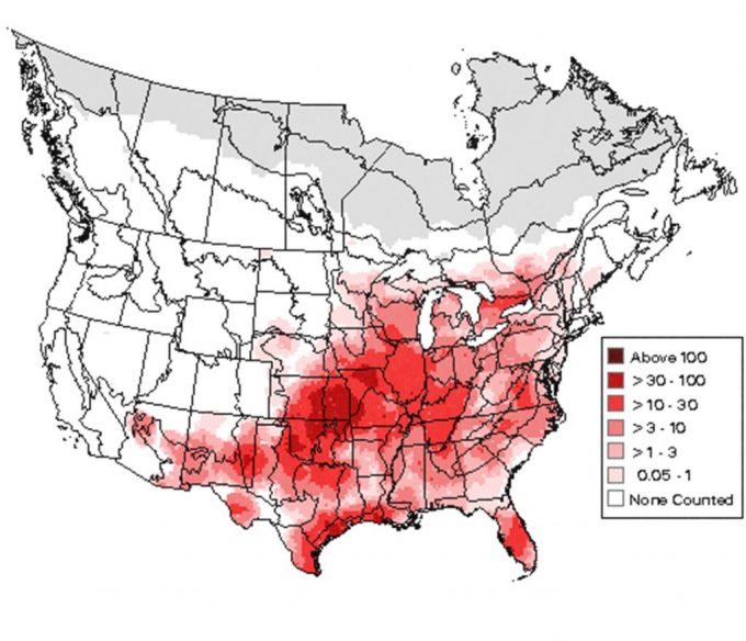
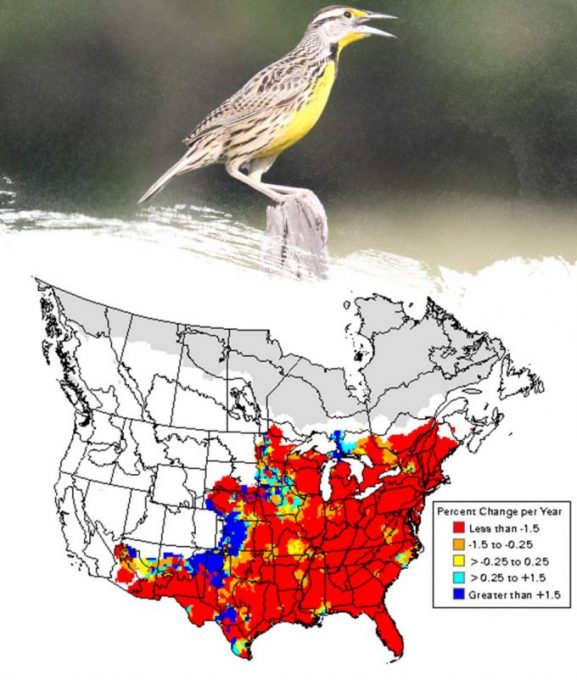
For instance, BBS data can be used to produce continental-scale maps of relative abundance. When viewed at continental or regional scales, these maps provide a reasonable indication of the relative abundances of species that are well sampled by the BBS (Figure 2.2). Analyzing population change on survey routes is probably the most effective use of BBS data, but these data do not provide an explanation for the causes of population trends. Population trend data have been used, however, to associate population declines with environmental effects such as habitat loss and fragmentation (Askins 1993; Boulinier et al. 1998b, 2001; Donovan and Flather 2002). To evaluate population changes over time, BBS indices from individual routes are combined to obtain regional and continental estimates of trends. Few species, however, have consistent trends across their entire ranges, so spatial patterns in population trends are of particular interest to scientists and managers attempting to identify “hot spots” of regional declines. Route-specific trends can be smoothed to produce trend maps that allow for the identification of regions of increase and decline (Figure 2.3).
Although trends at the species level will always be a basic use of BBS data analyses, combining species into groups with similar life-history traits, known as guilds, provides additional insight into patterns of population trends (Askins 1993, Sauer et al. 1996, Hines et al. 1999). The concept of grouping species based on certain life history characteristics (e.g., breeding habitat, migratory behavior, etc.) can be useful for identifying widespread environmental effects since individual species often differ widely in their response to environmental change. Consistent trends within an entire guild may be indicative of overall changes in an environmental resource (e.g., declining forest birds due to the loss of forests to development).
Environmental Monitoring and Assessment Program (EMAP)
National monitoring programs all share the common challenge of developing a monitoring framework that can scientifically determine and track the condition of a natural resource distributed over thousands of kilometers. Sometimes this need to monitor a natural resource is a legal mandate for a federal or state agency. As an example, under the Clean Water Act the Environmental Protection Agency (EPA) has statutory responsibilities to monitor and assess inland surface waters and estuaries. To achieve this goal, the Environmental Monitoring and Assessment Program (EMAP) was created to develop the science needed for a statistical monitoring framework to determine the condition, and to detect trends in condition, both at the level of individual States as well as for all the nation’s aquatic ecosystems (McDonald et al. 2002). Given its legal responsibility and need to produce legally defensible results, EMAP emphasizes a sampling design guided by both statistical and scientific objectives.
What is the goal of the monitoring?
The primary goal of EMAP is clear and was determined legislatively: to develop a sampling design that provides an unbiased, representative monitoring of an aquatic resource with a known level of confidence. The necessarily general nature of the objective informed a number of other steps in designing the monitoring program and outlined several key challenges. The need to be applicable across the landscape mandated that EMAP’s sampling design rely on a multi-scaled approach of collecting samples with State-based partners and aggregating those local data into broader state, regional, and national assessments. This approach of “scaling up” data from various locales requires EMAP’s research goals to include (1) establishing the statistical variability of EMAP indicators when used in aquatic ecosystems in diverse ecological areas of the country, (2) establishing the sensitivity of these indicators to change and trend detection, and (3) developing indicators and designs that will allow the additional monitoring of high-priority aquatic resources (e.g., Great Rivers, wetlands). The key challenge in this monitoring strategy, and one that is shared with many other national assessments, is how to draw a representative sample from a small number of sites to provide an unbiased estimate of ecological condition over a larger geographic region.
Where and how to monitor?
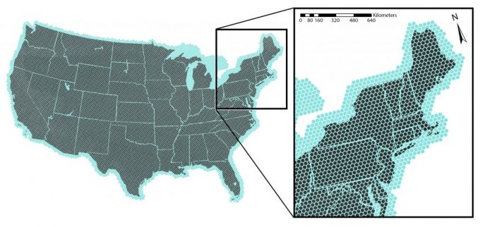
Choosing sites and methods that adequately addressed the key challenge was not easy. EMAP researchers have spent considerable time and effort in developing a probability-based sampling design to estimate the condition of an aquatic resource over large geographic areas. Probability-based sampling designs have a number of requirements including a clearly defined population, a process by which every element in the population has the opportunity to be sampled with a known probability, and a method by which that sampling can be conducted in a random fashion (Cochran 1977). As is the case with any monitoring project covering a larger geographic region, including the BBS described earlier, samples should be distributed throughout the study area to be maximally representative. EMAP’s design accomplishes this by taking samples at regular intervals from a random start (a systematic random design). To achieve this, EMAP uses hexagonal-shaped grids to add systematic sampling points across a study region (Figure 2.4) (White et al. 1991). The grid is positioned randomly on the map of the target area, and sample locations from within each hexagonal grid cell are selected randomly. Why is this necessary? In short, the use of a sampling grid ensures an unbiased spatial separation of randomly selected sampling units (systematic random sample). Also, the grid allows for the potential of dividing the entire target population into any number of sub-populations (or strata) of interest. Subsequent random sampling within these strata allows statistical inferences to be made about each sub-population. As an example, stratified sampling is often used in a regional stream survey to enhance sampling effort in a watershed of special interest so that its condition can be compared with the larger regional area.
What to monitor?
Once the sampling design was established, the next question to address was a familiar one: what exactly is to be measured? Like BEST’s efforts of monitoring environmental pollutants, an adequate response consisted of more than simply electing one indicator; there are many definitions of an “aquatic resource” that all have unique characteristics. At the coarsest level, EMAP addressed this by dividing aquatic resources into different water body or system types, such as lakes, streams, estuaries and wetlands. Subsequently, they use a second level of strata, ecoregions, to capture regional differences in water bodies. The lowest level of strata in the EMAP design distinguishes among different “habitat types” within an aquatic resource in a specific geographic region. For example, portions of estuaries with mud-silt substrate will have much different ecological characteristics than portions of estuaries with sandy substrates. It is within this lowest stratum that sampling and monitoring is conducted.
EMAP’s sampling design takes one of two very different routes depending on whether the aquatic ecosystem to be sampled is discrete or extensive (McDonald et al. 2002). A discrete aquatic system consists of distinct natural units, such as lakes. Population inferences for a discrete resource are based on numbers of sampling units that possess a measured property (e.g., 10% of the lakes are acidic). For discrete resources, EMAP often uses an intensification of the sampling grid. In some cases where the sampling units are a large enough area, the grid can be used directly by selecting those units in which one or more grid points fall (e.g., estuaries in a state). With this method, the probability that a unit gets into the sample (its inclusion probability) is proportional to the unit’s area (e.g., larger lakes have a higher probability of being sampled). The inferences linking sampling data to the entire population is then in terms of area. Alternatively, a unit of a discrete resource can be treated as a point in space. For example, the center point of lakes could be used. This method of sampling is appropriate for inference in terms of numbers of units in a particular condition (e.g., 7% of Northeastern lakes are chronically acidic).
Extensive resources, on the other hand, extend over large regions in a more or less continuous and connected fashion (e.g., rivers), and do not have distinct natural units. In these cases, population inferences are based on the length or area of the resource. The nature of the ecosystem determines the particular sampling technique that is used. EMAP uses area sampling for extensive systems such as rivers or point sampling for discrete systems like estuaries. In area sampling, the extensive resource is broken up into disjoint pieces, much like a jigsaw puzzle, and sample selection is from a random selection of these pieces. The sampling values that are obtained are then used to characterize or represent the entire resource. To avoid any sampling bias, points are located at random within the extensive resource.
Only once sites and appropriate sampling techniques are selected, can an indicator of ecological condition of the aquatic system be chosen and sampled. Effective aquatic ecological indicators are central to determining the condition of aquatic resources, and EMAP has identified a number of ecological indicators (see McDonald et al. 2002 for a full list). In general, EMAP focuses on combining biological indicators that are able to be sampled through analysis of the fish, benthic macroinvertebrate, and plant communities. EMAP also makes extensive use of an index of biotic integrity (IBI, a multi-metric biological indicator) (Karr 1981) to evaluate the overall fish assemblage, which provides a measure of biotic condition.
Nongovernmental Organizations and Initiatives
Monitoring the Illegal Killing of Elephants (MIKE)
Between 1970 and 1989, half of Africa’s elephants, over 700,000 individuals, were killed due to a surging international ivory trade (Douglas-Hamilton 1989, Blake et al. 2007). This decline prompted the Convention on the International Trade in Endangered Species of Wild Flora and Fauna (CITES) to list African elephants on Appendix I of the convention, banning the trade of tusks in international markets. Despite its protected status, the optimal approach to African elephant management and conservation remains a topic of great debate (Blake et al. 2007). In response to the need for better data regarding the status and trends of African Elephants (Figure 2.5), Monitoring the Illegal Killing of Elephants (MIKE) was initiated in 1997. The overall goal of MIKE is to provide the information needed for governments and agencies to make appropriate management and enforcement decisions, and to build institutional capacity for the long-term management of elephant populations. The MIKE program is funded by a diversity of agencies and NGOs including the Wildlife Conservation Society, United States Fish and Wildlife Service, the European Union, and the World Wildlife Fund.
What is the goal of the monitoring program?
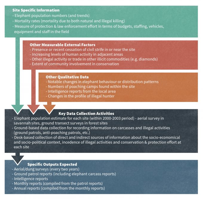
MIKE has three specific program objectives including to: 1) measure the levels and trends in the illegal hunting of elephants, 2) determine changes in these trends, and 3) determine the factors associated with these trends. Once again, the clarity of the objectives is central in developing other aspects of the monitoring program. In the case of MIKE, the breadth of the goals meant that a suite of factors needed to be investigated, including habitat type, elephant population levels, human conflicts, adjacent land uses, human access, water availability, tourism activities, civil strife, and development activities. The monitoring objectives of the program also emphasized a need for standardized methodologies, representative sampling, and collecting data on population trends and the spatial patterns of illegal killing (Figure 2.6). The nature of the objectives even clarified what the main benefit of this comprehensive monitoring scheme would be: an increased knowledge base of elephant numbers and movements, a better understanding of the threats to their survival, and an increased general knowledge of other species and their habitats.
Where and how to monitor?
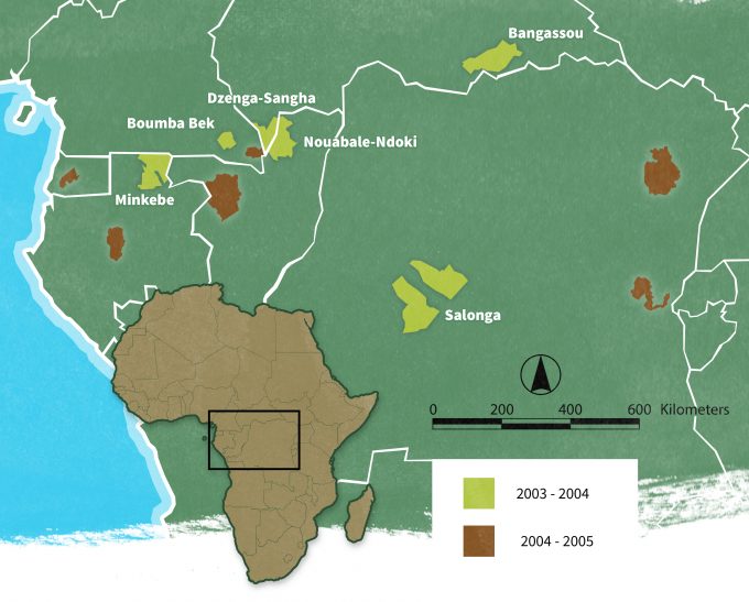
Given the remote location of many of the habitats and populations of interest (Figure 2.7), site selection was of paramount importance for collecting representative and unbiased data. A minimum of 45 sites in 27 states were initially selected in Africa and 15 sites in 11 states in Asia. The methods of site selection were based on a number of variables chosen to make the sites a representative sample, including habitat types, elephant population size, protection status of sites, poaching history, incidence of civil strife, and level of law enforcement. Statistical analysis and modeling have also been used to select sites based on geographical, environmental and socio-economic characteristics.
What to monitor?
In central Africa from 2003-04, Blake et al. (2007) used this approach to implement the first systematic, stratified, and un-biased survey of elephant populations within each MIKE site. The primary data source they elected to use were dung counts based on along line-transects. In addition to the standardized transects, they undertook reconnaissance surveys to provide supplementary information on the incidence of poaching and other human impacts. At each survey site, an attempt was made to sample elephant abundance across a gradient of human impact. Stratification of each site was based on elephant sign encounter rate generated during MIKE pilot studies or on expected levels of human impact as a proxy for elephant abundance. Sample effort was designed to meet a target precision of 25% (coefficient of variation) of the elephant dung density estimate. Density estimates of forest elephants in MIKE survey sites were obtained via systematic line-transect distance sampling that used dung counts as an indicator of elephant occurrence. Advanced data analysis (using distance sampling) provided robust estimates of dung density, relative elephant density, and spatial distributions within each site (Figure 2.8).
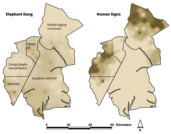
The decision to record a diversity of variables allowed researchers to conduct analyses that addressed all of the MIKE objectives and provided other valuable insights. Blake et al. (2007) found that human activities were a major determinant of the distribution of elephants even within highly isolated national parks. In almost all cases the relative elephant abundance interpolated from transect data was the mirror image of human disturbance, and elephant abundance was consistently highest farthest from human settlement (Figure 2.8). They estimated that, despite international attention and conservation status, forest elephants in central Africa’s national parks are losing range at an alarming rate. Twenty-two poached (confirmed) elephant carcasses were found from 4,478 km of reconnaissance surveys walked during the inventory period. The combined inventory, distribution, and reconnaissance data showed little doubt that forest elephants are under imminent threat from poaching and range restriction. This innovative monitoring scheme and analysis demonstrated that even with an international ban of the trade in ivory in place, forest elephant range and numbers are in serious decline.
Learning from Citizen-Based Monitoring
Volunteer-based monitoring efforts have a long history in the United States and throughout the world. For example, Audubon’s Christmas Bird Count (CBC) has been a volunteer-based annual survey of winter bird distributions throughout the United States dating back to the early 1900’s. Although biological surveys based on volunteer effort have a rich history, they are now being increasingly used for monitoring long-term and large-scale changes in animal and plant populations. The combination of current demand for broad-scale, long-term ecological data and an explosion of volunteer-based efforts has resulted in a fairly well-informed movement in which scientists have made great strides in increasing the scientific rigor of monitoring programs that involve citizens. This movement has become so popular in recent years that many of these programs and initiatives are falling under the global label of citizen science.
What is the goal of the monitoring program?
Although citizen science takes many forms and has many objectives (see Cornell Lab of Ornithology’s citizen science programs http://www.birds.cornell.edu/ ), atlas surveys are a globally common example and are widely implemented for many species and taxa. Atlases consist of volunteers documenting the distribution (and often breeding status) of species within a survey grid covering an entire region of interest (Donald and Fuller 1998, Bibby et al. 2000). The goal of many atlas surveys focuses on documenting and monitoring temporal and spatial shifts in species distributions over long time periods (Donald and Fuller 1998). One such example of a regional atlas is the New York State Breeding Bird Atlas (Andrle and Carroll 1988, McGowan and Corwin 2008). This project is sponsored by the New York State Ornithological Association and the Department of Environmental Conservation in cooperation with the New York Cooperative Fish and Wildlife Research Unit at Cornell University, Cornell University Department of Natural Resources, and the Cornell Laboratory of Ornithology. The New York State Breeding Bird Atlas (BBA) is a comprehensive, statewide survey with the specific objective of documenting the distribution of all breeding birds in New York. As with all the preceding monitoring programs, stating the program objective informs and drives other aspects of the monitoring program. For instance, its breadth indicates that substantial planning is needed to collect occurrence data for multiple species over a wide range of habitats and develop a protocol that can be easily followed and adhered to by voluntary participants. Time is an essential component of any monitoring program and atlases are often unique among other monitoring initiatives due to scope of their sampling. In the case of the New York State BBA, the surveys were conducted in two time periods: the first atlas project ran from 1980 to 1985 (Andrle and Carroll 1988) while New York’s second atlas covered 2000 to 2005 (McGowan and Corwin 2008). Broad-scaled distributional surveys, such as atlases, are obviously an attempt to monitor long-term range changes that are beyond the scope of most monitoring programs.
Where and how to monitor?
Given that it was necessary to account for the entire state to meet the objective of the BBA, researchers first had to determine how to make the scale manageable. For the New York State BBA, both surveys used a grid of 5,332 5- x 5-km blocks that covered the entirety of New York State (125,384 km2); representing one of the largest and finest resolution atlas data sets in the world (Gibbons et al. 2007). The state was stratified into ten regions and one or two regional coordinators in each area were responsible for recruiting volunteers in each atlas effort and overseeing coverage of the blocks in their region. Once this system was prepared, efforts were needed to ensure that the volunteers reported quality data despite monitoring independently from one another in different locations. To do this, the researchers assigned atlas surveyors to one or more blocks and instructed them to spend at least eight hours in the block, visiting each habitat represented, and recording data on at least 76 bird species. This “76 species” threshold was treated as a standard of “adequately surveyed” based on experience from previous atlases (Smith 1982). Measures such as these are integral to monitoring programs with multiple observers responsible for sampling different sites and species. Without some form of controlling and documenting variation in sampling effort, the data would be vulnerable to a number of biases.
What to monitor?
The objective of the BBA required that volunteers would survey their atlas block(s) and record every bird species encountered and the observed breeding activity ranging from possible breeding (e.g., singing male in appropriate habitat type), probable breeding (e.g., pair observed in breeding habitat), and confirmed breeding (e.g., nest found). Although the BBA did not provide a definitive statement concerning the absence of a breeding record for a species not listed in a block, absence was interpreted by researchers to mean that species could not be found given adequate effort and observer ability, or that the species occurs in low enough densities to escape detection. In addition, atlasers were asked to submit data on effort including the total number of hours spent surveying and the number of observers. Mandating that volunteers record a variety of data, including data on sampling efforts further reduced the possibility of biases (or at least allowed researchers to account for variation in effort during analyses).
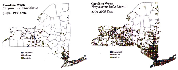
One final important lesson that can be drawn from programs such as the BBA is that researchers must be transparent about the appropriate significance and uses of the data they generate. Whether or not atlases can be used as an effective tool for monitoring animal populations relates to the relationship between changes in regional occupancy (as measured by atlas surveys) and changes in local abundance (Gaston et al. 2000). In macroecology, this relationship is synonymous with the abundance-occupancy rule which predicts that changes in regional occupancy will accurately reflect changes in local abundance. Relatively few studies have addressed the relationship between abundance and occupancy using atlas data, but those that have generally support the use of atlas data for monitoring large-scale population dynamics (Böhning-Gaese 1997, Van Turnhout et al. 2007, Zuckerberg et al. 2009). Once this information and relationship is made explicit, atlas data can be correctly used to make a number of observations and assessments. In the New York State BBA, with its two survey periods, researchers and managers can analyze the changes in regional distribution for over 250 bird species. Bird species demonstrated a wide variation in distributional changes from widespread increases (Figure 2.9) to startling range contractions (McGowan and Corwin 2008). Approximately half of all of the bird species in New York demonstrated significant changes in their distribution between the two atlases. Of those with significant changes, 55 percent increased in their distribution. As a group, woodland birds demonstrated a significant increase in their average distribution between the two atlas periods while grassland birds showed the only significant decrease (Zuckerberg et al. 2009). Scrub-successional, wetland, and urban species showed no significant change in their distribution between the two atlas periods (McGowan and Corwin 2008, Zuckerberg et al. 2009). Within migratory groups, there were significant increases in the overall distribution of permanent residents and short-distance migrants while Neotropical migrants showed no significant change. These trends suggest that certain regional factors of environmental change, such as reforestation or climate change, may be affecting entire groups of species.
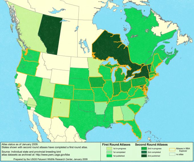
Atlases offer an excellent opportunity for monitoring changes in large-scale and long-term population dynamics. Furthermore, the quality of their data will almost certainly increase as future advances in monitoring are applied to atlas implementation and analysis. For instance, improvements in occupancy estimation and modeling will undoubtedly be applied to projects such as the BBA to account for the varying detection probabilities of different species and there are likely to be significant improvements in training models for participants to decrease observer bias even more (MacKenzie 2005, MacKenzie 2006). In addition, repeat atlases for several regions of the United States will be available in the near future (Figure 2.10). These databases will be critical for monitoring changes in species’ distributions in response to relatively broad-scale environmental drivers such as regional climate change.
Summary
Despite their varied interests, funding sources, and target species/communities, all of these monitoring programs share many of the same components and obstacles. Issues such as clearly defined monitoring goals and objectives, where, how, and what to sample are common aspects of many monitoring programs and will be discussed at length throughout this book. Despite the challenges presented to them, these programs represent how careful planning, committed individuals, and thoughtful sampling design and analysis can help answer critical questions and thereby further conservation goals for a variety of types of organizations. Whether it is predicting the effects of environmental contamination, estimating avian declines across an entire country or monitoring elephant populations in remote African forests, these programs serve as encouraging reminders of the power and effectiveness of monitoring information for guiding conservation decision-making.
References
Alpizar-Jara, R., J.D. Nichols, J.E. Hines, J.R. Sauer, K.H. Pollock, and C.S. Rosenberry. 2004. The relationship between species detection probability and local extinction probability. Oecologia 141:652-660.
Andrle, R.F., and J.R. Carroll. 1988. The atlas of breeding birds in New York State. Cornell University Press, Ithaca, New York.
Askins, R.A. 1993. Population trends in grassland, shrubland, and forest birds in eastern North America. Current Ornithology 11:1-34.
Barker, R.J., J.R. Sauer, and W.A. Link. 1993. Optimal allocation of point-count sampling effort. Auk 110:752-758.
Bibby, C. J., N. D. Burgess, D. A. Hill, and S. Mustoe. 2000. Bird census techniques. 2nd edition. Academic Press, San Diego, California.
Blake, S., S. Strindberg, P. Boudjan, C. Makombo, I. Bila-Isia, O. Ilambu, F. Grossmann, L. Bene-Bene, B. de Semboli, V. Mbenzo, D. S’hwa, R. Bayogo, L. Williamson, M. Fay, J. Hart, and F. Maisels. 2007. Forest elephant crisis in the Congo Basin. Plos Biology 5:945-953.
Böhning-Gaese, K. 1997. Determinants of avian species richness at different spatial scales. Journal of Biogeography 24:49-60.
Boulinier, T., J.D. Nichols, J.E. Hines, J.R. Sauer, C.H. Flather, and K.H. Pollock. 1998a. Higher temporal variability of forest breeding bird communities in fragmented landscapes. Proceedings of the National Academy of Sciences of the United States of America 95:7497-7501.
Boulinier, T., J.D. Nichols, J.E. Hines, J.R. Sauer, C.H. Flather, and K.H. Pollock. 2001. Forest fragmentation and bird community dynamics: Inference at regional scales. Ecology 82:1159-1169.
Boulinier, T., J.D. Nichols, J.R. Sauer, J.E. Hines, and K.H. Pollock. 1998b. Estimating species richness: The importance of heterogeneity in species detectability. Ecology 79:1018-1028.
Cam, E., J.D. Nichols, J.R. Sauer, J.E. Hines, and C.H. Flather. 2000. Relative species richness and community completeness: Birds and urbanization in the Mid-Atlantic states. Ecological Applications 10:1196-1210.
Cochran, W. G. 1977. Sampling Techniques. 3rd edition. John Wiley & Sons, New York.
Donald, P.F., and R.J. Fuller. 1998. Ornithological atlas: a review of uses and limitations. Bird Study 45:129-145.
Donovan, T.M., and C.H. Flather. 2002. Relationships among North American songbird trends, habitat fragmentation, and landscape occupancy. Ecological Applications 12:364-374.
Douglas-Hamilton, I. 1989. Overview of status and trends of the African elephant.in S. Cobb, editor. The ivory trade and the future of the African elephant: Prepared for the Seventh CITES Conference of the Parties, Lausanne, October 1989. Ivory Trade Review Group, Oxford, United Kingdom.
Flather, C.H., and J.R. Sauer. 1996. Using landscape ecology to test hypotheses about large-scale abundance patterns in migratory birds. Ecology 77:28-35.
Gaston, K.J., T.M. Blackburn, J.J.D. Greenwood, R.D. Gregory, R.M. Quinn, and J.H. Lawton. 2000. Abundance-occupancy relationships. Journal of Applied Ecology 37:39-59.
Gibbons, D.W., P.F. Donald, H.-G. Bauer, L. Fornasari, and I.K. Dawson. 2007. Mapping avian distributions: the evolution of bird atlases. Bird Study 54:324-334.
Harris, T. 1991. Death in the marsh. Island Press, Washington, D.C.
Hines, J.E., T. Boulinier, J.D. Nichols, J.R. Sauer, and K.H. Pollock. 1999. COMDYN: software to study the dynamics of animal communities using a capture-recapture approach. Bird Study 46:209-217.
Johnson, R.E., T.C. Carver, and E.H. Dustman. 1967. Residues in fish, wildlife, and estuaries. Pesticides Monitoring Journal 1:7-13.
Karr, J.R. 1981. Assessment of biotic integrity using fish communities. Fisheries 6:21-27.
Kendall, W.L., B.G. Peterjohn, and J.R. Sauer. 1996. First-time observer effects in the North American Breeding Bird Survey. Auk 113:823-829.
La Sorte, F.A., and M.L. McKinney. 2007. Compositional changes over space and time along an occurence-abundance continuum: anthropogenic homogenization of the North American avifauna. Journal of Biogeography 34:2159-2167.
Link, W.A., and J.R. Sauer. 1997a. Estimation of population trajectories from count data. Biometrics 53:488-497.
Link, W.A., and J.R. Sauer. 1997b. New approaches to the analysis of population trends in land birds: Comment. Ecology 78:2632-2634.
Link, W.A., and J.R. Sauer. 1998. Estimating population change from count data: Application to the North American Breeding Bird Survey. Ecological Applications 8:258-268.
Link, W.A., and J.R. Sauer. 2007. Seasonal components of avian population change: joint analysis of two large-scale monitoring programs. Ecology 88:49-55.
MacKenzie, D.I. 2005. What are the issues with presence-absence data for wildlife managers? Journal of Wildlife Management 69:849-860.
MacKenzie, D I. 2006. Occupancy estimation and modeling : inferring patterns and dynamics of species. Elsevier, Burlington, MA.
Marshal, E. 1986. Selenium in western wildlife refuges. Science 231:111–112.
McDonald, M. E., S. Paulsen, R. Blair, J. Dlugosz, S. Hale, S. Hedtke, D. Heggem, L. Jackson, K. B. Jones, B. Levinson, A. Olsen, J. Stoddard, K. Summers, and G. Veith. 2002. Research Strategy: Environmental Monitoring and Assessment.
McGowan, K.J., and K. Corwin. 2008. The Second Atlas of Breeding Birds in New York State. Cornell University Press, Ithaca, New York.
Pollock, K.H., J.D. Nichols, T.R. Simons, G.L. Farnsworth, L.L. Bailey, and J.R. Sauer. 2002. Large scale wildlife monitoring studies: statistical methods for design and analysis. Environmetrics 13:105-119.
Sauer, J.R., J.E. Fallon, and R. Johnson. 2003. Use of North American Breeding Bird Survey data to estimate population change for bird conservation regions. Journal of Wildlife Management 67:372-389.
Sauer, J.R., W.A. Link, J.D. Nichols, and J.A. Royle. 2005. Using the North American Breeding Bird Survey as a tool for conservation: A critique of BART et al. (2004). Journal of Wildlife Management 69:1321-1326.
Sauer, J.R., W.A. Link, and J.A. Royle. 2004. Estimating population trends with a linear model: Technical comments. Condor 106:435-440.
Sauer, J.R., G.W. Pendleton, and B.G. Peterjohn. 1996. Evaluating causes of population change in North American insectivorous songbirds. Conservation Biology 10:465-478.
Sauer, J.R., B.G. Peterjohn, and W.A. Link. 1994. Observer differences in the North-American Breeding Bird Survey. Auk 111:50-62.
Smith, C.R. 1982. What constitues adequate coverage? New York State Breeding Bird Atlas Newsletter 5:6.
Spellerberg, I.F. 2005. Monitoring ecological change. 2nd edition. Cambridge University Press, Cambridge, UK.
Thogmartin, W.E., F.P. Howe, F.C. James, D.H. Johnson, E.T. Reed, J.R. Sauer, and F.R. Thompson. 2006. A review of the population estimation approach of the North American landbird conservation plan. Auk 123:892-904.
U.S. Geological Survey. 2007. Strategic Plan for the North American Breeding Bird Survey: 2006-2010: U.S. Geological Survey Circular 1307, 19 pp.
Van Turnhout, C.A.M., R.P.B. Foppen, R.S.E.W. Lueven, H. Siepel, and H. Esselink. 2007. Scale-dependent homogenization: Changes in breeding bird diversity in the Netherlands over a 25-year period. Biological Conservation 134:505-516.
White, D., A.J. Kimmerling, and W.S. Overton. 1991. Cartographic and geometric components of a global sampling design for environmental monitoring. Cartography and Geographic Information Systems 19:5-22.
Zuckerberg, B., W.F. Porter, and K. Corwin. 2009. The consistency and stability of abundance-occupancy relationships in large-scale population dynamics. Journal of Animal Ecology 78:172-181.
