14 Changing the Monitoring Approach

Despite the best efforts at designing a monitoring plan, it is nearly inevitable that changes will be made to the monitoring strategy sooner or later. Indeed, if monitoring data are used as intended in an adaptive management framework, the information gained should be used to refine the monitoring approach and improve the quality and utility of the data that are collected (Vora 1997). Marsh and Trenham (2008) summarized 311 surveys sent to individuals involved with monitoring programs in North America and Europe and estimated that 37% of the programs made changes to the overall design of the monitoring program at least once and that data collection techniques changed in 34% of these programs. Adding novel variables to measure is also often incorporated into monitoring programs as information reveals new, perhaps more highly valued, patterns and processes. Another change, dropping variables, oftentimes must accompany these additions simply due to increased costs associated with measuring more things. And clearly the vagaries of budget cycles can cause variables to be dropped for one or more monitoring cycles and then re-added if budgets improve. But changes to monitoring programs can result in some or all of the data collected to date being incompatible with data collected after a change is made. Increased precision in data collection is always a goal, but if data are collected with two levels of precision over two periods of time, then pooling the data becomes problematic. Similarly, changing the locations or periodicity of sampling can lead to discontinuities in the data; this makes analyses more challenging. Given these concerns, changing a monitoring program should not be done lightly and is a process that necessitates as much preparation as establishing the initial monitoring plan. Despite this, there is remarkably little information available to inform monitoring program managers when they consider changing approaches within their program.

General Precautions to Changing Methodology

In light of the paucity of references, it is important to carefully consider those that do exist. For instance, Shapiro and Swain (1983) noticed the enormous impact a change in methodology had on data analysis in a monitoring program involving water quality in Lake Michigan. Indeed, the apparent decline in silica concentration between 1926 and 1962 was an artifact of having changed methods and not a result of increased phosphorus loads as had been reported prior to their work (Shapiro and Swain 1983). Strayer et al. (1986) described this classic example of the dangers associated with changing methodology during a monitoring program further and used the experience to suggest several general precautions to take when changing methodology in the middle of a long-term monitoring program.

1. Calibrate the new methods against the old methods for a sufficient period of time.
2. Maintain a permanent detained record of all protocols used
3. Archive reference samples of materials collected in the field where appropriate. Voucher specimens, soil or water samples, and similar materials should be safely and securely archived for future reference. Consider collecting hair, feather, scale or other tissues form animals for future DNA analyses.
4. Change methods as infrequently as possible.

When to Make a Change

Although alterations should certainly be minimized, there will be instances in which a change will make monitoring more valuable than maintaining the original design. There will also be instances in which changes are unavoidable due to data deficiencies or stakeholder desires. Changes made to the design, in the variables measured, in the sampling techniques or locations, in the precision of the samples, or in the frequency of sampling are all potentially helpful. Yet they also all have the potential to detract from a monitoring program in unique and powerful ways. Determining when or if to change your program, therefore, can be a difficult task. So, when should a monitoring program be changed? The following examples describe some potentially appropriate or necessary scenarios, but it is important to keep in mind that all potential changes merit careful consideration

Changing the Design

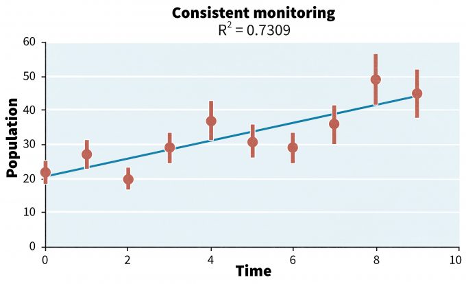
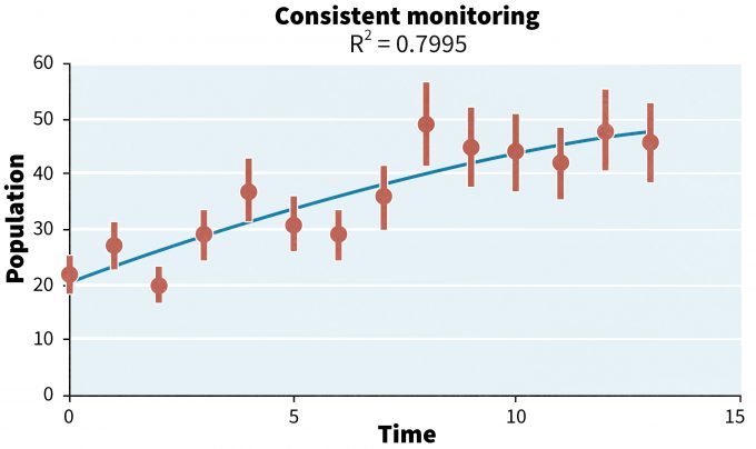
The initial stages of a monitoring program result in a series of data points and associated confidence intervals that describe a trend over space or time. Once that trend is established, new questions often emerge or, as new techniques are developed that are more useful or precise, a change in the design might be warranted. For example, the pattern observed in Figure 14.1 represents a positive trend, but the precision of the estimates may come into question since the data in time periods 4, 5 and 6 reflect a plateau. This realization leads to a number of questions that would undermine the monitoring program if left unanswered: Is this plateau real or a function of imprecise data collection? Are other variables such as fecundity or survival better indicators of population response than simply population sizes? If a change in design can answer these questions and make data more useful, and staying the course cannot, managers and stakeholders may decide that it is time to make some changes even after only 5 years of data collection.

Changing the Variables that are Measured

Changing the variables measured may be considered for a number of reasons, but should be undertaken prudently because it can set a monitoring program back to the very beginning. One legitimate reason to change the variables, however, is a failure to meet the goals and objectives of the project or a sudden change in the desires of stakeholders. If goals and objectives are not being met by the data being collected, it is obvious that changes must be made. In such a case, data collected to date may still be very useful to decision makers. These data may help to inform decisions made regarding how the changes ought to be made (altering variables measured or intensity of sampling). Using data in post-hoc power analyses has also become quite popular when trying to understand why a significant trend was not observed, but the logic behind post-hoc power analysis has been considered inherently flawed by some authors because the point of power analysis is to ensure during the design phase of a project that if a trend is real then there is an ‘x’ percent chance that it can be detected (Hoenig and Heisey 2001). Data analyses that include confidence intervals on parameter estimates are particularly useful in understanding the deficiencies of the underlying data and informing decisions regarding what changes to make and how and when to make them. This is especially true when failure to reject a null hypothesis (e.g., unable to detect a trend) could be erroneous and jeopardize a population.

Once the data have been analyzed, and the uncertainty associated with parameter estimates is understood, then all stakeholders can be informed about the changes that could be made in the monitoring plan to better meet their goals and objectives and then ensure that they are involved in the decision-making process.

Returning to our example, (Figure 14.1), positive trends may be encouraging, but if the data are needed to describe the degree of recovery and potential delisting under the Endangered Species Act, then stakeholders likely would suggest that population parameters describing reproductive rates and survival rates may also need to be measured. In this case, an entirely new monitoring program may be added to the populations monitoring program or monitoring of demographic parameters may simply be added to the existing protocol. Alternatively, sampling animal abundance may even be dropped and replaced with estimates of animal demographics, and hence truncating the continued understanding of population trends. The extent and form the changes take will depend on budgets, logistics, and stakeholder support and will ultimately be determined by assessing the potential costs associated with change relative to the perceived benefits and opinions of the stakeholders and funders.

Changing the Sampling Techniques

As new techniques become available that provide more precise or more accurate estimates of animal numbers, habitat availability or demographic parameters, the tendency is to use the new methods in place of less precise or less accurate methods used to date. This can also be a very appropriate scenario in which to change a monitoring program, but should be undertaken with a controlled approach if at all possible.

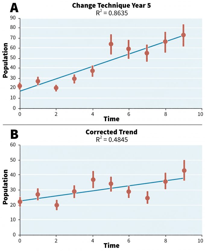
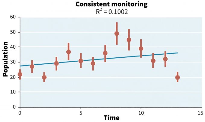
What does this entail? Consider the pattern in Figure 14.2a. Changing techniques in year 5 results in a higher R² and an abrupt change in population estimates. Because changes over time are confounded with changes in techniques, we cannot be sure if the observed trend line is real or an artifact of the changes in techniques.

Using a more controlled approach by making the change to the new technique in year 5 but also continuing to use the old technique as well for years 5-9, however, has the potential to inform managers of the effect due to technique change (Sutherland 1996). This is especially true if a statistical relationship (regression) between the data collected using both techniques allows the managers to standardize the data points for years 0-4 (Figure 14.2b). Such an approach requires extrapolation to years where only one technique was used (not both), and such extrapolations are accompanied by confidence intervals that describe the uncertainty in the data.

This more controlled process has been taken by others and led to informed, helpful changes to already established monitoring programs (Buckland et al. 2005). When the Common Bird Census (CBC) in the United Kingdom were established, the proposed techniques were state of the art. Over time however the methods were questioned and increasingly viewed as obsolete. Despite these concerns, the flawed methods were still used due to a fear of that any change would undermine the value of the long time series (Buckland et al. 2005). Eventually it became obvious that changing the methods had the potential to rectify the problem of misleading and unhelpful data and was therefore necessary. The British Trust for Ornithology decided to replace the CBC with a Breeding Bird Survey (BBS) in the United Kingdom that was similar to the North American BBS. Yet they also decided to conduct both approaches simultaneously for several years to allow calibration of CBC data to BBS data to provide a bridge in understanding how the results from one technique was associated with another which then allowed them to move to the BBS approach (Buckland et al. 2005). Strayer (1986) also advised employing new and old techniques simultaneously for a calibration period when changing techniques.

Changing the Sampling Locations

Changing the sampling locations over time can introduce variability into the data that may make detections of patterns difficult or impossible and many practitioners would therefore be very hesitant to do so. Nonetheless, in several cases it may be required for monitoring to be meaningful. First, not changing sampling location in environments that change more rapidly than the populations that are being monitored will confound data so much that analysis may be impossible unless the location is changed. Consider sampling beach mice on coastal dune environments. If a grid of sample sites are established and animals are trapped and marked year after year, the trap stations may become submerged as the dune location shifts over time. Similar problems arise when sampling riparian systems. Moving the sampling locations is required in these instances. In order to reduce the variance introduced into the sample by continually changing locations, stratification of sampling sites based on topographic features or (if necessary) vegetation structure or composition can help to reduce variability. Nonetheless such stratification will not entirely compensate for increases in variability due to changing sampling locations. It is important to keep this in mind at the outset of a monitoring program designed to sample organisms in dynamic ecosystems. Unless the variability in samples due to changing locations is considered during experimental design, it is possible, and indeed likely, that the statistical power estimated from a pilot study that does not sample new places each year will be inadequate to detect patterns. The pilot study should explicitly consider the variability associated with changing sampling locations from year to year.

The second case in which the sampling location may warrant a change is due to a deficient or misleading pilot study and involves a one-time alteration. While organisms may behave according to certain trends over time or space, one can never be certain that the data from a pilot study embodies those trends. To be more specific, if the goal of a monitoring program is to collect data on a particular population of a particular organism, it is likely necessary to choose a sampling location that either constitutes or is embedded within the home range of that population. A pilot survey is therefore necessary to choose the location. Yet, as organisms are normally not physically restricted to their home range, it is possible that survey data from a pilot study could suggest a sampling location that is hardly ever frequented by the focal species. This may be particularly likely for wide-ranging species such as the white-lipped peccary. Given this species’ tendency to travel in herds of several hundred animals over an enormous area, the presence of individuals or of sign at one point in time, even if abundant, may not be a good indication of the frequency with which a location is used (Emmons and Feer 1997). If the sampling location chosen inhibits the collection of the desired population parameters, an alteration to the sampling location is necessary.

Changing the Precision of the Samples

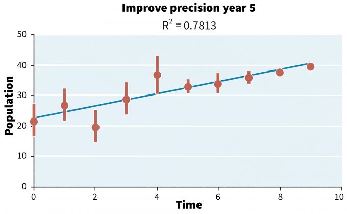
Despite having collected pilot data and designed a monitoring protocol to detect a given rate of change in a population, unexpected sources of variability may arise (human disturbances, climate, etc.) that reduce your ability to detect a trend. Increasing sample size or reducing sampling error can lead to more precise estimates as illustrated in Figure 14.3 after year 5. After making this change the fit of the line to the points is considerably tighter and the variance about the points is considerably less, leading to greater assurance that the population is indeed increasing. Such changes increase the R² somewhat (0.74 to 0.78) but the R² rose from 0.58 for the first 5 years to 0.99 during the second 5 years after improving precision.

But given the risks of altering a monitoring program, is it worth making a change just to increase precision? At what level is an increase in precision worth the risks of making a change? There is no simple answer to these questions; the program managers and stakeholders would need to decide if the added costs associated with increasing precision are worth the increased level of certainty associated with the trend estimates.

Changing the Frequency of Sampling

Given constraints on time, money and people, a decision might have to be made to reduce the level of effort associated with monitoring. Consider the trend in Figure 14.4 where the trend over the first 5 years was positive (R² = 0.58). In this case, program managers and stakeholders might agree that given the slope of the line there is little need to be concerned about this population, but that they want to continue some level of monitoring to ensure that the population does not begin to decline in the future. They may decide to reduce the frequency with which monitoring is conducted to every other year with the agreement that should there be more than 2 consecutive samples showing a decline that they would then revert back to annual sampling.

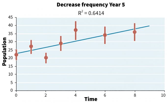
Such an approach should not be taken lightly, however. For instance, in our example, the reduced sampling did continue to demonstrate continual increases in abundance, but the R² associated with the trend declined. Such a decline in explanatory power may not be particularly important to the stakeholders so long as the population is increasing, but the level of certainty in that trend should also be valuable information to certain stakeholders and therefore carefully considered before making the change. It is also necessary to consider that high precision now may be important for the future. Should the population show declines over time, maintaining the sampling frequency and the high precision of the estimates now may facilitate future management decisions. Changes such as these come at a cost in certainty, money, and time and truly must be made prudently.

Logistical Issues With Altering Monitoring Programs

One other key component of prudently changing a monitoring program is that the program manager consider the logistical constraints associated with those changes. Training personnel in new techniques requires added time prior to the field sampling season. Where data standardization is necessary then collecting data using both the old and the new techniques adds considerable time and effort to field sampling. Changing locations may mean re-establishing sampling points and recording new GPS locations.

Changing variables that will be measured may require new equipment, additional travel, or different sampling periods. For example, sampling survival of post-fledging birds will require different techniques, sampling strategies, and sampling times than estimating abundance of adults from variable circular plot data. These new logistical constraints will need to be evaluated relative to the societal and scientific value of the monitoring program to determine if the making the changes is a tenable endeavor.

Economic Issuess With Altering Monitoring Programs

Changing monitoring programs in any way usually results in at least an initial expenditure of funds for equipment, travel, or training. It is thus important to address the economic questions of whether the change will result in increased costs, and if so, are the new data worth the increases in costs. This clearly must be done prior to making the change.

Keep in mind that a modest increase now will tend to compound itself over time, especially in the case of added per-diems or salaries for new staff, which must be iteratively increased to reflect cost of living trends, or added fuel consumption, which will almost certainly bring increasing costs over time due to rising fuel prices. A simple cost:benefit analysis is a useful way to estimate the marginal increases (or decreases) in costs associated with alternative changes in the monitoring program. The ultimate question that must be addressed is, “Where will you be getting the best information at the least cost and still stay within your budget”?

Terminating the Monitoring Program

The decision to terminate a monitoring program is probably the most difficult decision that a program manager can make. Obviously you end a program when you have answered the questions associated with your goals and objectives, correct? But how do you know when that is?

Consider the information in Figure 14.1. It seems quite obvious that the population is increasing. What if we extended the monitoring program another 4-5 years? Perhaps we would see the population approach an asymptote, which we would expect if a carrying capacity was reached (Figure 14.5). At this point, if the monitoring program was established to determine when and if a certain population target was attained, it would be logical to terminate the monitoring program; or if any monitoring was to be continued, it would be appropriate to only maintain it at a minimal level and a low cost.

Alternatively, if the data showed a different trend, such as a decline (Figure 14.6), it would be unwise to assume that the population was increasing or even remaining stable. The decline in population during the last 5 years could simply be due to chance, or to a population cycle, or to some biophysical factor leading to a true long-term decline. Unless comparable data had been collected on reference sites, we would not know if this pattern is likely a cyclic population or if a local event had occurred that would lead to a continued decline. In this case, key questions have not been answered, the goals and objectives of the monitoring program have not been attained, and there is a strong argument for the continuation of monitoring.

Summary

Changing a monitoring program is done frequently and has significant consequences with regards to the utility of the data, costs, and logistics. If the data that are collected and analyzed suggest that the goals and objectives are not being met adequately as determined by program management and stakeholders, then revisions in the protocol will be required. Adding or deleting variables, altering the frequency of data collecting, altering sample sizes or changing techniques to increase precision can all improve a monitoring program and help to meet goals and objectives more comprehensively. Yet all of these changes can also lead to changes in costs, in power to detect trends, or other patterns, thus any potential alteration to a monitoring program must be carefully considered.

References

Buckland S.T, A.E. Magurran, R.E Green, and R.M. Fewster. 2005. Monitoring change in biodiversity through composite indices. Philosophical Transactions of the Royal Society Biology. 360.

Emmons, L. and F. Feer. Neotropical rainforest mammals: a field guide. The University of Chicago Press, Chicago.

Hoenig, J.M., and D.M. Heisey. 2001. The abuse of power: The pervasive fallacy of power calculations for data analysis. The American Statistician 55(1): 19-24.

Marsh, D.M., and P.C. Trenham. 2008. Current trends in plant and animal population monitoring. Conservation Biology 22:647–655

Shapiro, J., and E.B. Swain. 1983. Lessons from the silica decline in Lake Michigan. Science 221 (4609): 457–459.

Strayer, D., J.S. Glitzenstein, C.G. Jones, J. Kolas, G. Likens, M.J. McDonnell, G.G. Parker, and S.T.A. Pickett. 1986. Long-term ecological studies: an illustrated account of their design, operation, and importance to ecology. Occasional Paper 2. Institute for Ecosystem Studies, Millbrook, New York.

Sutherland, W.J. 1996 Ecological census techniques. Cambridge University Press.

Vora, R.S. 1997. Developing programs to monitor ecosystem health and effectiveness of management practices on Lakes States National Forests, USA. Biological Conservation 80:289-302.