13 Uses of the Data: Synthesis, Risk Assessment and Decision Making

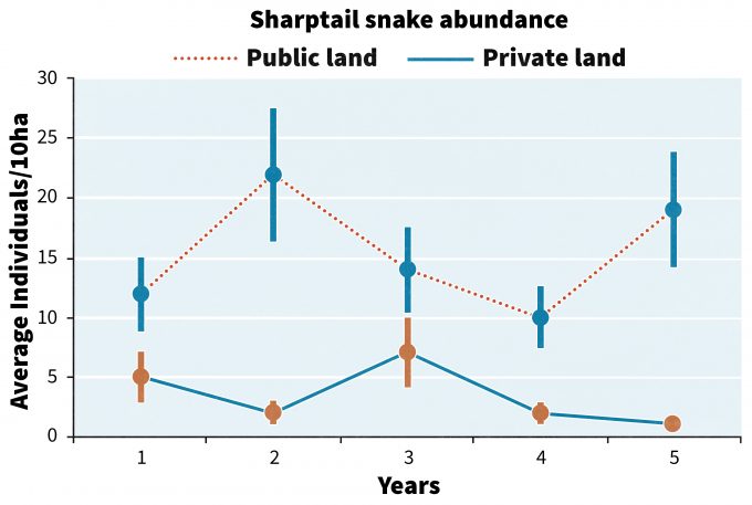
Imagine the following scenario. You have just spent nearly $500,000 over the past five years collecting information on changes in the abundance of sharptail snakes in the foothills of the Willamette Valley in Oregon. Data were collected from 30 randomly selected sites on public land managed to restore Oregon oak savannahs, and on another 30 sites on private lands that are grazed. The data are presented in figure 13.1.

So given this information, what do you do? Continue to monitor? Use the information to make changes? What are the risks of changing vs. continuing on with the status quo? Can these data be integrated with monitoring data from other programs to create a broader picture of the state of Oregon’s ecosystems? We will follow this example through a few key steps in interpreting monitoring data and see how decisions might be made.

Thresholds and Trigger Points

Clearly there are a number of issues that must be considered not only by managers but also by stakeholders before making any changes. One approach is to agree with stakeholders at the outset of the monitoring program that if a particular threshold or trigger point is reached then alternative management actions are to be implemented. Block et al. (2001) differentiated between trigger points that initiate a change to enact recovery, and thresholds, that indicate success in a recovery action. In the case of figure 13.1, a trigger point may be recording < 5 snakes/10ha for two or more consecutive years. If such a trigger point is reached, it could be agreed with stakeholders beforehand that a series of steps would be taken by the responsible agency to restore habitat for the species. Or in the case of endangered species, the decision may be made to capture individuals and initiate a captive breeding program. But in our hypothetical case after 5 years, sharptail snake detections meet the trigger point at year 5, so at that point the public management agency biologists may begin meeting with private landowners to explore the following options to restore habitat for the species:

• Provide landowner assistance on habitat restoration
• Provide incentives to landowners to alter grazing and other land use practices.
• Explore purchase of a conservation easement that allows public biologists to manage land
• Explore purchase of key properties and begin habitat restoration

Any one of the above options may be acceptable to one landowner but not to another. As these or other options are implemented then continued monitoring can allow detection of the point at which a threshold of recovery, say >10 snakes/10 ha for >2 years, is surpassed and maintained. Monitoring a control area to understand changes in abundance on public conservation land will provide a point of comparison to help ensure that the patterns seen on private lands using the above approaches are more likely caused by management actions than to other extraneous effects. For instance, if the abundance on both the public and private lands declined over time despite changes in management practices on the private lands then declines are more likely due to factors unassociated with management such as changes in climate or disease.

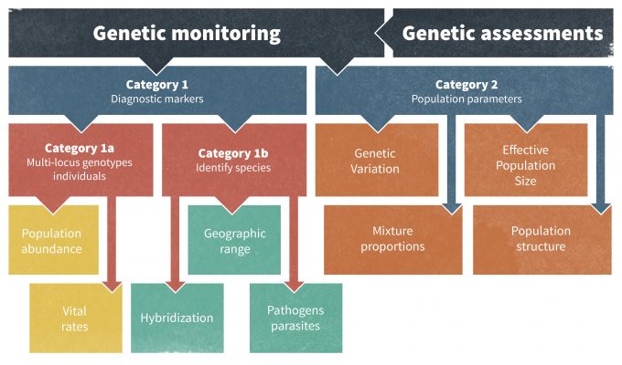
One possible problem with the identification of thresholds is that they are the result of social negotiation and although they may be based in biology they may also simply represent an agreed upon, socially acceptable point by managers and stakeholders. Thresholds based on biology may represent population density, probability of occurrence, a change in reproduction or survival (or lambda), genetic heterozygosity, or other population parameters, but the threshold(s) are set jointly by biologists and stakeholders. Use of genetic markers to assess changes in effective population size and other aspects of population ecology have become increasingly popular (Schwartz et al. 2007).  Schwartz et al. (2007) described two categories of monitoring using genetic markers: Category I which can identify individuals, populations, and species; and Category II which monitors population genetic parameters allowing insights into demographic processes and ‘retrospective monitoring’ to better understand historical changes (Figure 13.2). Thresholds may also, however, constitute more of a reflection of society’s tolerance of or desires for a particular species. For instance, the threshold for the number of cougars in a residential area of California may be the level that the public can tolerate rather than what is most significant in terms of the population dynamics of the species.

Forecasting Trends

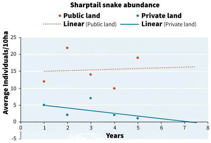
With 5 years of data, trends can begin to emerge from the data (Figure 13.3) that provide information to guide management actions. In our hypothetical example, trends on public lands are rather stable, whereas those on private lands are declining. If we forecast the trend from private lands into the future we can see that in 2.5 years the x intercept for the trend will reach 0. The degree of precision in estimating the x intercept decreases dramatically as forecasts are extended further into the future, so forecasting attempts should be viewed as one tool to guide decision making. It is not clear if the x intercept will be reached in 1 year, 2.5 years or 10 years, or at all, but the trend line does raise concerns about the long term viability of the species on private lands and may initiate a more rapid response than if the trend line had an x intercept of 15 years. Dunn (2002) used an approach similar to this and categorized over 200 bird species into conservation alert categories.

But these are simply linear trends and the variability associated with trends, especially for rare species, is often very high. Indeed, the power associated with detecting a significant trend is often very low with rare species, thus statistical trend lines must be interpreted cautiously to avoid making an error of concluding that no trend exists when it actually is in a decline. This is especially problematic when populations have already reached very low levels and the probability of detecting an additional decline is very low (Staples et al. 2005). In these cases it may be more useful to employ risk assessments based on population viability analyses (PVA, Morris et al. 2002, Lande et al. 1993). If the data collected in monitoring can be used to aid in parameterizing a PVA model, then at least relative changes in future population abundance or time-to-extinction can be estimated (Dennis et al. 1991, Morris and Doak 2002). Staples et al. (2002) proposed a viable population monitoring approach in which yearly risk predictions are used as the monitoring indicator. Staples et al. (2002) defined ‘risk’ as “the probability of population abundance declining below a lower threshold within a given time frame.” Predicting that risk will increase over time could constitute a trigger point and prompt alternative management actions.

Predicting Patterns Over Space and Time

Clearly managers would like to know where on a landscape species are likely to occur so that management actions can be taken to increase, or decrease populations or at least have minimal effects on desired species. Monitoring occurrence of organisms across a landscape can provide information in the spatial distribution of individuals within populations and can provide a better understanding of metapopulation structure and connectivity among subpopulations. If information on reproduction and survival are also included in the monitoring effort then additional information on the value of subpopulations as sources or sinks can also be gained. And if this information is collected over time then information on the probabilities of subpopulations becoming locally extinct in patches and subsequent recolonization can also be understood through long-term monitoring.

Although this baseline information on the distribution and fitness of organisms over a planning area is valuable information for understanding the impacts of managing landscapes, issues such as land use and climate change make the information even more valuable. In the face of such changes, the risk of species loss from an area, or even overall extinction, depends on the rate at which a species can adapt to changing conditions. Monitoring information can provide evidence to more fully understand both the rates of change in the biophysical environment and the associated fitness of organisms. In the following sections we use monitoring in the context of climate change as an example to show how environmental stressors can influence how managers act to attempt to conserve biodiversity, but also the difficulties of confronting such comprehensive ecological changes.

If we continue to pump CO₂ into the atmosphere at current rates, then approximately 20-30% of plant and animal species assessed by the IPCC (2007) are likely to be at increased risk of extinction as global average temperature increases by 1.5 to 2.5°C or more. Hence understanding certain aspects of the environment and species responses through monitoring is key to providing opportunities for species to adapt to or recover from climate change. But climate change is probably one of the more difficult environmental stressors to respond to even with good monitoring data because it is global – the opportunity for comparisons between sites affected by climate change and those unaffected by change are rare if they exist at all. Indeed, we are not usually given the opportunity to use BACI or comparative mensurative approaches when designing a monitoring plan affecting regional or global stressors, so we must rather rely on associations over time. To be more specific, effect may be inferred from these data only with care since other factors associated with change may have a greater or lesser effect in any observed trends. Nonetheless there are a number of potential factors that are often assessed when trying to understand effects of global changes like climate change on loss of biodiversity.

Geographic Range Changes

If global average temperature increases exceed 1.5 to 2.5°C, then major changes in ecosystem structure and function, species’ ecological interactions and shifts in species’ geographical ranges, are anticipated, with predominantly negative consequences

for biodiversity (IPCC 2007). Because geographic ranges of species are often dictated by climatic conditions (or by topographic barriers) that influence physiological responses, changes in geographic ranges of species are frequently predicted using bioclimate envelopes (Pearson and Dawson 2003), and observed changes are used as an early indicator of a species’ response and ability to adapt to climate change. But bioclimate envelopes are coming under scrutiny and being questioned because biotic interactions, evolutionary change, and dispersal ability also influence the ability or inability of a species to respond to changes in its environment (Pearson and Dawson 2003). One can easily imagine how the impacts of climate change on subpopulations could be exacerbated by land use change that leads to their isolation; indeed these subpopulations would become more vulnerable to local extinction through inability to disperse, infectious disease, or competition with invasive species as their habitat changes in response to climate change.

Zuckerberg et al. (2009) used the New York State Breeding Bird Atlas surveyed in 1980–1985 and 2000–2005 to test predictions that changes in bird distribution are related to climate change. They found that 129 bird species showed an average northward range shift in their mean latitude of 3.6 km (Zuckerberg et al. 2009) and that the southern range boundaries of some bird species moved northward by 11.4 km. Clearly these monitoring programs can provide evidence for associations between climate change and changes in geographic ranges, yet other factors should not be ruled out. Human population density has changed over that time as have land use patterns and both could have had similar effects on the geographic range of certain species. Nonetheless the compelling fact is that all of the 129 species that they examined showed a northward shift in distribution, thus in this case, the data suggest that the driving influence is something more global and consistent in its impact. Similar efforts at using monitoring information over time can elucidate changes for less mobile species such as plants, invertebrates and amphibians (Walther et al. 2002).

Home Range Sizes

Resource availability is related to home range size for many species. Climate change quite likely will influence the dispersion or concentration of available food and cover resources for many species (McNab 1963). Therefore, monitoring home range sizes also constitutes a method for assessing ecological effects of climate change on some species.

Documenting the sizes of home ranges can be costly and estimates can suffer from low precision for a number of reasons (Borger et al. 2006). Estimating the effect size that could be detected (a power analysis would help determine this, Zielinski and Stauffer 1996), can allow a better understanding of the actual risks of losing species.

Some effects are obvious in the higher latitudes. As sea ice is lost and shifts in its locations, polar bears must extend their foraging bouts into new locations (Derocher et al. 2004). If the energy that they expend in foraging exceeds the energy they gain from catching prey then they will die. With polar bears and other species, expanding home range size can be an early warning indicator of decreased or dispersed resources availability and an indication that the species may be facing imminent population declines. Changes in home range sizes hence can be an important aspect of risk analysis. If home range sizes are expanding then risk of population decline is greater than if they are stable to contracting and changes in hope range size may be detectable prior to a decline in abundance.

Phenological Changes

Another early warning sign of impending impacts of climate change on populations are changes in the phenological patterns of plants and animals. Indeed, events such as the arrival at breeding or wintering sites from migrations, onset of flowering or other reproductive activities, leaf-out, or leaf fall function as indicators because they tend to be influenced at least in part by temperature (Parmesan 2007). Phenological studies have been conducted for years (e.g., Menzel 2000), but not on the global scale necessary for monitoring global climate change. Schwartz (1994) provided a discussion on the detection of large-scale changes using phenological information. He commented on how past efforts at recording phenological patterns have often been done at small scales, and then suggested that by integrating ground-based data collection with remotely-sensed data, local patterns can be appropriately scaled to ecoregions, continents and ideally the globe, allowing larger scale patterns to be inferred. White et al. (2005) proposed a global framework for monitoring phenological responses to climate change using remotely sensed data. If White et al.’s (2005) approach can be implemented effectively then the physical mechanisms responsible for observed patterns can be used to assess the effectiveness of global-scale models in predicting changes in phenological events (Schwartz 1994).

Habitat Structure and Composition

For some purposes, simply understanding changes in the availability of habitat for a species may be sufficient to infer likely changes in a species potential abundance or distribution. The devil is in the details however. For many species, knowledge of abundance and spatial arrangement of fine scale habitat elements such as large trees, snags, logs, or shrubs is important. But gathering this knowledge on a large scale can pose problems; satellite imagery will not detect many of these features. LIDAR or other remotely sensed data, however, can often provide information at a fine enough scale to detect habitat components (Hyde et al. 2006). LIDAR in particular can provide information on the fine-scale vertical complexity of a forest including canopy heights and canopy biomass (Hyde et al. 2006). For those species associated with vegetative layers in forests, remotely-sensed data may be useful. For species associated with dead wood or other habitat elements that are not detectable using remote techniques then combining remotely sensed data with ground plot data becomes the only logical approach. These fine scale habitat elements can be imputed to pixels from known locations of ground plots using nearest-neighbor techniques (Ohmann and Gregory 2002).

Synthesis of Monitoring Data

Monitoring data can be integrated with other information on terrain, climate, disturbance probabilities, land use, land ownership, and infrastructure to paint a generalized integrated picture of the state of a landscape. These approaches allow managers to monitor not only the individual pieces of the landscape but also the integrated whole over time. For instance, changes in the structure and composition of forest stands in Oregon with and without certain silvicultural practices can be incorporated into maps of forest age classes and habitat types (Spies et al. 2007). These can then be linked to models of forest growth and development (many of which are based on continuous forest inventory monitoring plots), and to transition probabilities associated with land management decisions, allowing projections of possible future conditions for planning purposes and to better understand the implications of possible changes in land use policy (Spies et al. 2007). Other approaches have not explicitly used vegetation growth models but have developed scenarios of past conditions, current conditions and likely alternative future conditions of landscapes (Baker et al. 2004). It is important to stress that these approaches not only use monitoring information to parameterize many of the spatial and temporal projections, but also to improve our understanding of possible future conditions. Indeed, it is the ability to use data to create models that allow projections of conditions into the future based on interacting stressors such as climate change (IPCC 2007) and land use planning (Kaiser et al. 1995). These model projections not only raise the potential for developing ‘what-if’ scenarios to compare alternative policies, but they can identify key parameters that should be monitored into the future to help stakeholders understand if the results of a policy change are being realized as projected. There are so many interacting assumptions that enter into these complex landscape projections that without monitoring data, the projections are at best a likely future condition and at worst an artifact of an incorrect assumption. Some practitioners also attempt to integrate ecological monitoring data with economic, social, and institutional information in order to create bodies of data that function as sustainability indicators. This has often been done for agricultural systems and for communities in developing countries but is expanding to include other regions, such as highly developed urban environments (Olewiler 2006, Van Cauwenbergh et al. 2007). Not all of these initiatives necessarily include the monitoring of populations or habitat, but many do. For instance, to assess the sustainability of the terrestrial resource use of communities in tropical ecosystems, several researchers have integrated wildlife monitoring and the mapping of hunting kill-sites with data regarding the use of other terrestrial resources, access to new technologies, and changing local land uses (Koster 2008, Parry et al. 2009). In the Sustainability Assessment of Farming and the Environment (SAFE) framework for developing a set of variables that indicate the sustainability of agro-ecosystems, variables that measure the retention of biodiversity and the “functional quality of habitats” are considered an integral component of the monitoring framework (Van Cauwenbergh et al. 2007). While monitoring wildlife and habitat is not explicitly discussed within the framework guidelines, it would be difficult to make such assessments without doing so. It is also important to realize that the concept of “sustainability indicators” and previous attempts at deriving them has its share of critics. Scerri and James (2009), for instance, discuss how many practitioners reduce the complex concept of sustainability and the generation of sustainability indicators that is likely context specific to a very technical, quantitative task.

PVA models typically compare the estimated risk of a species or population going extinct among several management alternatives. PVA models are notoriously data-hungry requiring age- or stage-specific estimates of survival, reproduction and movements with associated ranges of variability for each parameter estimate (Beissenger and Westphal 1998, Reed et al. 2002). As with projections of landscape models, monitoring aspects of PVA projections allow not only an assessment of risk associated with not achieving an expected result but also highlight the weaknesses in the model assumptions. Monitoring programs that inform the validity of assumptions can provide the opportunity for developing more reliable model structures and resulting projections. Deciding which assumptions or parameters to monitor based on a model structure can be problematic, especially with large complex models such as the two described above. Identification of variable to monitor may be based on subjective assessment of the reliability of the underlying data or through more structured sensitivity analyses that identify variables that have an over-riding influence on the model results (McCarthy et al. 1995, Fieldings and Bell 1997). Quite often the least reliable parameters in these models are those that are the most difficult to measure. This can create a dilemma for a program manager developing a monitoring program since these data may be the most important to lead to a decrease in uncertainty in future predictions but they may also be the most expensive to acquire. Hence a benefit:cost assessment will need to be made with stakeholders to develop a priority list of variables.

Despite the ability to develop more reliable estimates of key variables from monitoring data, projections into the future are always faced with the inability to predict unknown threshold events that would not have been foreseen at the outset. For instance, barred owl invasions into spotted owl habitat were not seriously considered as much of a threat as habitat loss when early PVAs for spotted owls were developed (Peterson and Robins 2003). And even when models can consider new or confounding variables, the inter-relationships among the variables can give rise to new states or processes that could not be foreseen.

Climates have always changed on this earth but the rate of change likely to be seen in the next century could be unprecedented. Changes in vegetative community structure and inter-specific relationships are likely to change, but their ability to adapt to changing climatic conditions is in question. Williams and Jackson (2007) provided an overview of no-analog plant communities associated with historic “novel” climates and future novel climates which are likely to be warmer than any present. Ecological models such as forest dynamics models and PVA models are at least partially parameterized from relatively recently collected data, so they may not accurately predict responses to novel climates (Williams and Jackson 2007). The uncertainty raised by the potential development of no-analog conditions must be explicitly considered during risk analyses.

Risk Analysis

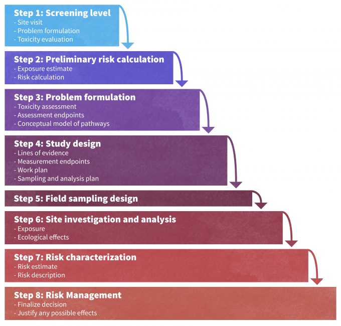
Risk analyses have been formally developed with regards to direct and indirect effects of pollutants on wildlife species. The Environmental Protection Agency defines Ecological Risk Assessment (ERA) as, “an evaluation of the potential adverse effects that human activities have on the living organisms that make up ecosystems. The risk assessment process provides a way to develop, organize and present scientific information so that it is relevant to environmental decisions. When conducted for a particular place such as a watershed, the ERA process can be used to identify vulnerable and valued resources, prioritize data collection activity, and link human activities to their potential effects. ERA results provide a basis for comparing different management options, enabling decision-makers and the public to make better informed decisions about the management of ecological resources”(http://epa.gov/superfund/programs/nrd/era.htm). The steps used by the EPA are outlined in Figure 13.4, and could be adapted for use in other situations where risks from other environmental stressors or disturbances may be of key importance to managers (e.g., fires, land use, floods, etc.). For instance, Hull and Swanson (2006) provided a stepwise process for assessing risk to wildlife species from exposure to pollutants. Similar approaches have been proposed to assess risk to loss of biodiversity. Kerns and Ager (2007) described risk assessment as a procedure to assess threats and understand uncertainty by “…providing: (1) an estimation of the likelihood and severity of species, population, or habitat loss or gain, (2) a better understanding of the potential tradeoffs associated with management activities, and (3) tangible socioeconomic integration.” They proposed a quantitative and probabilistic risk assessment to provide a bridge between planning and policy that includes stakeholder involvement (Kerns and Ager 2007). Such formal approaches are needed within ecological planning processes if both managers and stakeholders are to understand uncertainty, and the costs associated with the risks of not achieving the intended results.

Decision Making

From a logical standpoint, decisions should be made using a sequence of steps: characterize the problem or question, identify a full range of alternatives and determine

criteria for selecting one, collect information about each option and rate it on the criteria, then make the final decision based on the rating (Lach and Duncan 2007). But Klein (2001) found that only 5% of all decisions are made using such a logical approach. Individuals often make their decisions using intuition and mental simulations (quickly relating the outcome of a decision to some experience) (Lach and Duncan 2007). Groups may make decisions differently and groups are better able to make better decisions on complex problems than individuals (Lach and Duncan 2007). People with different world views structure the world around them in different ways and in so doing bring a different perspective to a group decision. Ensuring that a range of world views is represented in a group can be particularly useful when trying to reach a balanced decision on a complex issue, though discussions needed to reach that decision may necessarily become protracted.

Summary

Considerable time and money are invested in many monitoring programs so not only must the design of these programs be scientifically and statistically rigorous, it must be clear to the managers and stakeholders how the information will be used to make decisions. During the design phase, trigger points or thresholds should be identified to ensure that managers know when changes in management approaches should be considered. In many circumstances it is easy for managers to simply wait for more information without taking an action, not realizing that waiting places greater risk on achievement of desired outcomes. Using monitoring data as the basis for forecasting trends over space and time can allow managers to understand the implications of waiting too long before taking remedial actions. Factors such as changes in climatic characteristics, phenology, geographic ranges, and home range sizes of some species can be particularly informative in the face of global changes to climate for which the only reference condition is the past. Using monitoring information as a means of parameterizing models of landscape or climate change allows projections over space and times of more complex conditions. Such integrative approaches further allow comparisons among alternative management strategies or policies and can be an important component of a risk analysis, a formalized approach to identifying uncertainties and assessing direct and indirect effects of stresses on organisms and ecosystems. The results of monitoring, modeling and risk analysis are then used to make decisions by individuals or by groups. Although we typically assume that decisions are made in a logical manner many decisions are made based on intuition or as the result of group discussions among people with various world views.

References

Baker, J.P., D.W. Hulse, S.V. Gregory, D. White, J. Van Sickle, P.A. Berger, D. Dole, and N.H. Schumaker. 2004. Alternative futures for the Willamette river basin. Ecological Applications 14:313–324.

Beissinger, S.R. and M.I.Westphal. 1998. On the use of demographic models of population viability in endangered species management. Journal of Wildlife Management 62: 821-841.

Block, W.M., A.B. Franklin, J.P. Ward Jr., J.L. Ganey, and G.C. White. 2001. Design and implementation of monitoring studies to elucidate the success of ecological restoration on wildlife. Restoration Ecology 9:293–303.

Borger, L., N. Franconi, F. Ferretti, F. Meschi, G. De Michele, A. Gantz, A. Manica, S. Lovari, and T. Coulson. 2006. Effects of sampling regime on the mean and variance of home range size estimates. Journal of Animal Ecology 75:1393–1405.

Dennis, B., P.L. Munholland, and J.M. Scott. 1991. Estimation of growth and extinction parameters for endangered species. Ecological Monographs 61:115–143.

Derocher, A., Lunn, N.J., Stirling, I. 2004. Polar bears in a warming climate. Integrative Comparative Biology 44:163–176.

Dunn, E.H., 2002. Using decline in bird populations to identify needs for conservation action. Conservation Biology 16:1632–1637.

Fieldings, A.H., and J.F. Bell. 1997. A review of methods for the assessment of prediction errors in conservation presence: absence models. Environmental Conservation 24: 38–49.

Hull R.N., and S. Swanson. 2006. Sequential analysis of lines of evidence—An advanced weight-of-evidence approach for ecological risk assessment. Integrated Environmental Assessment and Management 2:302–311.

Hyde, P., R. Dubayah, W. Walker, J.B. Blair, M. Hofton and C. Hunsaker. 2006. Mapping forest structure for wildlife habitat analysis using multi-sensor (LiDAR, SAR/InSAR, ETM+, Quickbird) synergy. Remote Sensing of Environment 102: 63-73

IPCC. 2007. Climate change 2007: synthesis report. Contribution of working groups I, II and III to the fourth assessment report of the Intergovernmental Panel on Climate Change. IPCC, Geneva, Switzerland, 104 pp.

Kaiser, E., D. Godschalk, and F.S. Chapin. 1995. Urban land use planning. University of Illinois Press, Fourth Edition. Urbana, IL.

Kerns, B.K. and A. Ager. 2007. Risk assessment for biodiversity conservation planning in Pacific Northwest forests. Forest Ecology and Management 246: 38-44.

Klein, G. 2001. Understanding and supporting decision making: An interview with Gary Klein. Information Knowledge Systems Management 2(4):291–296.

Koster, J. 2008. The impact of hunting with dogs on wildlife harvests in the Bosawas Reserve, Nicaragua. Environmental Conservation 35(3):221-220.

Lach, D. and S. Duncan. 2007. How do we make decisions? Chapter 2, pages 12-20 in Johnson, K.N., S. Gordon, S. Duncan, D. Lach, B. McComb, and K. Reynolds. Conserving creatures of the forest: a guide to decision making and decision models for forest biodiversity. National Commission on Science for Sustainable Forestry Final report. NCSSF, Washington, DC.

Lande, R. 1993. Risks of population extinction from demographic and environmental stochasticity and random catastrophes. The American Naturalist 142:911–927.

McCarthy, M.A., M.A. Burgman, and S. Ferson. 1995. Sensitivity analysis for models of population viability. Biological Conservation 73:93-100.

McNab, B.K. 1963. Bioenergetics and the determination of home range size. The American Naturalist 97:133-141.

Menzel A. 2000. Trends in phenological phases in Europe between 1951 and 1996. International Journal of Biometeorology 44:76–81.

Morris, W.F., P.L. Bloch, B.R. Hudgens, L.C. Moyle, and J.R. Stinchcombe. 2002. Population viability analysis in endangered species recovery plans: past use and future improvements. Ecological Applications 12:708–712.

Morris, W.F., and D.F. Doak. 2002. Quantitative conservation biology: theory and practice of population viability analysis. Sinauer Associates, Sunderland, MA.

Ohmann, J.L. and Gregory, M.J., 2002. Predictive mapping of forest composition and structure with direct gradient analysis and nearest neighbor imputation in coastal Oregon, USA. Canadian Journal of Forest Research 32:725-741.

Olewiler, N. 2006. Environmental sustainability for urban areas: the role of natural capital indicators. Cities 23(3):184-195.

Parmesan, C. 2007. Influences of species, latitudes and methodologies on estimates of phenological respons­es to global warming. Global Change Biology 13:1860–1872.

Parry, L., J. Barlow, and C.A. Peres. 2009. Allocation of hunting effort by Amazonian smallholders: Implications for conserving wildlife in mixed-use landscapes. Biological Conservation. 142:1777–1786

Pearson, R.G., and T.P. Dawson. 2003. Predicting the impacts of climate change on the distribution of species: are bioclimate envelope models useful? Global Ecology and Biogeography 12:361-371.

Peterson, A.T. and C.R. Robins. 2003. Using ecological-niche modeling to predict barred owl invasions with implications for spotted owl conservation. Conservation Biology 17:1161–1165.

Reed, J.M., L.S., Mills, J.B. Dunning, E.S. Menges, K.S.McKelvey, R. Frye, S.R. Beissinger, M.C. Anstett, and P. Miller. 2002. Emerging issues in population viability analysis. Conservation Biology 16: 7–19.

Scerri, A. and P. James. 2009. Communities of citizens and ‘indicators’ of sustainability. Community Development Journal. doi:10.1093/cdj/bsp013

Schwartz, M.D. 1994. Monitoring global change with phenology: The case of the spring green wave. International Journal of Biometeorolology 38:18–22.

Schwartz M.K., G. Luikart, and R.S. Waples. 2007. Genetic monitoring as a promising tool for conservation and management. Trends in Ecology & Evolution 22:25–33.

Spies, T.A., K.N. Johnson, K.M. Burnett, J.L. Ohmann, B.C. McComb, G.H. Reeves, P. Bettinger, J.D. Kline, and B. Garber-Yonts. 2007. Cumulative ecological and socioeconomic effects of forest policies in coastal Oregon. Ecological Applications 17:5–17.

Staples D.F., M.L. Taper, and B.B. Shepard. 2005. Risk-based viable population monitoring, Conservation. Biology 19:1908–1916.

Van Cauwenbergh, N., K. Biala, C. Bielders, V. Brouckert, L. Franchois, V. Garcia Cidad, M. Hermy, E. Mthij, B. Muys, J. Rejinders, X. Sauvenier, J. Valckx, M. Vancloster, B. Van der Veken, E. Wauters, and A. Peeters. 2007. SAFE—a hierarchical framework for assessing the sustainability of agricultural systems. Agriculture, Ecosystems and Environment 120:229–242.

Walther, G.-R., E. Post, P. Convey, A. Menzel, C. Parmesan, T.J C. Beebee, J.-M. Fromentin, O. Hoegh-Guldberg, and F. Bairlein, 2002. Ecological responses to recent climate change. Nature 416:389–395.

White, M.A., F. Hoffman, W.W. Hargrove, and R.R. Nemani. 2005. A global framework for monitoring phonological responses to climate change. Geophysical Research Letters 32:L04705.

Williams, J. W., and S. T. Jackson. 2007. Novel climates, no-analog communities and ecological surprises. Frontiers in Ecology and the Environment 5:475–482.

Zielinski, W.J., and H.B. Stauffer. 1996. Monitoring Martes populations in California: survey design and power analysis. Ecological Applications 6:1254–1267

Zuckerberg, B., A.M. Woods and W.F. Porter. 2009. Poleward shifts in breeding bird distributions in New York State. Global Change Biology 15:1-18