29 R Functions
While we could continue to cover R’s unique and powerful vector syntax, it’s time to have some fun and learn about functions. Functions in R are similar to their Python counterparts: they encapsulate a block of code, making it reusable as well as allowing us to consider the block in isolation of the rest of the program. As with functions in most languages, R functions consist of three main parts:
- The input (parameters given to the function).
- The code block that is to be executed using those parameters. In R, blocks are defined by a matching pair of curly brackets,
{and}. - The output of the function, called the return value. This may be optional if the function “does something” (like
print()) rather than “returns something.”
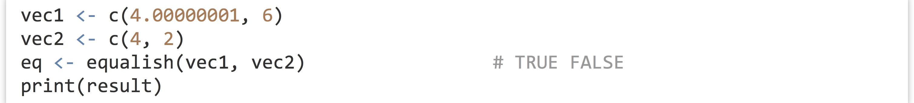
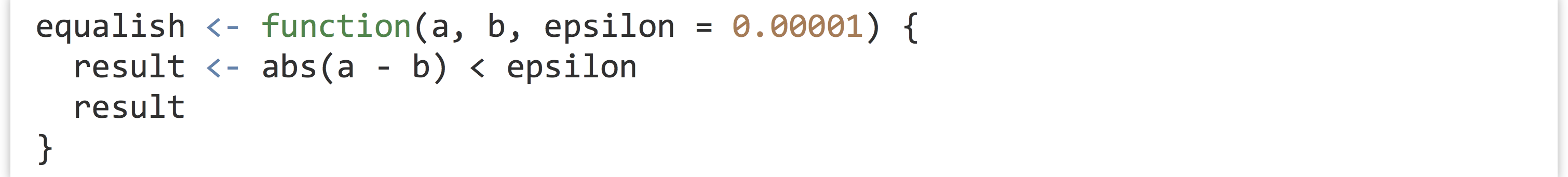
Let’s consider the problem of determining which elements of two numeric vectors, say vec1 and vec2, are close enough to equal to call them equal. As mentioned in chapter 27, “Variables and Data,” the standard way to check if all elements in two equal-length vectors are approximately pairwise-equal is to use isTRUE(all.equal(vec1, vec2)), which returns a single TRUE if this is the case and a single FALSE if not.
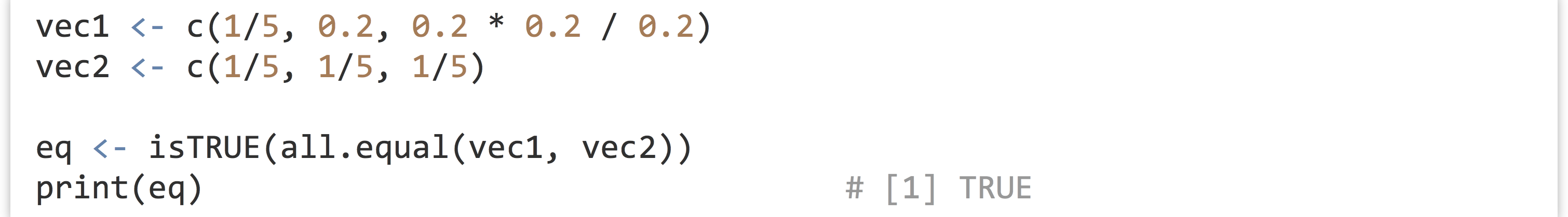
But perhaps we’d rather like a logical vector indicating which elements are approximately equal. The most straightforward way to do this is by comparing the absolute difference between the elements with some small epsilon value.
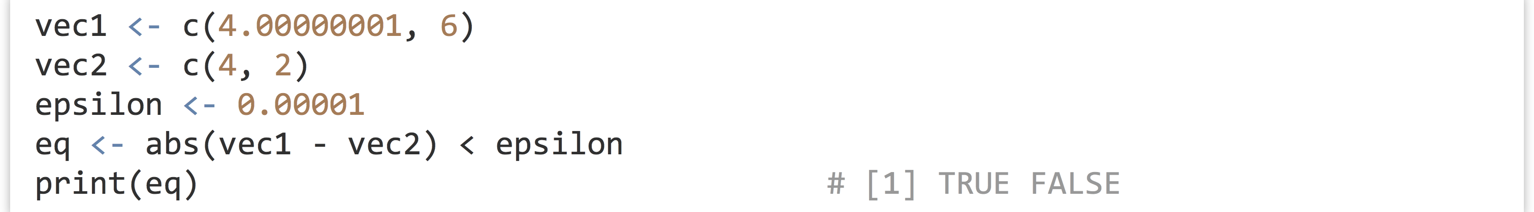
As a review of the last chapter, what is happening here is that the - operation is vectorized over the left- and right-hand sides, producing a vector (using vector recycling if one of the two were shorter, which not the case here; see chapter 28), as is the abs() function, which takes a vector and returns a vector of absolute values. Similarly, the < operator is vectorized, and because epsilon is a vector of length one, so it is compared to all elements of the result of abs(vec1 - vec2) using vector recycling, for the final result of a logical vector.
Because this sort of operation is something we might want to perform many times, we could write a function for it. In this case, we’ll call our function equalish(); here’s the R code for defining and running such a function.

There are many things to note here. First, when defining a function, we define the parameters it can take. Parameters in R functions have a position (a is at position 1, b is at position 2, and epsilon is at position 3) and a name (a, b, and epsilon). Some parameters may have a default value: the value they should have if unspecified otherwise, while other parameters may be required: the user of the function must specify them. Default values are assigned within the parameter list with = (not <- as in standard variable assignment).
The block that defines the operations performed by the function is enclosed in curly brackets, usually with the opening bracket on the same line as the function/parameter list definition, and the closing bracket on its own line. We’ve indented the lines that belong to the function block by two spaces (an R convention). Although not required, this is a good idea, as it makes code much more readable. The value that is returned by the function is specified with a call to a special return() function—functions can only return one value, though it might be something sophisticated like a vector or data frame.[1]
After a function has been defined, it can be called, as in eq <- equalish(vec1, vec2). The variable names associated with the data outside the function (in this case vec1 and vec2) needn’t match the parameter names inside the function (a and b). This is an important point to which we will return.
In the call above, we let the epsilon parameter take its default value of 0.00001. We could alternatively use a stricter comparison.

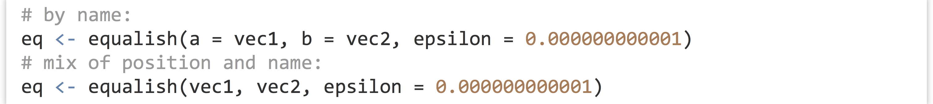
In R, arguments to functions may be specified by position (as in the example above), by name, or by a combination.
Many R functions take a few required parameters and many nonrequired parameters with reasonable defaults; this calling scheme allows us to specify the required parameters as well as only those nonrequired ones that we wish to change.
In general, you should specify parameters by position first (if you want to specify any by position), then by name. Although the following calls will work, they’re quite confusing.

We frequently use default parameters to specify named parameters in functions called within the function we’re defining. Here is an example of a function that computes the difference in means of two vectors; it takes an optional remove_NAs parameter that defaults to FALSE. If this is specified as TRUE, the na.rm parameter in the calls to mean() is set to TRUE as well in the computation.
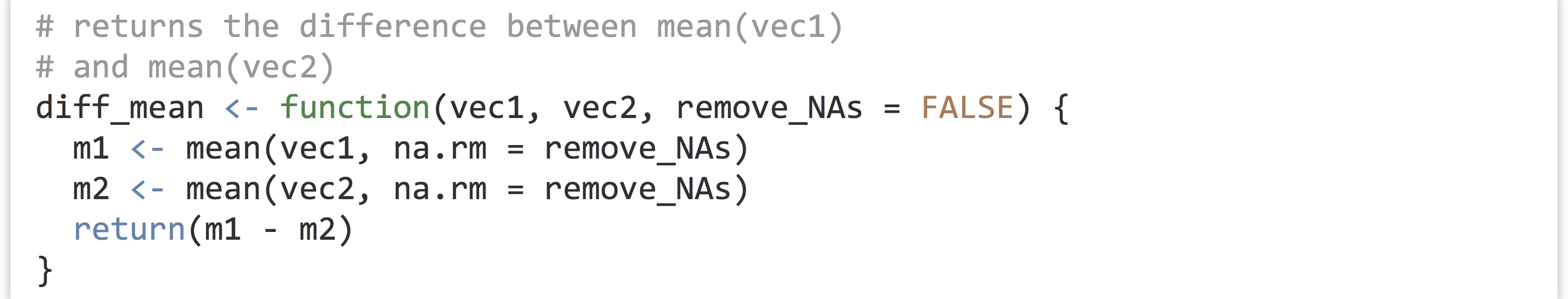
For continuity with other R functions, it might have made better sense to call the parameter na.rm; in this case, we would modify the computation lines to read like m1 <- mean(vec1, na.rm = na.rm). Although it may seem that the R interpreter would be confused by the duplicate variable names, the fact that the mean() parameter na.rm happens to have the same name as the variable being passed will cause no trouble.
Variables and Scope
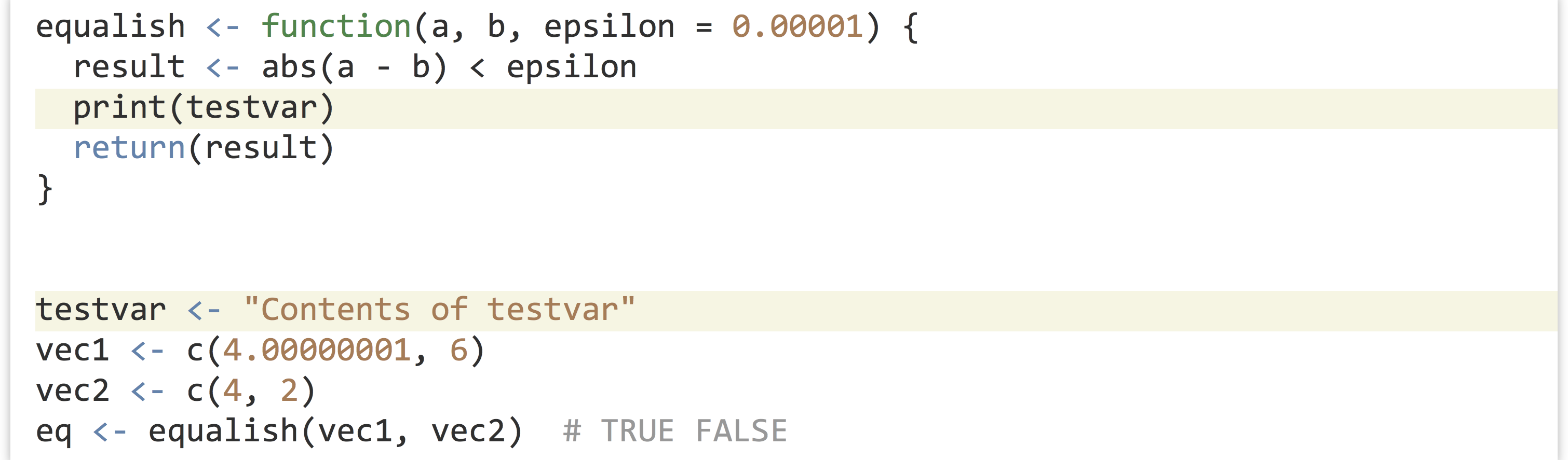
Let’s run a quick experiment. Inside our function, the variable result has been assigned with the line result <- abs(a - b) < epsilon. After we run the function, is it possible to access that variable by printing it?
Printing doesn’t work!

This variable doesn’t print because, as in most languages, variables assigned within functions have a scope local to that function block. (A variable’s scope is the context in which it can be accessed.) The same goes for the parameter variables—we would have no more success with print(a), print(b), or print(epsilon) outside of the function.
One of the best features of these local variables is that they are independent of any variables that might already exist. For example, the function creates a variable called result (which we now know is a local variable scoped to the function block). What if, outside of our function, we also had a result variable being used for an entirely different purpose? Would the function overwrite its contents?

True to the independence of the local result variable inside the function, the contents of the external result are not overwritten.

This feature of how variables work within functions might seem somewhat strange, but the upshot is important: functions can be fully encapsulated. If they are designed correctly, their usage cannot affect the code context in which they are used (the only way standard R functions can affect the “outside world” is to return some value). Functions that have this property and always return the same value given the same inputs (e.g., have no random component) are called “pure.” They can be treated as abstract black boxes and designed in isolation of the code that will use them, and the code that uses them can be designed without consideration of the internals of functions it calls. This type of design dramatically reduces the cognitive load for the programmer.
Now, let’s try the reverse experiment: if a variable is defined outside of the function (before it is called), can it be accessed from within the function block definition?
The lack of error in the output indicates that yes, the function block can access such external variables:

This means that it is possible to write functions that take no parameters and simply access the external variables they will need for computation.
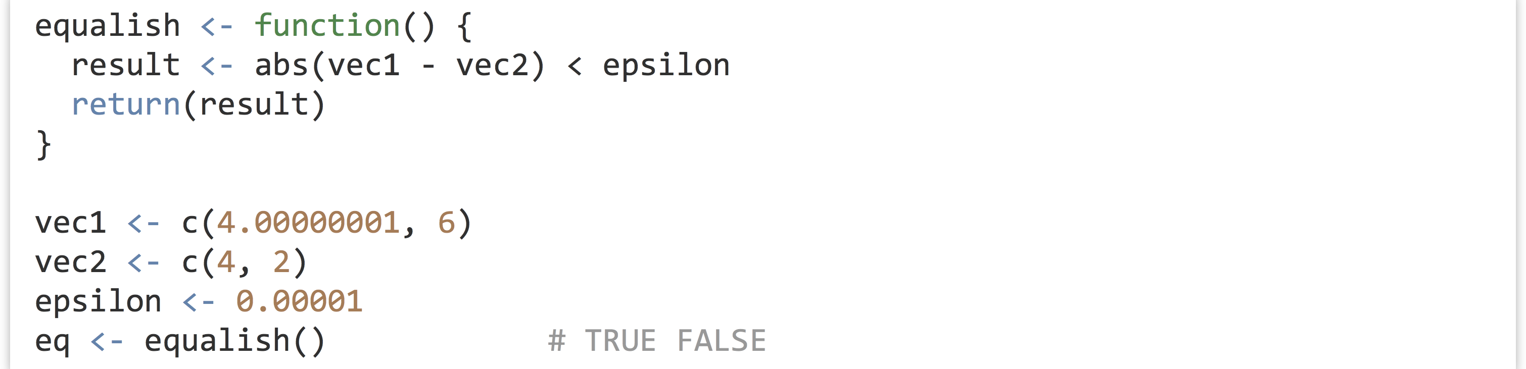
But writing such functions is fairly bad practice. Why? Because although the function still cannot affect the external environment, it is now quite dependent on the state of the external environment in which it is called. The function will only work if external variables called vec1, vec2, and epsilon happen to exist and have the right types of data when the function is called. Consider this: the former version of the function could be copied and pasted into an entirely different program and still be guaranteed to work (because the a and b parameters are required local variables), but that’s not the case here.
The same four “rules” for designing functions in Python apply to R:
- Functions should only access local variables that have been assigned within the function block, or have been passed as parameters (either required or with defaults).
- Document the use of each function with comments. What parameters are taken, and what types should they be? Do the parameters need to conform to any specification, or are there any caveats to using the function? Also, what is returned?
- Functions shouldn’t be “too long.” This is subjective and context dependent, but most programmers are uncomfortable with functions that are more than one page long in their editor window. The idea is that a function encapsulates a single, small, reusable idea. If you do find yourself writing a function that is hard to read and understand, consider breaking it into two functions that need to be called in sequence, or a short function that calls another short function.
- Write lots of functions! Even if a block of code is only going to be called once, it’s ok to make a function out of it (if it encapsulates some idea or well-separable block). After all, you never know if you might need to use it again, and just the act of encapsulating the code helps you ensure its correctness and forget about it when working on the rest of your program.
Argument Passing and Variable Semantics
So far, the differences we’ve seen between Python and R have mostly been in R’s emphasis on vectorized operations. In later chapters, we’ll also see that R emphasizes the creative use of functions more strongly than does Python (which should at the very least be a good reason to study them well).
There is another dramatic difference between these two languages, having to do with variables and their relationship to data. This is probably easiest to see with a couple of similar code examples. First, here’s some Python code that declares a list of numbers nums, creates a new variable based on the original called numsb, modifies the first element of numsb, and then prints both.
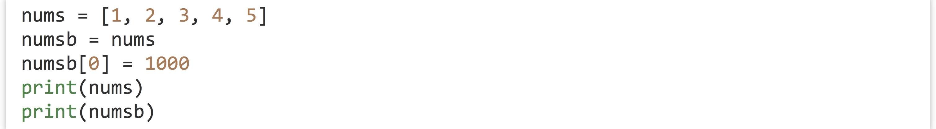
The output indicates that nums and numsb are both variables (or “names,” in Python parlance) for the same underlying data.

Corresponding R code and output reveals that R handles variables very differently:
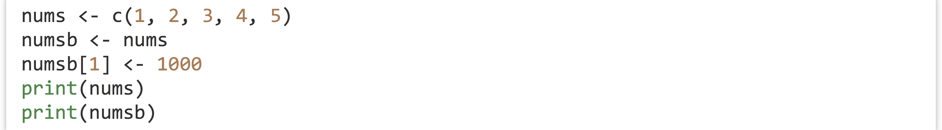

While in Python it’s common for the same underlying data to be referenced by multiple variables, in R, unique variables are almost always associated with unique data. Often these semantics are emphasized in the context of local variables for functions. Here’s the same thing, but the operation is mediated by a function call. First, the Python version and output:
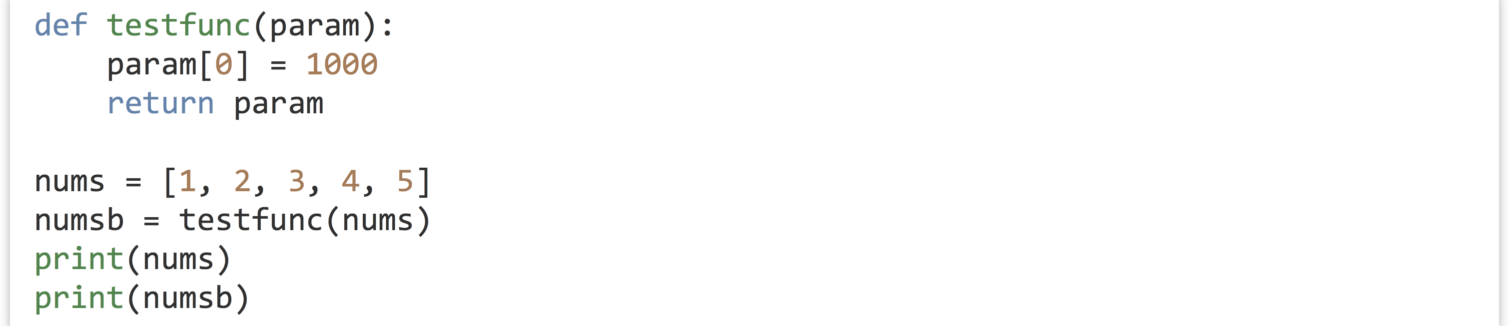

And now the R version and output:
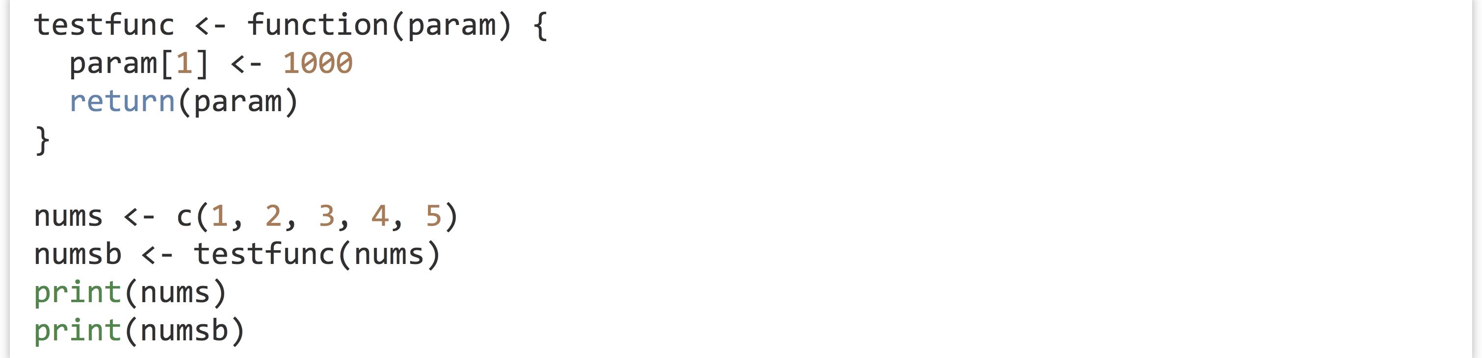

In the Python code, the param local variable is a new variable for the same underlying data, whereas in the R code the local param variable is a new variable for new underlying data. These two paradigms are found in a wide variety of languages; the latter is known as “pass-by-value,” though one could think of it as “pass-by-copy.” This doesn’t mean that R always creates a copy–it uses a “copy-on-write” strategy behind the scenes to avoid excess work. As for the former, the Python documentation refers to it as “pass-by-assignment,” and the effect is similar to “pass-by-reference.” (The term “pass-by-reference” has a very narrow technical definition, but is often used as a catch-all for this type of behavior.)
There are advantages and disadvantages to both strategies. The somewhat more difficult scheme used by Python is both speedier and allows for more easy implementations of some sophisticated algorithms (like the structures covered in chapter 25, “Algorithms and Data Structures”). The pass-by-value scheme, on the other hand, can be easier to code with, because functions that follow rule 1 above can’t surreptitiously modify data: they are “side effect free.”
Getting Help
The R interpreter comes with extensive documentation for all of the functions that are built-in. Now that we know how to write functions, reading this documentation will be easy.
The help page for a particular function can be accessed by running help("function_name") in the interactive console, as in help("t.test") for help with the t.test() function.

Alternatively, if the function name contains no special characters, we can use the shorthand ?function_name, as in ?t.test. The help is provided in an interactive window in which you can use the arrow keys to scroll up and down.
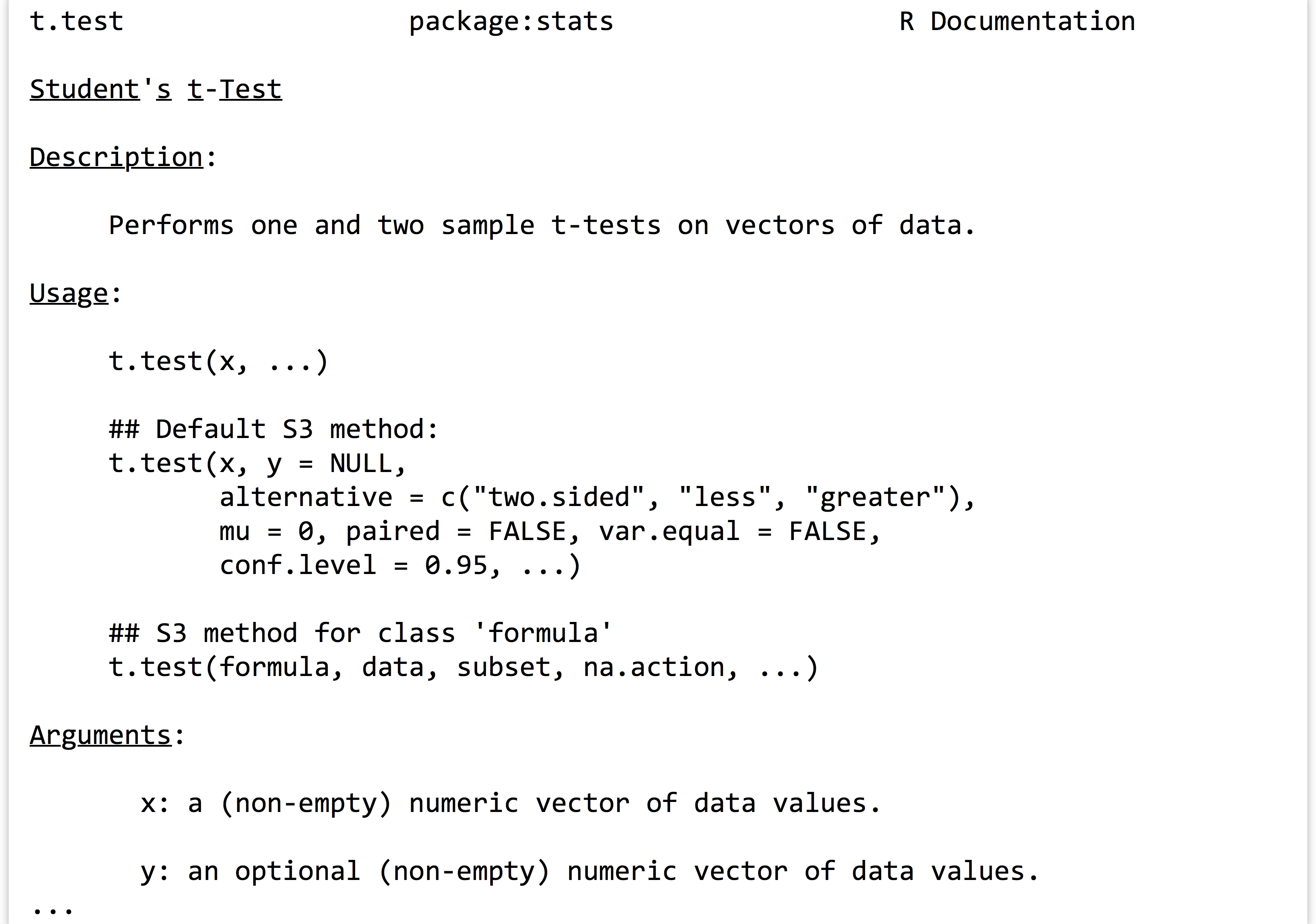
The help pages generally have the following sections, and there may be others:
- Description: Short description of the function.
- Usage: An example of how the function should be called, usually listing the most important parameters; parameters with defaults are shown with an equal sign.
- Arguments: What each parameter accepted by the function does.
- Details: Notes about the function and caveats to be aware of when using the function.
- Value: What is returned by the function.
- References: Any pertinent journal article or book citations. These are particularly useful for complex statistical functions.
- Examples: Example code using the function. Unfortunately, many examples are written for those who are familiar with the basics of the function, and illustrate more complex usage.
- See Also: Other related functions that a user might find interesting.
If a function belongs to a package (such as str_split() in the stringr package), one can either load the package first (with library(stringr)) and access the help for the function as usual (help("str_split")), or specify the package directly, as in help("str_split", package = "stringr"). An overview help page for all functions in the package can be accessed with help(package = "stringr").
Finally, in the interactive window, using help.search("average") will search the documentation for all functions mentioning the term “average”—the shortcut for this is ??average.
Exercises
- We often wish to “normalize” a vector of numbers by first subtracting the mean from each number and then dividing each by the standard deviation of the numbers. Write a function called
normalize_mean_sd()that takes such a vector and returns the normalized version. The function should work even if any values areNA(the normalized version ofNAshould simply beNA). - The
t.test()function tests whether the means of two numeric vectors are unequal. There are multiple versions of t-tests: some assume that the variances of the input vectors are equal, and others do not make this assumption. By default, doest.test()assume equal variances? How can this behavior be changed? - Using the help documentation, generate a vector of 100 samples from a Poisson distribution with the lambda parameter (which controls the shape of the distribution) set to
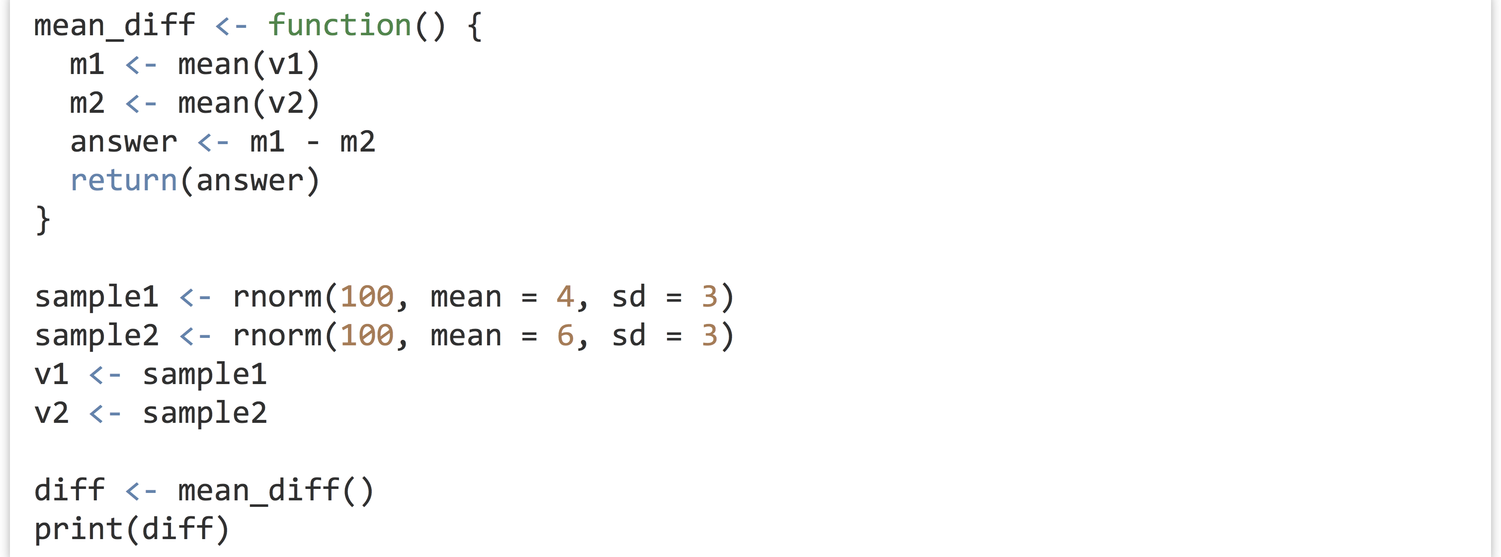
2.0. - The following function computes the difference in mean of two vectors, but breaks at least one of the “rules” for writing functions. Fix it so that it conforms. (Note that it is also lacking proper documentation.)
- The following code generates two random samples, and then computes and prints the difference in coefficient of variation for the samples (defined as the standard deviation divided by the mean). Explain how this code works, step by step, in terms of local variables, parameters, and returned values. What if immediately before
sample1 <- rnorm(100, mean = 4, sd = 2), we hadresult <- "Test message.", and afterprint(answer), we hadprint(result)? What would be printed, and why?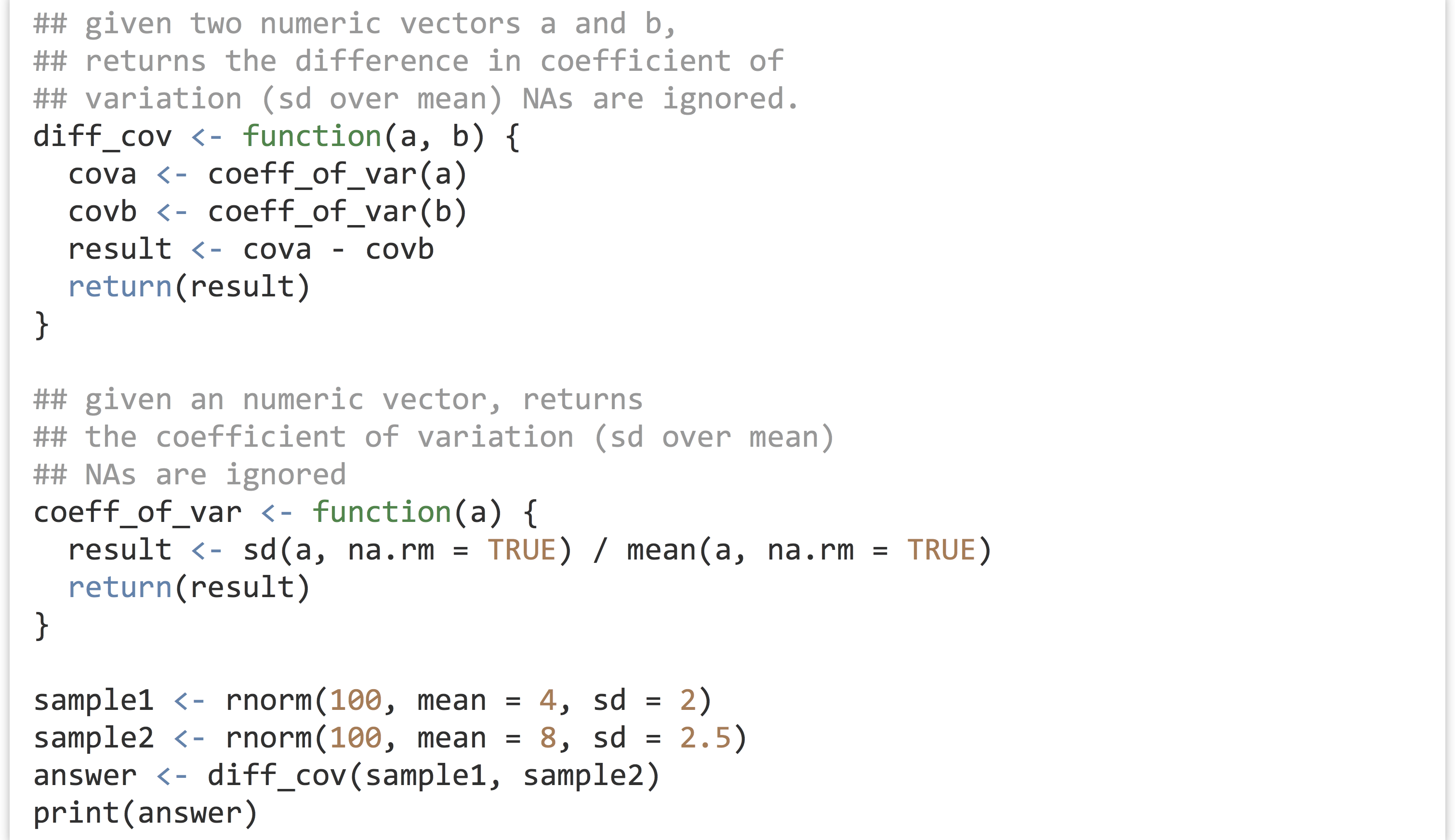
- Any variable that is simply stated (without assignment) in a function will be returned. So, this definition is equivalent:
 Some R programmers prefer this syntax; for this text, however, we’ll stick to using the more explicit
 return(). This also helps differentiate between such “returnless returns” and “printless prints” (see the footnote in Chapter 27, Variables and Data). ↵
