31 Data Frames

In chapter 28, “Vectors,” we briefly introduced data frames as storing tables of data. Now that we have a clear understanding of both vectors and lists, we can easily describe data frames. (If you hastily skipped chapters 28 and 30 to learn about data frames, now’s the time to return to them!) Data frames are essentially named lists, where the elements are vectors representing columns. But data frames provide a few more features than simple lists of vectors. They ensure that the component column vectors are always the same length, and they allow us to work with the data by row as well as by column. Data frames are some of the most useful and ubiquitous data types in R.

While we’ve already covered using the read.table() function to produce a data frame based on the contents of a text file, it’s also possible to create a data frame from a set of vectors.

When printed, the contents of the column vectors are displayed neatly, with the column names along the top and row names along the left-hand side.

As with read.table(), the data.frame() function takes an optional stringsAsFactors argument, which specifies whether character vectors (like ids) should be converted to factor types (we’ll cover these in detail later). For now, we’ll disable this conversion.

Running str(gene_info) reveals the data frame’s list-like nature:

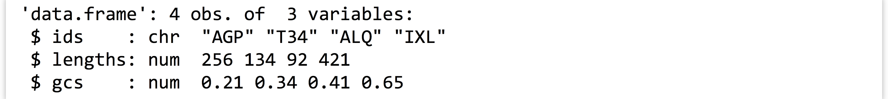
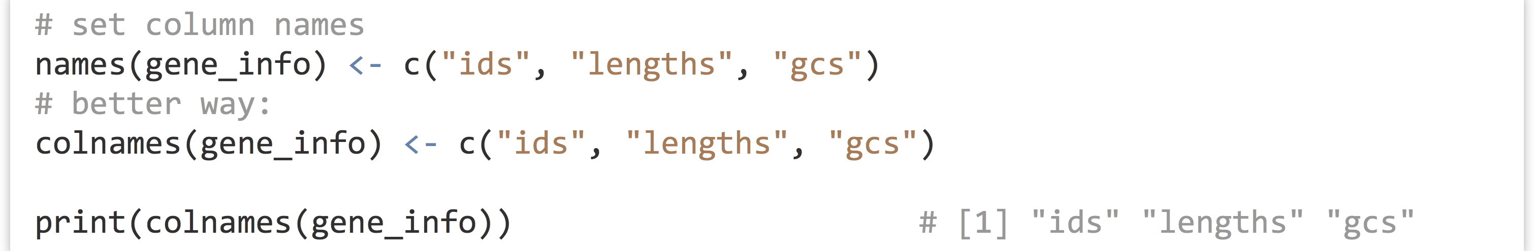
Like elements of lists, the columns of data frames don’t have to have names, but not having them is uncommon. Most data frames get column names when they are created (either by read.table() or data.frame()), and if unset, they usually default to V1, V2, and so on. The column names can be accessed and set with the names() function, or with the more appropriate colnames() function.

To highlight the list-like nature of data frames, we can work with data frames by column much like lists by element. The three lines in the following example all result in sub_info being a two-column data frame.

An expression like gene_info[2] thus would not return a numeric vector of lengths, but rather a single-column data frame containing the numeric vector. We can use [[]] syntax and $ syntax to refer to the vectors contained within data frames as well (the latter is much more common).

We can even delete columns of a data frame by setting the element to NULL, as in gene_info$lengths <- NULL.

The real charm of data frames is that we can extract and otherwise work with them by row. Just as data frames have column names, they also have row names: a character vector of the same length as each column. Unfortunately, by default, the row names are "1", "2", "3", and so on, but when the data frame is printed, the quotation marks are left off (see the result of print(gene_info) above). The row names are accessible through the rownames() function.

Data frames are indexable using an extended [] syntax: [<row_selector>, <column_selector>], where <row_selector> and <column_selector> are vectors. Just as with vectors and lists, these indexing/selection vectors may be integers (to select by index), characters (to select by name), or logicals (to select logically). Also as with vectors, when indexing by index position or name, the requested order is respected.

Here’s the resulting output, illustrating that "3" and "1" were the row names, which now occur at the first and second row, respectively. ^[1]

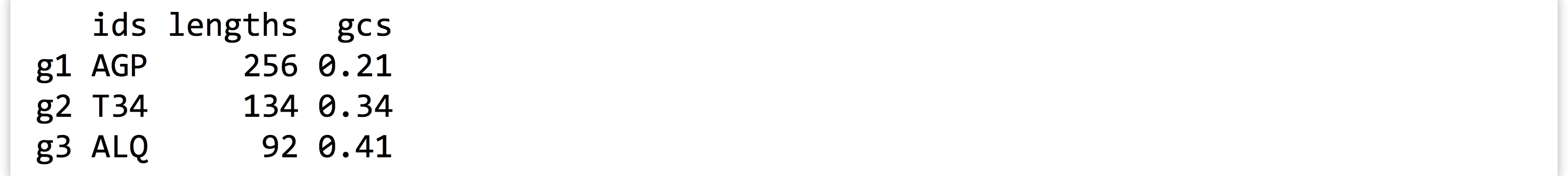
If you find this confusing, consider what would happen if we first assigned the row names of the original data frame to something more reasonable, before the extraction.

Now, when printed, the character nature of the row names is revealed.

Finally, if one of <row_selector> or <column_selector> are not specified, then all rows or columns are included. As an example, gene_info[c(3,1), ] returns a data frame with the third and first rows and all three columns, while gene_info[, c("lengths", "ids")] returns one with only the "lengths" and "ids" columns, but all rows.

Data Frame Operations

Because data frames have much in common with lists and rows—and columns can be indexed by index number, name, or logical vector—there are many powerful ways we can manipulate them. Suppose we wanted to extract only those rows where the lengths column is less than 200, or the gcs column is less than 0.3.

This syntax is concise but sophisticated. While gene_info$lengths refers to the numeric vector named "lengths" in the data frame, the < logical operator is vectorized, with the single element 200 being recycled as needed. The same process happens for gene_info$gcs < 0.3, and the logical-or operator | is vectorized, producing a logical vector later used for selecting the rows of interest. An even shorter version of these two lines would be selected <- gene_info[gene_info$lengths < 200 | gene_info$gcs < 0.3, ]. The printed output:

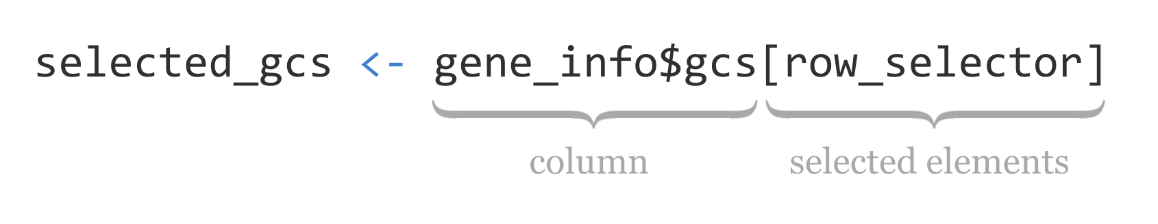
If we wished to extract the gcs vector from this result, we could use something like selected_gcs <- selected$gcs. Sometimes more compact syntax is used, where the $ and column name are appended directly to the [] syntax.

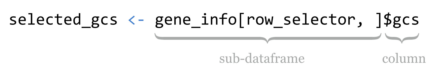
Alternatively, and perhaps more clearly, we can first use $ notation to extract the column of interest, and then use [] logical indexing on the resulting vector.

Because subsetting data frame rows by logical condition is so common, there is a specialized function for this task: subset(). The first parameter is the data frame from which to select, and later parameters are logical expressions based on column names within that data frame (quotation marks are left off). For example, selected <- subset(gene_info, lengths < 200 | gcs < 0.3). If more than one logical expression is given, they are combined with & (and). Thus subset(gene_info, lengths < 200, gcs < 0.3) is equivalent to gene_info[gene_info$lengths < 200 & gene_info$gcs < 0.3 ,].

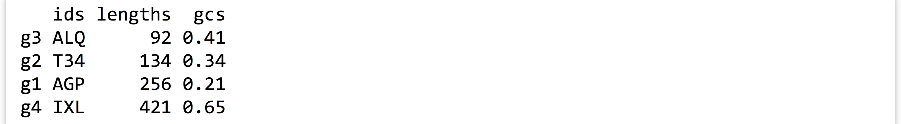
While the subset() function is convenient for simple extractions, knowing the ins and outs of [] selection for data frames as it relates to lists and vectors is a powerful tool. Consider the order() function, which, given a vector, returns an index vector that can be used for sorting. Just as with using order() to sort a vector, we can use order() to sort a data frame based on a particular column.

The result is a data frame ordered by the lengths column:

Because data frames force all column vectors to be the same length, we can create new columns by assigning to them by name, and relying on vector recycling to fill out the column as necessary. Let’s create a new column called gc_categories, which is initially filled with NA values, and then use selective replacement to assign values "low" or "high" depending on the contents of the gcs column.

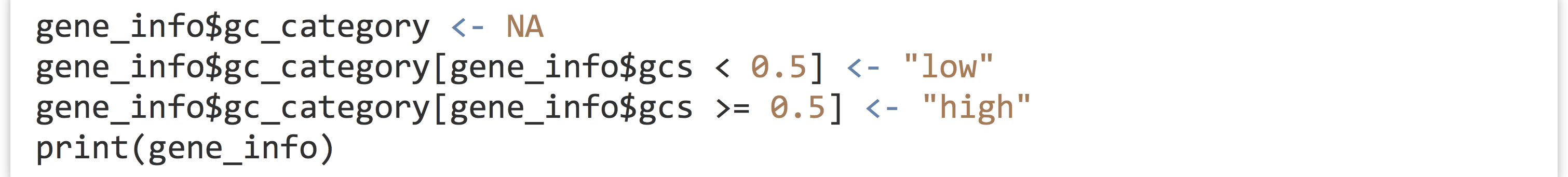
While there are more automated approaches for categorizing numerical data, the above example illustrates the flexibility and power of the data frame and vector syntax covered so far.

One final note: while the head() function returns the first few elements of a vector or list, when applied to a data frame, it returns a similar data frame with only the first few rows.