Population ecology provides scientists and managers with information on populations of species that can indicate that population’s sustainability over time and the degree to which the species utilizes the available habitat.

Section 1: Demography

A population is the total of the individuals of a given species living in a given area. Examples are the population of sage grouse in one hundred acres of sagebrush steppe or all the individuals of the Gunnison sage grouse throughout the western United States. The study of how a population of a given species changes over time is referred to as demography. Changes studied can include population size, population density, species distribution, sex ratios, births, deaths, or any characteristic that describes the entire population under study or management.

Population Size and Density

Population size is the number of individuals of a species in a given area. Population density is the number of individuals per unit area. For plant species and many animal species, these numbers are estimates obtained using sampling methods. For example, if we want to know the population density of big basin sagebrush (Artemisia tridentata) we might lay out a quadrat (an area of a given size, such as a meter or an acre) and count all the individuals of the species within that quadrat. This sampling method is conducted randomly throughout the study area, then statistics are used to estimate the population. If we want to know the population size of pronghorn, we might use visual observation counts from random sites or from the same site over a period of time (days to weeks) and then use statistical analysis to estimate the population size. Another common method in wildlife population counts is mark and recapture.

Population and density size tell us several things about the species and the ecosystem such as the following:

1. The population’s degree of stability. Larger populations tend to be more stable as they can absorb a certain threshold of increase or decrease in population size. Larger populations also have a greater degree of phenotypic plasticity and a greater ability to adapt to environmental shifts.
2. Habitat availability in some instances can be one indicator of the ecosystem function and structure in a given area.
3. Population size is directly dependent on the carrying capacity of a given area.
4. Among wildlife and with livestock, population size informs dietary overlap.
5. In general, humans are most interested in species’ population size in relation to humans or human activity, such as conservation efforts, hunting, endangered species survival, and so on.

Species Distribution

Species distribution is how individuals of a population are distributed across a given area and reflects species dispersal methods and population interactions. There are three general distribution types:

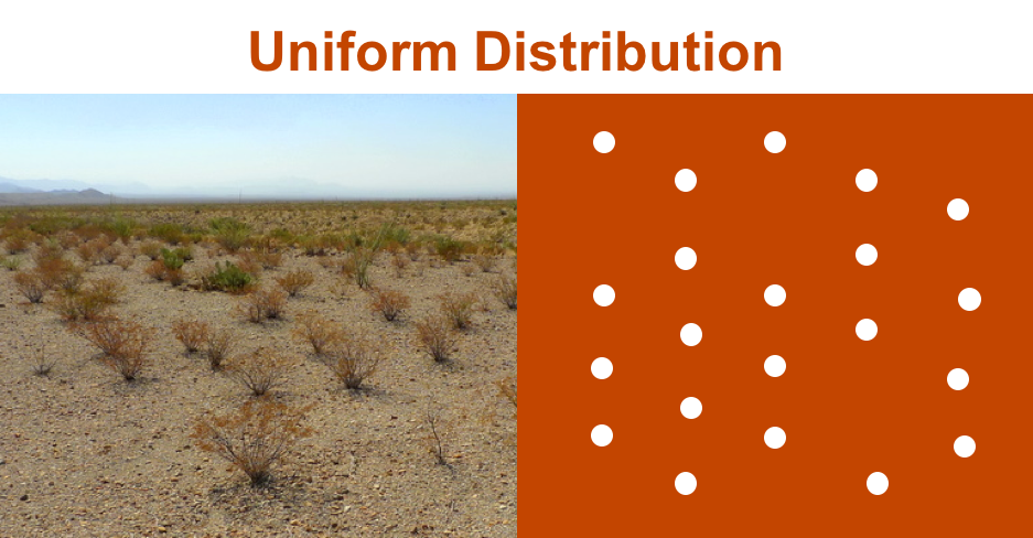
In uniform distribution, individuals are spaced uniformly across a given area. It is fairly easy to recognize a population of creosote bushes (Larrea tridentata) from a distance, as shown in figure 3.1, for example, because of their allelopathic effect (fibrous roots just below the soil surface spread out and release a toxin that inhibits the growth of other plants).

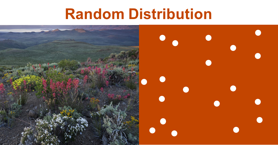
Individuals in random distribution are spaced across a given area without any predictable pattern, as shown in figure 3.2. The least frequently seen type of distribution, random distribution is not much influenced by ecosystem dynamics. Typical species with this type of distribution are plant species with wind-driven seed dispersal, such as a dandelion.

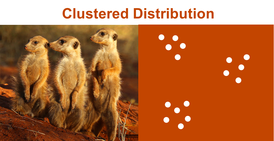
In clustered distribution, the most common distribution type, individuals clump in groups across a given area, as shown in figure 3.3. Clustered distribution is driven by species biology and ecosystem dynamics. Plants, such as aspen trees, that reproduce vegetatively expand outward from the cluster. Herd animals, such as pronghorn, are distributed in clusters in the proximity of available habitat. Pack animals, such as wolves, distribute in clusters in defined territories with the carrying capacity to support their density.

Species Birth and Death Rates, Age-Sex Structure, and Survivorship Curves

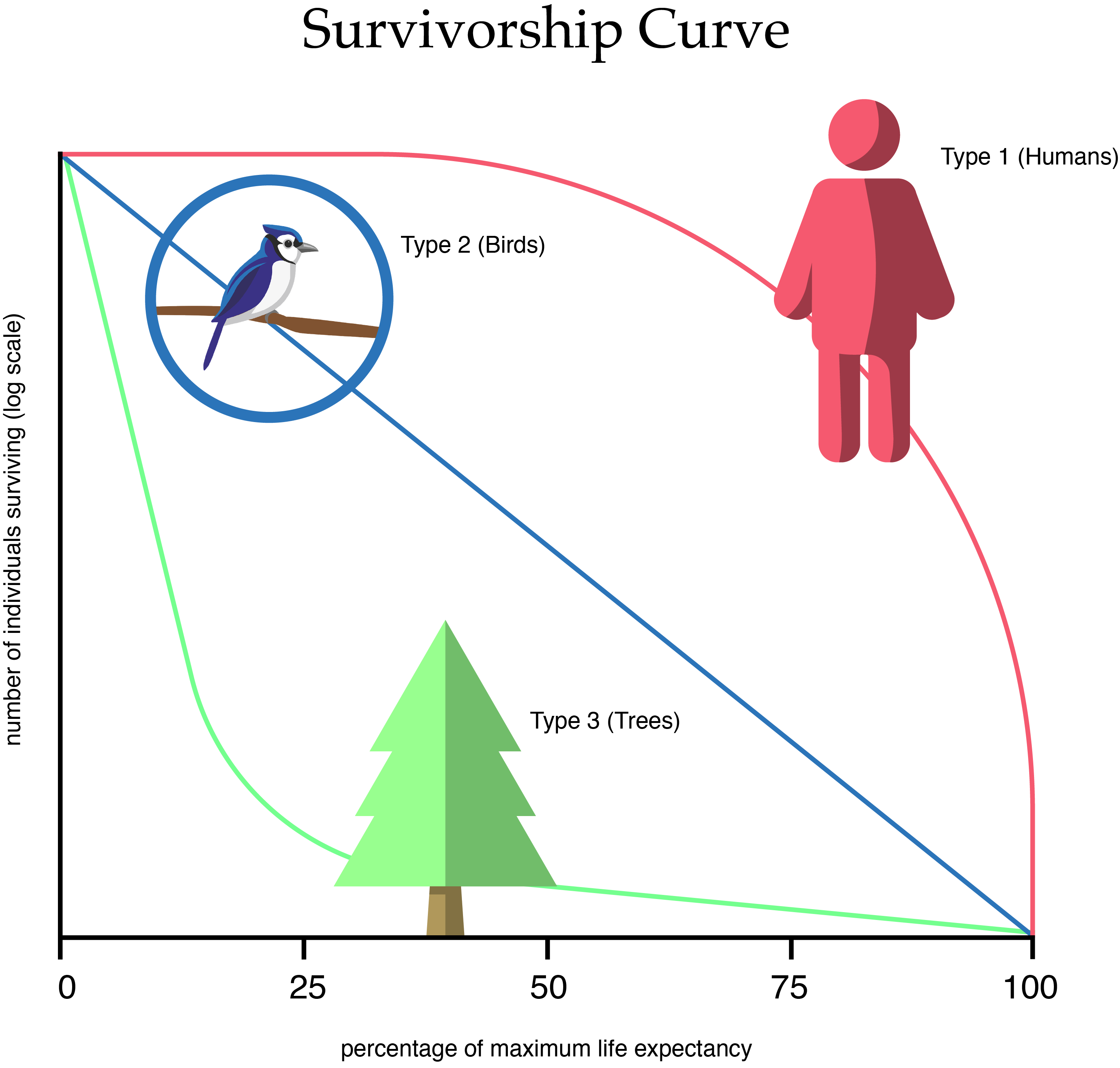
Life tables, age-sex structures, and survivorship curves can indicate the likelihood of whether a population will grow or contract in the near future.

Life tables are comprised of birth and death data. These tables convey reproduction rates and death rates, as well as age of death, thus indicating the age at which individuals of a species are at highest risk of death. This information can guide conservation planning and underlies survivorship curves.

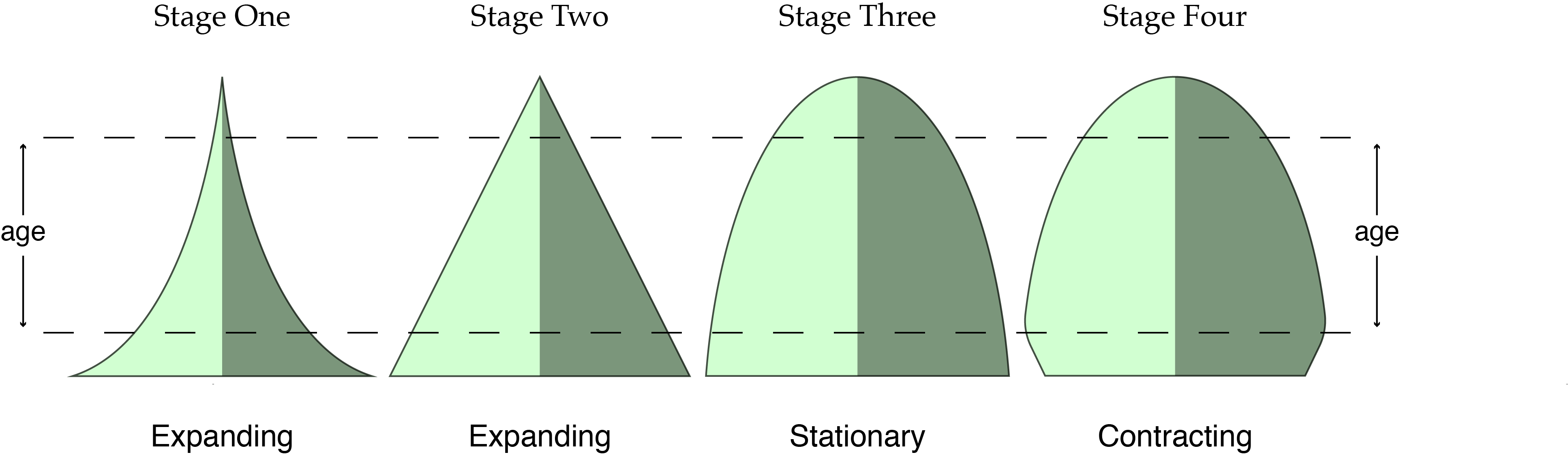
Survivorship curves, tied to life tables, use three types of curves to represent a population’s general duration of life and age of mortality. Knowing the survivorship curve of a species can contribute to predicting its population growth.

Age-sex structure graphs, as shown in figure 3.5, represent age and sex distribution across a population, which indicates a population’s potential to grow or shrink. Age-sex structure combined with life tables can predict the rate at which a population may grow or contract in the future.

Section 2: Population Growth and Control

In the previous section, we noted that populations grow and contract and that monitoring growth and contractions can guide management efforts. Managing populations, however, requires understanding the multitude of factors underlying population growth and contraction. The many factors that can influence fluctuations in population size and density are generally divided into two categories: density dependent and density independent.

Density Dependence

If resources are unlimited, populations will grow at an unlimited geometric rate (if reproduction is periodic, with the population going through the reproduction cycle annually; deer are an example) or at an unlimited exponential rate (if reproduction is continuous, with individuals in a population reproducing at any time; rabbits, for example). In reality, resources are not unlimited, and at some point carrying capacity (the maximum number of individuals a system’s resources can support) is reached, and population growth slows or declines. When carrying capacity is reached, sustained birth and death rates must be balanced to limit population growth unless more resources become available either through migration of individuals out of the population or through expansion of the population habitat. Thus density dependence indicates regulation of population size based on population size related to carrying capacity.

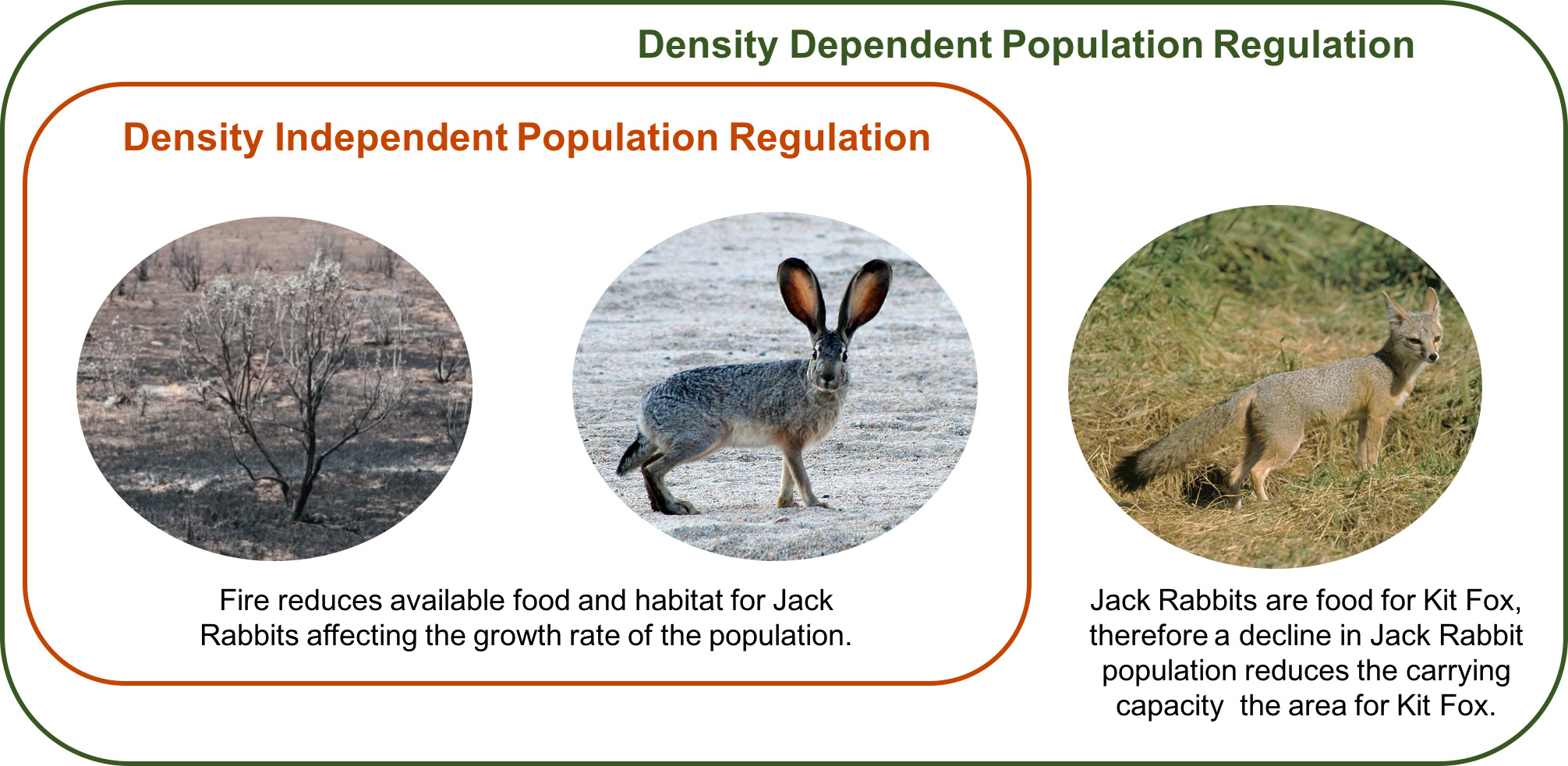
Density Independence

Density-independent population regulation may be driven by environmental factors, such as drought or wildfire, or by community dynamics, such as predation or allelopathy.

Factors favoring density dependence and density independence can interplay, resulting in fluctuations in population growth and contraction.

Section 3: Influences on Population Dynamics and Distribution

A multitude of abiotic, biotic, and disturbance factors can influence population dynamics, and this section examines a few of the dominant and most concerning ones.

Abiotic Factors

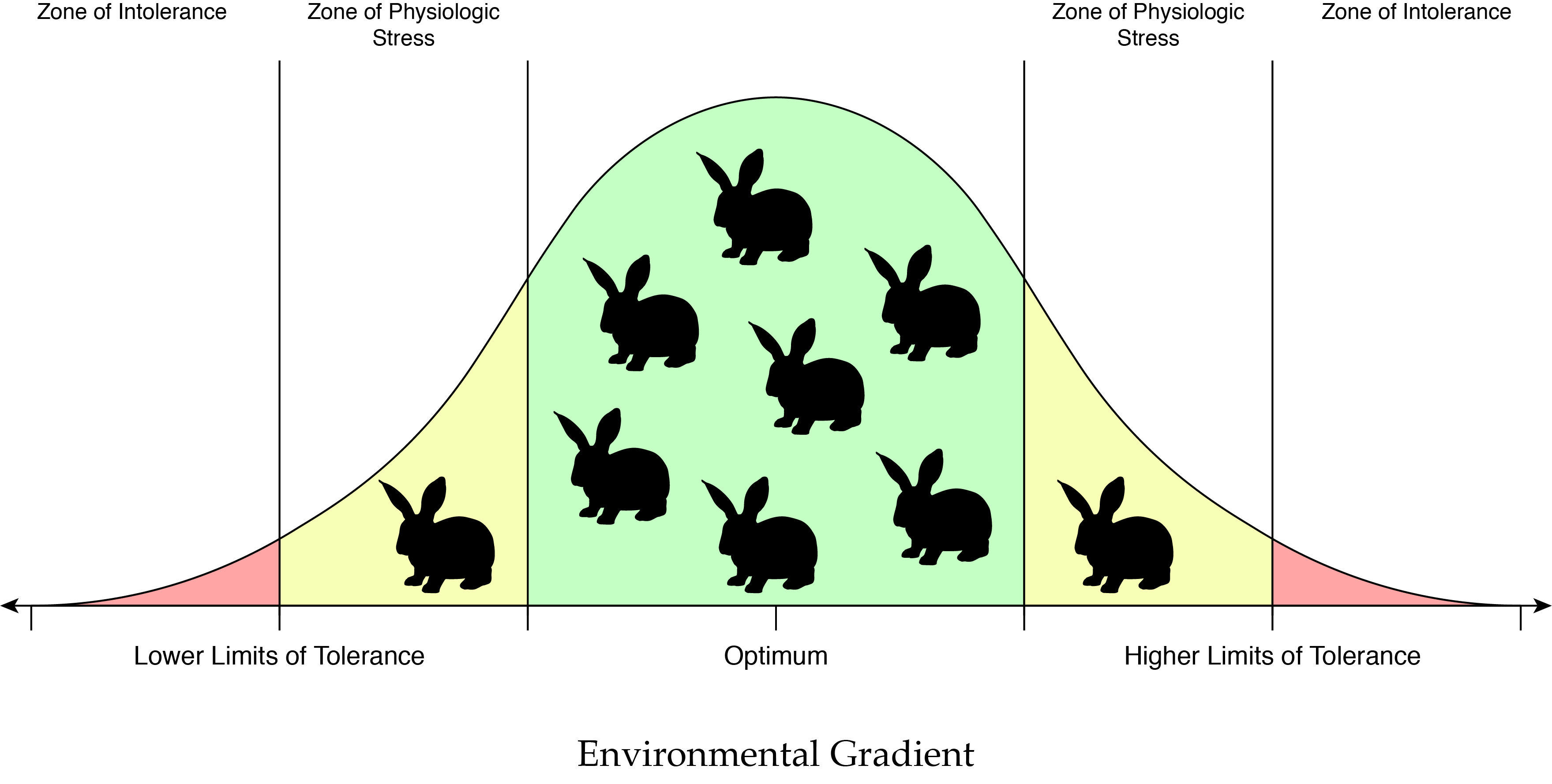
Two primary abiotic factors influence population dynamics and distribution: physical geography and climate. A third factor, specific to plants, is soil. Physical geography includes physical barriers, such as mountain ranges and bodies of water, that influence establishment, dispersal, and distribution. If a species cannot physically move over or around a mountain, wide-open space, or body of water, its range is bounded. Species may also be temporarily constrained by disturbances, such as a fire or flood. Fire, for example, may temporarily remove vegetative cover needed as shelter or protection or alter soil chemistry and water infiltration, diminishing a food source or soil accessibility for burrowing animals.

Physical barriers also create climatic conditions and environmental gradients. Environmental gradients of temperature, precipitation, soil texture, water, or chemistry can all create physical barriers that confine a population. As discussed in chapter 2, species have a niche that includes the range of environmental conditions they can tolerate. Species generally inhabit a range of optimal conditions and exist at decreasing population levels under the stresses toward the edges of that range.

Disturbance often constrains a species’ range by shifting the temperature, precipitation, soil texture, and nutrient cycling gradients.

Biotic Factors: Species Interactions

Species distribution can also or additionally be constrained by species interaction factors, such as allelopathy, predation, competition, and mutualism. These will be briefly covered here and in more depth in chapter 4: Ecological Systems Thinking.

Allelopathy

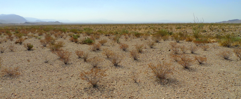
Plants using allelopathy excrete a chemical substance that inhibits the growth of other plants. Driving through the Mojave and Chihuahuan Deserts the distribution pattern of a certain shrub, the creosote bush (Larrea tridentata), seen in figure 3.8, becomes noticeable. The creosote bush diminishes competition through allelopathy.

Predation

The abundance of predators may encourage prey to constrain their movements, while a low population of prey may encourage a predator to expand its niche within its range. For example, in eastern Oregon use of radio collars has documented that if wolves (Canis lupus) are present, black-tail deer (Odocoileus hemionus) as well as cattle restrict their movement across a landscape (Clark et al. 2017a).

Competition

Competition occurs among many species, both plants and animals. A frequently noted competition is the dietary overlap between cattle and other grazing ungulates. It has been documented that black-tail deer (Odocoileus hemionus) and elk (Cervus canadensis) will not graze or browse in an area occupied by cattle.

Invasive species compete for resources with native plants, and as an invasive species becomes dominant it constrains the local range of native species. Cheatgrass (Bromus tectorum) has restricted the distribution of native bunchgrasses, such as Idaho fescue (Festuca idahoensis) and bluebunch wheatgrass (Pseudoroegneria spicata), throughout the Columbia Basin.

Competition is not always based solely on dietary overlap; it may also involve food for one species and habitat for another. For example, the threatened sage grouse (Centrocercus urophasianus) does not directly compete with cattle for food; rather, it competes for the vegetation structure it requires for mating and nesting.

Mutualism

The phrase “pollinators in peril” reflects the mutualistic relationship between plants and pollinators and the increasing concern that species reproduction and dispersal are being diminished by a reduction in pollinator populations. Reduced reproduction and dispersal capacity can constrain a species within its range.

Disturbance: Invasive Plants

Disturbances, particularly invasive plant proliferation, have greatly influenced native plant and animal populations throughout the western United States. On landscapes disturbed by land uses such as grazing, urbanization, conversion to agriculture, and recreation, and environmental events such as drought and fire, invasive plants are able to establish themselves in resource-limited niches and then outcompete native species, proliferating to the point of dominating a system and thus degrading its biotic integrity; in many cases, soil stability and hydrologic function are degraded as well. Degradation creates ripple effects not only in vegetation composition but also in microbial, insect, and wildlife habitat, with concomitant population decline.

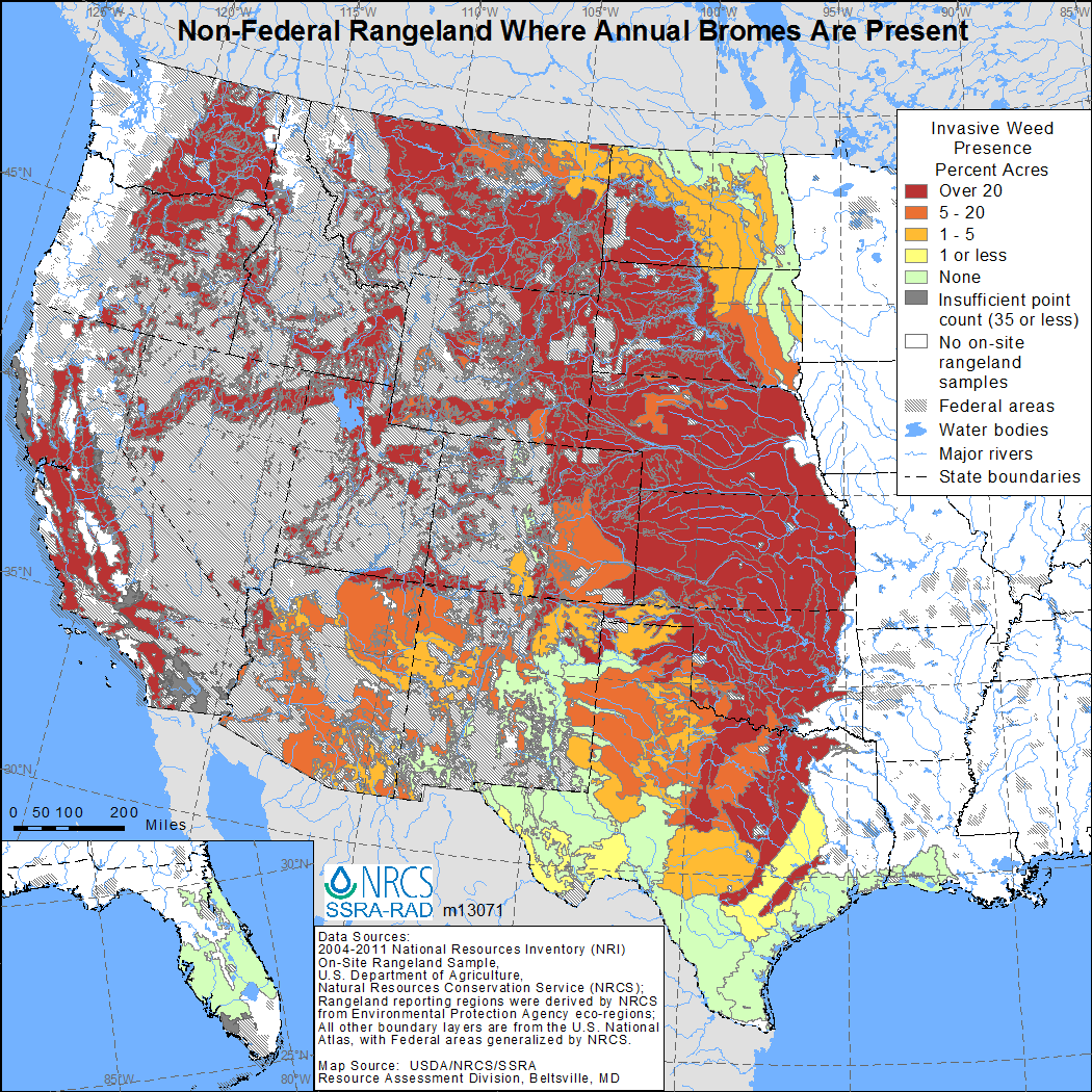
One of the most widespread and impactful groups of invasive species is annual bromes. Figure 3.9 maps the intensity of annual brome distribution on nonfederal land throughout the West. The dominant red shading indicates that for each acre, over 20 percent of the vegetation population is annual brome species. A map of federal lands would reflect a similar extent and intensity of annual brome populations. The dominance of annual bromes throughout the West contributes to reduced populations of wildlife species (e.g., sage grouse); increased fire risk; reduced hydrologic function; reduced grazing capacity; and reduced capacity of many other ecosystem goods and services. Other invasive species, such as thistles, knapweeds, and spurges, have similar impacts on vegetation and wildlife communities. Chapters 6 and 8 of this text will discuss ecological, economic, and social impacts of invasive species in more detail.

Influence of Climate Change

Climate change is the shifting in variation, intensity, and global distribution of climatic factors such as precipitation, temperature, wind, pressure fronts that create storm systems, and others. For example, an area that in recent history experienced summer maximum temperatures in the 80°F range may currently be experiencing summer maximum temperatures in the 90°F range (IPCC 2007). Areas that received on average two feet of snowfall from December through March now receive less than a foot of snowfall, while areas that generally do not receive snowfall are recording multiple winter storm events averaging four to six inches of snowfall (IPCC 2007). These are pronounced events and shifts. In addition, subtle shifts occur at different geographic scales from a few square miles to large geographic regions (IPCC 2007).

These types of shifts can greatly influence the distribution and density of plants and animals. Since biogeography is based on climate and geology, shifts in climate will result in biogeographic shifts for some species over time. One of the most evident shifts in the rangeland systems that are the focus of this text is occurring in C3 and C4 species. Recall that C3 species are cool-season species (growth cycle starts in fall and ends in summer), and C4 species are warm-season species (growth cycle starts in spring and ends in fall). The strategic difference between C3 and C4 species is based in photosynthesis and optimal growth conditions. C3 plants begin growing when soil temperature is 40–45°F, and their optimum temperature range for growth is 65–75°F, after which plant production becomes less efficient and diminishes (IPCC 2007). The soil temperature range for growth initiation of C4 plants is twenty degrees higher (60–65°F), and the optimum temperature for growth is twenty to thirty degrees higher (90–95°F). Additionally, C4 plants also require less water for plant physiological processes. Therefore, the range for C4 plants is expanding as atmospheric carbon and temperatures increase.

Chapter 4 will explore the complex interrelationships among biotic and abiotic system components in the context of the influences of climate change on populations. We will examine how a shift in C3 and C4 species influences shifts in populations of other species and community interaction dynamics.

Conclusion

In chapter 2 we focused on specific adaptations of plants and animals for survival under the environmental stress of heat and aridity. In this chapter, we focused on factors that influence species survival, growth, and distribution. The concepts we learned in these two chapters will underlie our understanding of community ecology—how populations of species interact and influence one another—which is the focus of chapter 4.