Introduction

Before we can even begin to discuss cells, it’s important to understand that cells are very tiny! Most cells are too small to see with the naked eye. Thus, the beginning of our book must start with a conversation about microscopes and how they work. An understanding of the tools we use to study cells, both their abilities and their limitations, is essential to making sense of the material you’re going to be exploring throughout this book. These days, thanks to some pretty impressive advances in computing in the last 50 years or so, there are a great many different types of microscopes that exist. We can’t possibly cover all of the different kinds with the time that we have to cover this topic. However, the essence of all of the varied types of microscopes that are used to explore cell biology fit into four major groupings:

1. Brightfield light microscopy
2. Fluorescene light microscopy
3. Transmission electron microscopy (TEM)
4. Scanning electron microscopy (SEM)

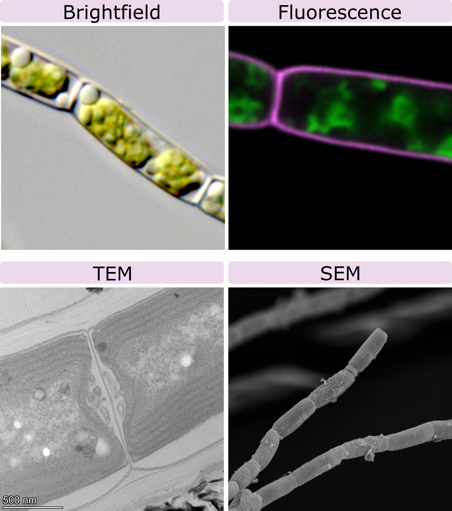
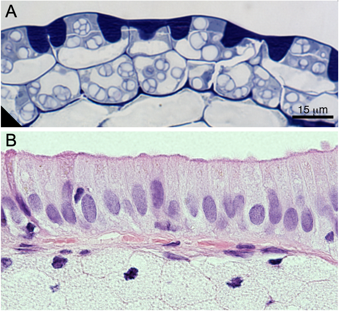
The capacity to visualize samples in any kind of microscope depends on the particle that is used by that microscope. The first and oldest microscopes were developed about 400 years ago and used visible light from the sun, with glass lenses to magnify the sample. About 80–100 years ago, we discovered that using electrons to image samples greatly increased both the magnification and resolution of the microscope. These days, both light and electron microscopy are still in use. We will look at each type of microscopy in turn and explore their strengths and limitations. An example of each is included in Figure 01-01 for direct comparison in the same organism. We will also show more examples throughout the chapter. Consider how we might identify each type of microscopy and distinguish when we could use one type over the other. However, before we do any of that, we must first discuss the concepts of magnification and resolution, since all microscopes use both to help us see very small objects, like cells.

Topic 1.1: Magnification and Resolution

Before we take a deeper dive into the topic of microscopy, it may be useful to revisit the physics behind how microscopes work. It’s important to understand the basic principles of the wave/particle properties of visible light, which is one small section of the electromagnetic spectrum. Electrons also have both wave and particle-like properties, so many of the principles that underlie electron microscopy are similar to those that underlie light microscopy. Fluorescence microscopy and scanning electron microscopy (SEM) are derivatives of the other two, in which the source of the particle and/or the way the particle is detected is changed so that a different image is created.

All microscopes have limitations on the size and detail with which they can be used to visualize objects. These limitations are a product of the specific characteristics of the particle being used to create the image (i.e., photons or electrons). The wavelength at which these particles travel has a direct impact on how much detail can be seen in the image generated. When discussing the limitations of microscopes, we generally discuss them in terms of magnification and resolution.

The Merriam-Webster Dictionary defines magnification as “the apparent enlargement of an object by an optical instrument.” In other words, a microscope allows us to make very tiny things look bigger than they are. The objectives on a standard classroom microscope often tell you their magnifying power so that you have some context for the actual size of the things that you can see using the lens.

On the other hand, resolution is defined as the closest spacing of two lines that can be distinguished as separate entities. The resolution of any microscope is limited by the wavelength of the particle being used to illuminate it. In the case of the light microscope, the resolution (d) is

[latex]\text{d} = 0.61 * \text{wavelength}/\text{numerical aperture of the objective.}[/latex]

If we consider that the shortest wavelength of light that we can see (violet) is about 400 nm, then our calculation for the resolution of a standard light microscope is as follows:

A standard 63× magnification oil-immersion lens (often the highest magnification available in those classroom microscopes) has a numerical aperture of 1.4. So based on this, the resolution of a standard classroom light microscope with that objective would be 0.61*400 nm/1.4, which equals about 175 nm, or roughly 0.2 µm.

This is pretty small. At that range, we can probably see bacteria and maybe even some large viruses (but not all and definitely not well). We also can see some of the larger subcellular organelles in a cell (like the nucleus and mitochondria), but not much of the smaller organelles. Also, any structure that we can see that’s close to the limit of resolution of the light microscope won’t have much detail visible. Much like if you see someone who is very far away, you may only be able to tell that they are a human, but not if it’s someone that you know.

Electrons, on the other hand, have a much shorter wavelength than photons of the visible light spectrum…roughly 200,000 times smaller! Because of that, the resolution limit of an electron microscope is much smaller…there are some kinds of electron microscopes that can view individual atoms! More commonly, in the more widely used electron microscopes, the resolution limit is roughly 0.1 nm. A single double helix of DNA is 2 nm in diameter, and the thickness of the average lipid bilayer is between 4 and 10 nm. We can see both of these in an electron microscope. As such, we can see that this resolution limit is small enough that a lot of the finer structural details inside the cell become visible.

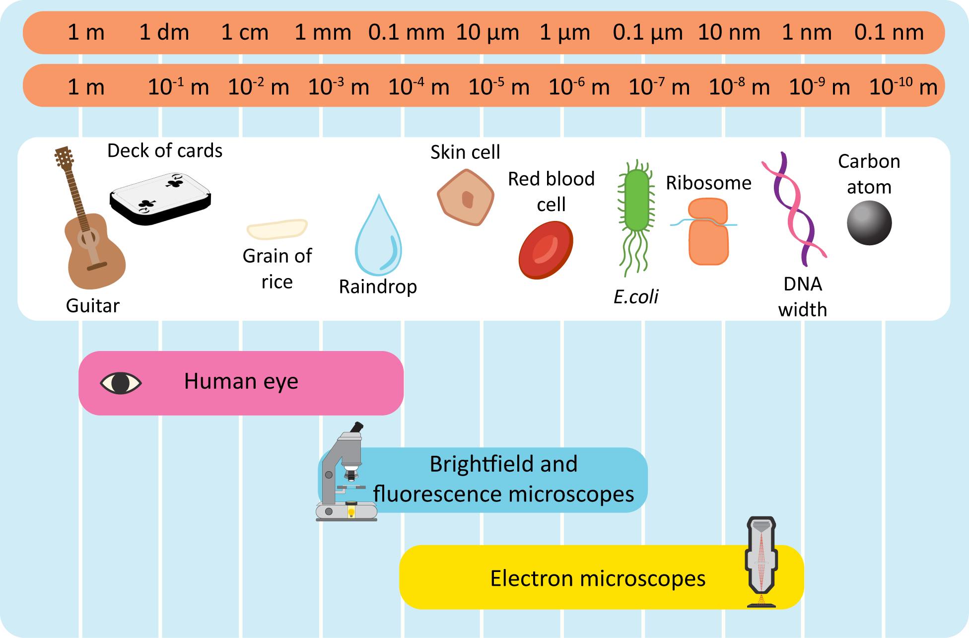
Figure 01-02 gives a rough estimate of what we can see using light or electron microscopy. The website Size of the Universe is also worth exploring. It shows examples that range from the largest thing known (the entire observed universe, or ~10²⁷m) down to the smallest theoretical measurable length in the universe (Planck’s length, or 10^-35m).

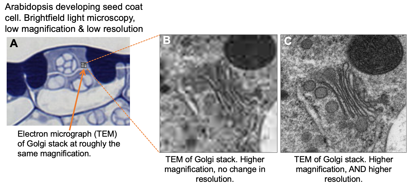
It’s important to remember that resolution is a quality that is separate from magnification. The magnification of an image is simply how much we have enlarged the object in order to observe it. For example, if you wanted to blow up a photo to hang on your wall, you would have to increase the magnification in order to do so. If there aren’t enough pixels in your image to support the amount that you’re magnifying it, then at some point the quality of the image will decrease as you increase the magnification. You can’t actually see more detail; you just see the pixels more obviously. The number of pixels the image contains will determine how much detail you can see. Thus, the number of pixels dictates the resolution of the image that you can create, especially as you blow the image up larger and larger. Applying this to microscopy, in order to see small structures, you not only have to have a higher magnification in order to zoom in, but you also need higher resolution in order to see the details of the smaller structures. Figure 01-03 shows a comparison of microscopy at the same magnification with different resolution to highlight why increased resolution is required with an increase in magnification.

With microscopes, as with the photos that you take with your phone, it is important that the resolution increases along with the magnification in order to see the details desired in the image. The kinds of microscopy that we will explore have different resolution limits. Thus, the resolution that is required in order to observe the structure that you’re interested in will be a major factor when considering the type of microscopy to use in any given situation.

We will leave the final word on this to the following video, created specifically to help you think about the differences between magnification and resolution and also consider how to interpret images when the microscope requires us to cut the sample into thin sections.

Topic 1.2: Light Microscopy

The very first microscope was made in the mid-1600s by a British man named Robert Hooke. That microscope had a mirror to direct sunlight into the glass lenses of the microscope so that the sample could be viewed. Microscopes stayed more or less the same for the next 300 years, until the Industrial Revolution of the early 1900s. It is at this point that the advances in technology allowed us to greatly improve how microscopes work. Now there are light microscopes that use various combinations of lasers, lenses, spinning discs, and computer algorithms to push beyond what should be possible given the physical limitations of visible light. We’ve also made significant advances in sample preparation, which have made additional contributions to what we can visualize. Even though we have incredibly advanced microscopy techniques with which to view cells, their essence remains the same. We will explore the two largest categories of light microscopes: those that collect transmitted light, originating from some kind of light source, to view the sample and those that collect light that is emitted by the sample itself.

Pros to Light Microscopy

Live cells can be viewed and recorded in real time. Specific structures can be labeled for viewing, thus reducing the “noise” in the sample and showing finer details that may otherwise be masked by other components of the sample.

Cons to Light Microscopy

The limit of conventional (brightfield and confocal microscopy) resolution is about 0.2 µm, which restricts the amount of detail we can see of internal cellular structures using light microscopy.

• There is a newer technique, known as superresolution microscopy, which is technically able to break this barrier. We will discuss this in more detail later.

Transmitted versus Emitted Light

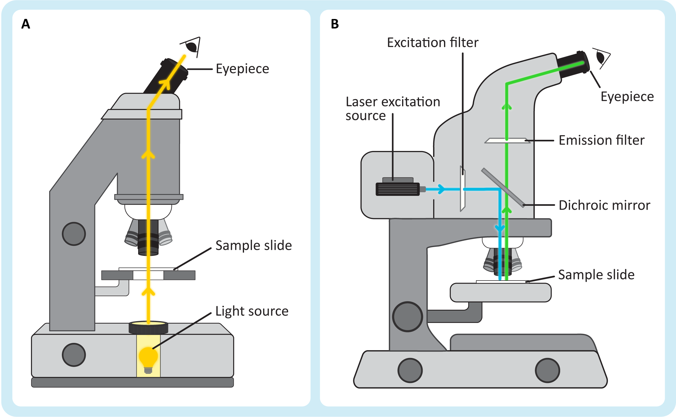
Light microscopy can be further divided into several subtypes of light microscopy. The most notable of these subdivisions takes into account the types of light that you are viewing when you look at an image (Figure 01-04).

• Transmitted light microscopy (Figure 01-04A) is the traditional light microscopy that you most likely tried in high school biology classes. In this type of microscopy, the sample sits between the light source and the eyepiece, and the light you see is the light that was able to pass through the sample. The simplest version, which is the one we will discuss, is called brightfield light microscopy.
• In emitted light microscopy (Figure 01-04B), the sample is illuminated by a light source that is off to the side, and then the molecules in the sample get excited by this light and release their own photons. Thus, the light that you view in these kinds of microscopes comes from the samples themselves. This type of microscopy is also known as fluorescence light microscopy, which is what we will be calling it after this.

Brightfield and Other Forms of Transmitted Light Microscopy

One of the primary challenges of microscopy is that living cells are fairly transparent. Microscopists use a number of techniques to increase the contrast of their samples in order to see things more clearly. Sometimes we add chemical stains to the sample, such as toluidine blue or hematoxylin and eosin (H&E), which add color contrast (see Figure 01-05). We can also use optical techniques, in which certain light is included or excluded from viewing by the microscope, to increase the contrast of our samples. An example of an optical technique used in our daily lives is polarized sunglasses. The polarized glasses reduce glare by only allowing light to pass through if it is oriented in a specific way. We can do similar kinds of things with microscopes. Some of the subtypes of transmitted light microscopy are listed below:

• Brightfield microscopy: If you have ever used a light microscope in school, this is most likely the kind that you used. It was the first invented, way back in the 1600s, and uses a light source as simple as sunlight. Images from this kind of microscopy usually have a white background, and the sample is expected to be in color when we look through the eyepiece of the microscope. Figure 01-05 shows a few different samples that have been stained and observed using brightfield light microscopy. This is the type that we focus on in this textbook when discussing transmitted light microscopy.
• Phase-contrast microscopy: In this type of microscopy, shifts in the amplitude and phase of the light are converted into shifts in brightness so that edges and other structures become more visible. Differential interference contrast (DIC) is a variation on this.
• Darkfield microscopy: In darkfield microscopy, light is excluded by blocking the center of the beam but not the outer part. This kind of light microscopy has a dark background (unlike other kinds of light microscopy), which again helps the edges of cells and other structures in the sample to stand out.
• Polarized light microscopy: This type of microscopy enhances the contrast of specimen by shining light of a particular orientation that causes shadows on structures differentially depending on their composition. This kind of microscopy is especially useful for samples like bone, fibers, or mineral deposits.

Fluorescence Light Microscopy

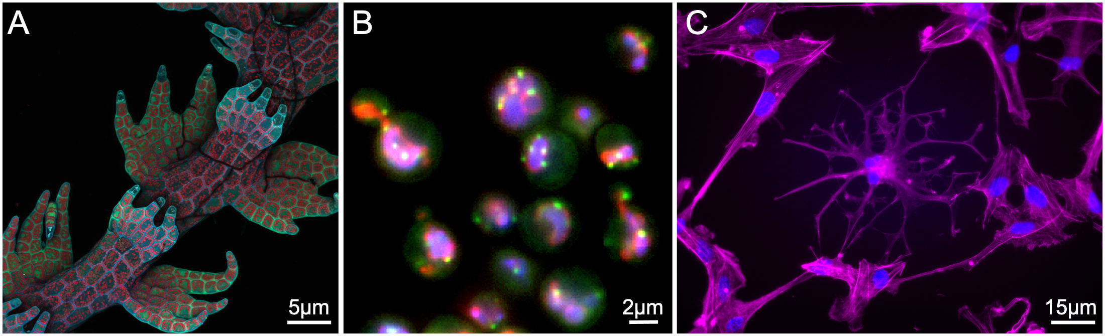
Fluorescence microscopy was first developed in the 1980s and has continued to revolutionize cell biology to this day. Not only does it allow us to view live samples, as other forms of light microscopy do, but it also allows us to label (or tag) specific macromolecules / cell structure so that we can track them within the cell (Figure 01-04B). We tag the structures using fluorescent molecules (called fluorochromes or fluorophores). Then, using our fluorescent microscope, we illuminate the sample with light of a particular wavelength, and the fluorophore responds by emitting light at a second known wavelength that we can then detect. The great advantage of this technique is that only the molecule or structure of interest shows up in the image, and the rest of the sample, which is not emitting light, is dark.

Much like transmitted light microscopy, there are several subtypes of fluorescent light microscopy. Most of these have been developed to increase the resolution of the images that are being viewed. The simplest type of fluorescence microscopy is known as epifluorescence, which uses powerful halogen lightbulbs and colored filters to produce light of specific wavelengths. Confocal laser scanning microscopy (or confocal for short) is very similar to epifluorescence, except a laser is used as the source of light. Using a laser allows us to focus the light very specifically and then use computer algorithms to remove out-of-focus light. There are also a number of extremely advanced techniques that allow us to seemingly “break” the laws of physics. Using a combination of computer algorithms and specific image collection protocols, microscopists have been able to resolve structures that should be much too small to see in light microscopy. These techniques are collectively known as superresolution microscopy.

Unlike the different kinds of transmitted light microscopy, the images that you create from the different subtypes of fluorescence light microscopy are very similar. It’s not always easy to tell what kind of fluorescence microscope was used to create the image just by looking at it. For this reason, we will not differentiate between the different types in this textbook. Instead, we will treat the images that are created using fluorescence microscopy as a single group. Examples of different fluorescence microscopy images are shown in Figure 01-06.

Sample Preparation for Fluorescence Microscopy

There are several approaches to sample preparation in fluorescence microscopy. It depends on both the scientific question you’re trying to answer and the fluorescent stains you have available. There are a number of chemical stains that can be added to live cells that latch onto specific components of the cell and then fluoresce. This is known as direct staining. An example of this is DAPI, which fluoresces when bound to double-stranded DNA. This is great when you’re interested in exploring a sample for which a fluorescent live-cell stain exists. Sadly, that is not always the case.

Another option is immunolabeling. In this case, antibodies bound to a fluorophore that have been specifically created to bind to your protein or structure of interest are used to label the cell. If your structure/molecule of interest is on the cell surface, then this works just fine. However, if your structure is in the interior of the cell, then the antibody will have difficulty accessing it. In this case, the cell is usually treated with fixatives, which kill it but also hold everything in place. Then the membrane can be disrupted just enough to allow the antibodies to access the interior of the cell.

One of the most important advances in fluorescence microscopy was the development of genetic engineering protocols so that one could add a fluorescent tag to any protein in the cell. There are a number of naturally occurring proteins that fluoresce and are used by organisms to produce bioluminescence. Some of the fluorescent proteins have been isolated and attached to other, nonfluorescent proteins. The most commonly used tag is known as green fluorescent protein (GFP), which was isolated from bioluminescent jellyfish. As its name states, GFP is a protein that fluoresces in the green range of visible light (~550 nm) when it is illuminated with blue light (~450 nm). The genetically engineered protein usually functions like the normal protein, except it now fluoresces its location under a particular wavelength of light. Thus, we can now track structures that include the fluorescent protein.

GFP was first isolated in the 1980s, but since then, we have genetically modified it to create versions in virtually every wavelength of the visible spectrum. We’ve even been able to produce forms that are split in half and only fluoresce when the two halves come together so as to identify when two proteins of interest interact with each other.

Topic 1.3: Electron Microscopy

Electron microscopy works in a very similar way to light microscopy, except that it uses a beam of electrons instead of light to image the sample. Since electrons can easily be scattered by air molecules (which would destroy our ability to use them for imaging), almost all electron microscopy is done in a vacuum, including both transmission electron microscopy (TEM) and scanning electron microscopy (SEM). The “electron gun” is the source of electrons. Electricity is sent through a metal filament (often made of tungsten) until it releases electrons into the vacuum of the microscope. Electromagnetic lenses (similar in function to the optical lenses of the light microscope) are used to control and focus the electron beam so that the sample can be imaged.

Again, like both brightfield and fluorescence microscopy, there are several types of electron microscopy that exist—more than we can reasonably discuss here. Here we focus on the two types that are most commonly used to study biological materials.

Resolution

Electrons have shorter wavelengths than photons in the visible light spectrum. For the electron microscope, an accelerating voltage of 100 kV produces a beam wavelength of close to 0.004 nm. The numerical aperture of the instrument is close to 0.012, so take a minute and calculate the resolution of the electron microscope using the equation from earlier in this chapter. (Hint: It’s 0.2 nm.) That’s a 1,000× smaller resolution than we calculated for the light microscopes.

Each of these types of electron microscopy functions quite differently, so we must also look at each one in more detail as well.

Transmission Electron Microscopy (TEM)

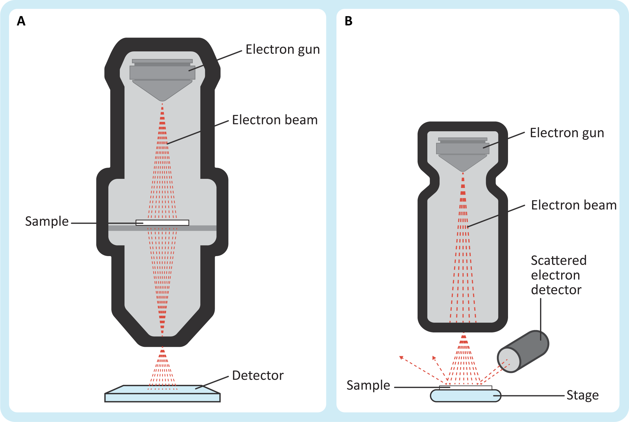
In many ways, TEM is analogous to traditional brightfield light microscopy, but with much greater capabilities with respect to magnification and resolution. The sample sits between the electron source and the detector (Figure 01-08A) so that the beam of electrons passes through the sample on its way to the detector. Just like in brightfield light micrographs, the empty spaces will show up as white in the image. Unlike light microscopy, there is no color in electron micrographs. Instead, the areas where the electrons were absorbed by the sample will be gray or black (depending on how “electron dense” your sample is in that region).

In TEM, the electron beam passes through the specimen. Electrons cannot penetrate very deeply, so the specimen must be extremely thin. The specimens are typically 50–100 nm sections of cells that have first been stained with heavy metals and then embedded in plastic resin. As you can imagine, all of this sample processing, along with the fact that the inside of a TEM is a vacuum, means that TEM cannot be used with living material. Instead, samples are carefully preserved, prior to embedding in epoxy resins, by either flash freezing (also known as cryofixation) or using chemical fixatives. If we do this carefully enough, we can capture cellular events that were happening at the moment of fixation. Being gentle with samples so as to avoid disturbing the location of each and every molecule while also removing water and replacing it with epoxy resin is very difficult, which is why this process can take days, weeks, or even months.

The electrons that have passed through the specimen are collected by an electron detector attached to a digital camera. An example is shown in Figure 01-08, where some of the subcellular structures in a plant cell have been labeled for you.

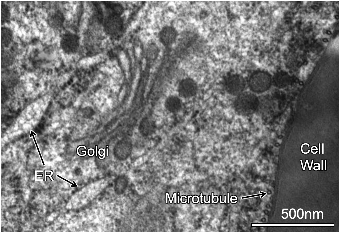
Much like in light microscopy, samples must be stained so that the structures are visible. As mentioned, we use heavy metal stains for electron microscopy. This is because of how electrons are able to move in heavy metal atoms. Heavy metals like lead (Pb), uranium (U), osmium (Os), gold (Au), and silver (Ag) are considered to be more “electron dense” and thus will be better able to block the electron beam than the atoms biological samples are made of, primarily carbon (C), oxygen (O), and hydrogen (H). We are also able to use immunolabeling in TEM in order to identify the location of specific proteins. However, we use colloidal gold particles of a specific size, rather than any kind of fluorescent tag, that are attached to antibodies that recognize our structure or protein of interest.

Negative staining is another technique that is most commonly used to examine very small objects, such as bacteria, viruses, and even individual proteins. In this technique the sample is suspended in an electron-dense stain that does not penetrate the sample but rather surrounds it so that it is outlined and all of the cracks and crevices can be observed.

Scanning Electron Microscopy (SEM)

In SEM, the specimen is usually dried and coated with a very thin layer of gold, platinum, or another heavy metal. The electron beam is “scanned” across the surface of the specimen. As the beam of electrons hits the specimen, secondary electrons are scattered from the surface of the specimen (Figure 01-08B). These are collected by a detector that builds an image electronically based on electron intensity (from white to black). This technique produces images of surfaces only. Since this microscope also uses electrons to image, the magnification and resolution are similar to TEM.

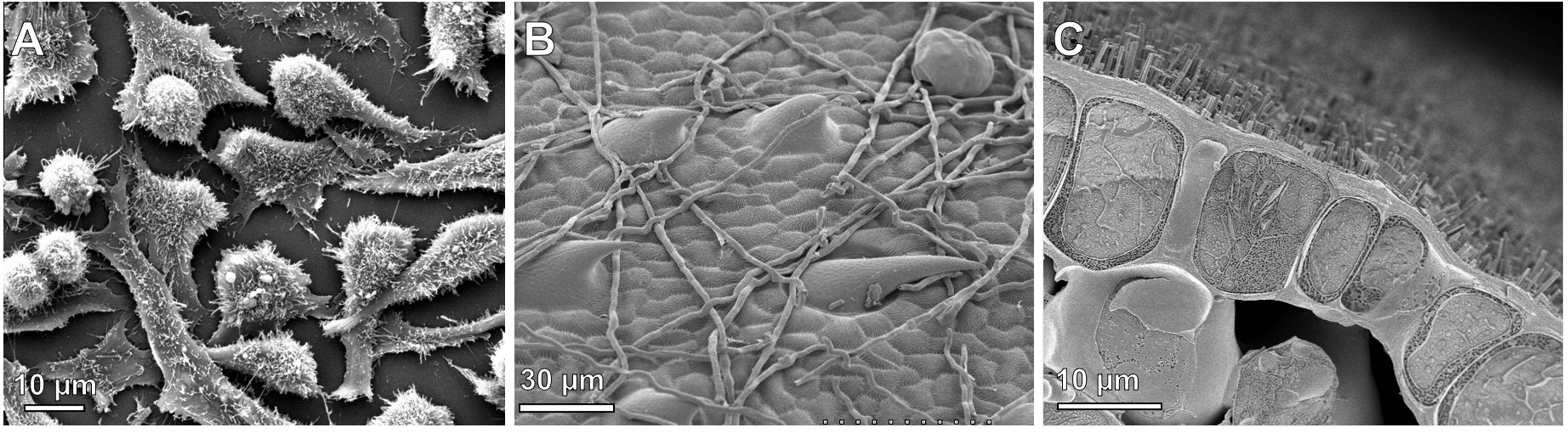
While samples are usually dead, when imaged with SEM, they do not have to be embedded in plastic like they are for TEM. Panels B and C of Figure 01-09 are of material that was cryofixed and imaged in the frozen state.

Topic 1.4: Putting It into Practice: Determining the Type of Microscopy from the Micrograph

One of the major skills you should be practicing as you learn about cell biology is how to interpret micrographs. This is not a trivial skill to learn. However, the very first step in this process is being able to identify the type of microscopy that was used based solely on the image.

When you look at a micrograph of any kind, there are a number of questions that you should be asking yourself, including the following:

• What is the magnification/scale of the image? Can I find a scale bar or other information to help me tell?
• Does the image look three-dimensional? Is there depth to the image?
• Is there a black background? Does the sample look like only some of the structures in the sample are visible?
• What types of structures do I think I can see? Does that match with the magnification/resolution I would expect based on the type of microscopy?
• Is it in color? Does the color look like it might be computer-generated after the fact?
• Is it moving? Does it look like it could have been imaged live?
• Finally, what other information do I have about this image? Is there a figure legend or other text associated with the image that provides insight? It is quite common to place additional information in the text associated with the image, as we have done in this textbook chapter. Any information that you have about an image is there for you to use, so don’t forget to use it!

There is no single question in this list that can determine definitively what kind of microscopy was used. However, a combination of answers could help you make a reasonable decision, or at least a solid guess, based on the evidence. And every time you look at a new image, you’re going to have to figure it out again.

Light versus Electron Microscopy and the Question of Scale

While the size of what you’re looking at can be an important indicator of what type of microscopy you’re looking at, it’s also important to realize that more than one type of microscopy can often be used at any given magnification. We have repeated Figure 01-02 below because it does such a good job of visualizing the overlap and also to facilitate the discussion we’re about to have. It’s important to know what you can reasonably see in each type of microscopy so that you can make appropriate predictions about the information within the micrographs that you’re interpreting.

It is common when learning to identify microscopy from images to assume that anything imaged at a lower magnification is taken with a light microscope and anything at a higher magnification must be electron microscopy. However, that is not necessarily the case. Notice in Figure 01-02 that there is quite a lot of overlap in the range of light and electron microscopy. Other than the most extreme ends of very low magnification (like whole tissues, with many cells visible) and very high magnifications (like individual ribosomes), either type of microscopy can be used. This means that you need to take into consideration more than just the magnification. As we mentioned at the beginning of this chapter, resolution is also extremely important. For example,

• If you are using a light microscope at very high magnifications, you may be able to see bacteria (like E. coli as shown in the figure), but you won’t be able to see much of the details of the cytosol.
• On the other hand, at the same magnification, an electron microscope would likely allow you to see much more fine detail. You would likely be able to identify the location of the nucleoid and see some of the details of the flagella and their attachment to the plasma membrane.

Brightfield versus Transmission Electron Microscopy (TEM)

We have also found that it can be quite challenging for students to differentiate between a lower-magnification TEM image and a higher-magnification brightfield image. Video 01-01, posted earlier in this chapter, does an excellent job of explaining this, so we would encourage you to watch that video if you haven’t already. However, here are some things to consider that might help you to tell the difference:

• Brightfield microscopy allows for much lower magnification images than TEM does. At best, a low-magnification TEM image would only allow you to see two or three cells, so if you can see more than that, it’s probably brightfield.
• Similarly, TEM allows for much higher magnification images, so if you’re seeing only a small subsection of the cell’s cytoplasm in great detail, it’s probably TEM.
• If you can see a whole cell, or even a large part of a cell, it could be either TEM or brightfield, so here you need to think about resolution. TEM will show much more of the finer details of the cytoplasm, and many of the organelles will likely be identifiable. Brightfield is more likely to show you a bunch of fuzzy blobs inside the cell, and you may not be able to tell what they all are.
• Any technique that uses light microscopy has the potential to produce color images, so that could be something to consider as well, but cautiously. Remember that color is exceptionally easy to manipulate in digital images, and it can be added and removed at will. Also, if you are working to identify micrographs on a paper exam, it will most likely be printed in black and white, so you may or may not have the information about color in the image you are analyzing.

Scanning Electron Microscopy (SEM) versus Fluorescence Microscopy

With the advances in fluorescence microscopy and the ability to digitally reconstruct a stack of images into a single 3D image, it can also be challenging to tell the difference between images created by these two types of microscopes.

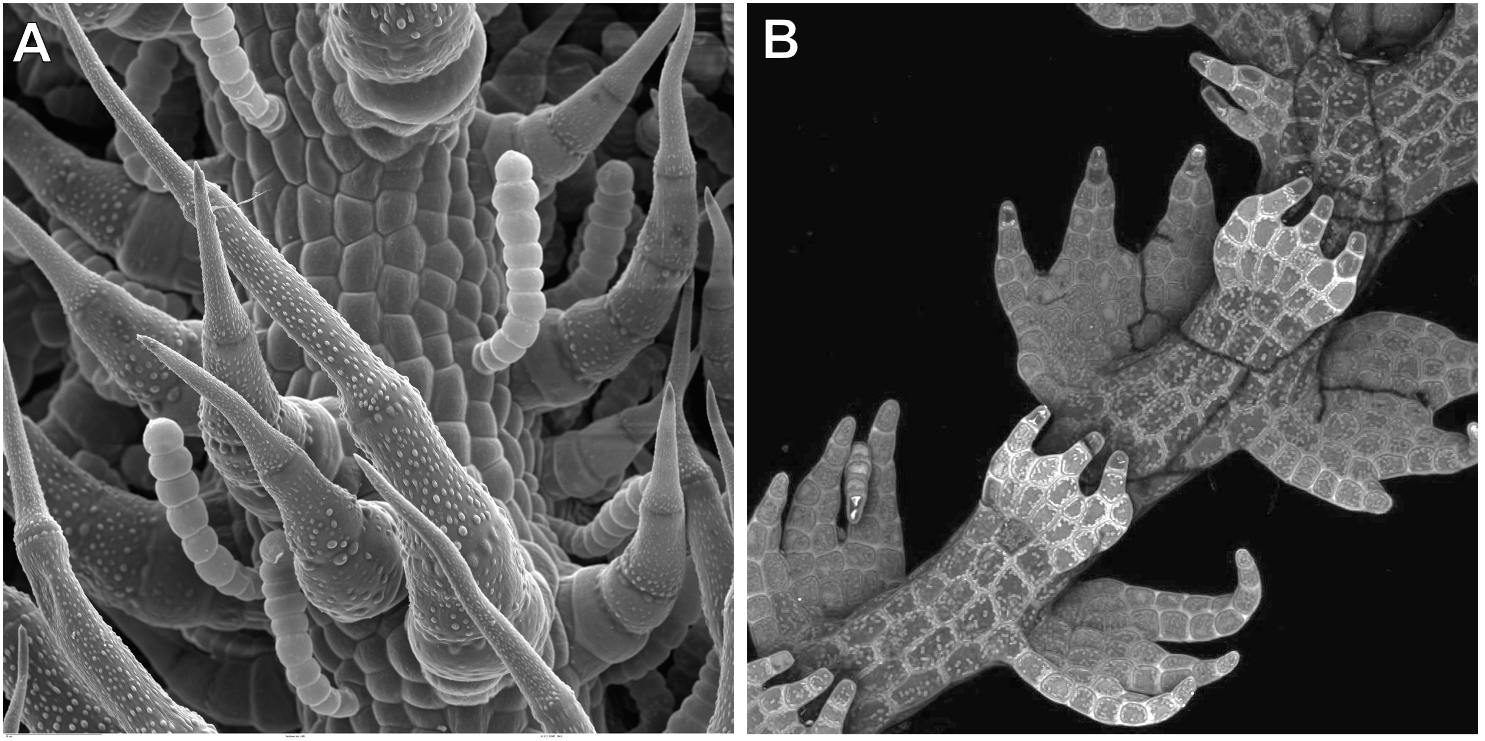
The key difference is that in SEM, you can only ever see the surface of the sample. (Compare Panels A and B from Figure 01-10.) In Figure 01-10A, we have an SEM image, which shows the surface structure of a leaf. Only the surface of the leaf cells is visible and nothing else. On the other hand, in fluorescence microscopy, the sample itself is emitting the light that you are viewing. This means that anything that is emitting light will be visible, whether it’s an internal structure or a surface element. In Figure 01-12B, it looks as if the cells are little compartments with dots in them. The dots are the chloroplasts inside the cell, emitting light. So even though this image looks 3D, we can still see beyond the surface of the sample, into the interior of the cells. Sometimes in SEM, the tissue is cracked open, so the inside of the cells is visible. (See Figure 01-12C for an example.) However, it is still very clear that it is the surface of the sample that’s being viewed in SEM, even though that surface is from the interior of the cell.

One additional thing to look for is the “quality” of the blackness of the background (when visible). In fluorescence, since the light is being emitted by the sample, the background will be very black, with no defining features. In SEM, however, the electrons are bounced off the surface of the sample, so there’s more likely to be some depth or texture to the background, even when it’s very dark/black. This may be subtle, but when visible it gives a useful clue.

Of course, none of these tricks work 100% of the time. The technology we have developed for imaging is very good, and the differences between them are getting smaller. There are times when it can be impossible to tell. In those cases, there are still options. In these cases, we encourage you to take your best guess based on the evidence you have. Sometimes that is all you can really do, and then you can see where the rest of the conversation takes you.

Microscopes are arguably the most essential tool to study cell biology. Virtually everything we study in cell biology is far too small to see with the naked eye. There have been some pretty significant advances in microscope technology, especially in the last 100 years. Here we break down the different forms of microscopy into the following:

1. emitted light microscopy, represented by the brightfield light microscope
2. transmitted light microscopy, represented by the fluorescent light microscope
3. transmission electron microscopy (TEM)
4. scanning electron microscopy (SEM)

Each one has different capacities in terms of magnification and resolution, both of which are key to determining what you should expect to see with each of these microscopes. It’s important to remember that the bulk of cell biology is within a size range that allows both light and electron microscopy to be used, so it’s important to consider how much detail you can see (i.e., the resolution), as well as the magnification and other parameters, when trying to decide how a sample was imaged.