23 Uncertainty and Risk

The Policy Question
Should the US Government Provide Flood Insurance?

Much insurance is provided by the private market, but one important exception is flood insurance, which is generally provided by the federal government in the United States. The country’s National Flood Insurance Program is run by the Federal Emergency Management Agency and provides supplemental flood insurance for flood-prone homes, as most private homeowner policies do not cover flood damage.

Exploring the Policy Question

1. Why don’t private insurers provide flood insurance?
2. What is the justification for government provision of flood insurance?

23.1 What Are Risky Outcomes?

Learning Objective 23.1: Define risky outcomes, and describe how they are assessed.

Risk describes any economic activity in which there are uncertain outcomes. For example, a person who places a bet on the flip of a coin faces two different outcomes with equal chance. A driver of a car knows that there is a chance of a collision. People understand that in the future, there is a possibility that they will fall ill or suffer an injury that requires medical attention. All of these scenarios are examples of uncertainty, and uncertainty implies risk. For this chapter, as in economics in general, we use the terms risk and uncertainty interchangeably.

Associated with any uncertain outcome are probabilities. Recall that probabilities are numbers between zero and one that indicate the likelihood that a particular outcome will occur. In a coin flip, the probability of one side landing facing up is one-half, or 50 percent. Sometimes these probabilities are known, like in the coin-flipping example, and sometimes these probabilities are unknown, like in the car-collision example. Even when we don’t know the probabilities, we can often estimate based on aggregate data or some other information, such as if the roads are covered in snow. In either case, the ability to assign probabilities distinguishes these risks as quantifiable. We will only consider quantifiable risk in this chapter.

In the absence of a known probability like a coin flip, economic agents have to estimate. They generally do so in two ways: they can estimate based on frequency or based on subjective probability. Frequency is how often a particular outcome has occurred over a known number of events. For example, a person who lives in an area that only rarely gets snow in the winter might wonder what the chances are that there will be snow this winter. They might remember that in the last ten years, it has snowed in three of them. Therefore, they might estimate the probability of snow this year based on its annual frequency, 3/10, or .3, or 30 percent. Formally, if [latex]k[/latex] equals the number of times an event has occurred and [latex]N[/latex] equals the number of times possible, then the frequency, [latex]F[/latex], equals

[latex]F=\frac{k}{N}[/latex].

Subjective probability is when individuals estimate probabilities based on their own experiences and whatever data are available to them. For example, a homeowner might not have ever experienced a house fire but might make an inference about how likely they are based on their own knowledge of fires in their community and reports of fires they see in the news. A weather forecaster is also making a subjective probability estimate when forecasting a chance of rain. They look at the data and models available to them but use their own experience as a guide on how to interpret the data and model predictions and make their own assessments.

If there are multiple possible outcomes, probabilities can be assigned to each one. The expected value of an uncertain outcome is the sum of the value of each possible outcome multiplied by the probability it will occur. For example, consider a jar of one hundred marbles of four different colors: red, blue, green, and yellow. If there are forty red marbles, twenty blue marbles, thirty green marbles, and ten yellow marbles, then the probability of randomly drawing a red one is .4 (40/100), a blue one is .2, a green one is .3, and a yellow one is .1. Suppose also that red ones are worth $10, blues ones are worth $50, green are worth $20, and yellow are worth $100. The expected value (EV) of one random draw is

[latex]EV = Pr(Red) \times Value(Red) + Pr(Blue) \times Value(Blue)[/latex]
[latex]+ Pr(Green) \times Value(Green) + Pr(Yellow) \times Value(Yellow)[/latex]

or

[latex]EV =.4 \times $10 + .2 \times $50 + .3 \times $20 + .1 \times $100 = $30[/latex].

The expected value from the marble game is the amount one could expect to earn on average if the game is repeated many times. The average outcome of the marble game is to earn $30.

23.2 Evaluating Risky Outcomes

Learning Objective 23.2: Explain expected utility and risk preference.

Consider the following gamble. With an 80 percent chance, you will win $400, and with a 20 percent chance, you will win $2,500. The expected value of this gamble is [latex]EV = .6 \times $1,000 + .4 \times $2,500 = $1,600[/latex]. A fair gamble is one where the cost of the gamble is equal to the expected value. But how much would you be willing to pay to play this game? In order to answer that, we need to know about expected utility.

Expected utility [latex](EU)[/latex] is the probability-weighted average utility a person gets from each possible outcome of an uncertain situation. To understand this concept, we can apply it to the gamble. The expected utility from the above gamble is

[latex]EU = .6 \times U($1,000) + .4 \times U($2,500)[/latex].

To look at a specific example, suppose a person’s utility can be expressed as a function of money in the following way:

[latex]U(Money)=\sqrt{Money}[/latex]

Then the expected utility from the above gamble is

[latex]EU=.6 × \sqrt{1,000}+.4x \sqrt{2,500}=.6x31.62+.2x50 \approx 29[/latex].

As with utility in general, this number does not mean anything in absolute terms, only as a relative measure. If instead this person were given the expected value of the gamble, $1,600, for certain, they would get

[latex]Y(\$1,600)=\sqrt{1,600}=40[/latex].

In other words, the guaranteed amount of $1,600 yields higher utility than the gamble that has an expected value of $1,600. This shows that the individual is risk averse.

A person who is unwilling to make a fair gamble, like the person above, is risk averse. A person who prefers the gamble to the guaranteed fair payout is risk loving. A person who is indifferent between the gamble and the fair payout is risk neutral.

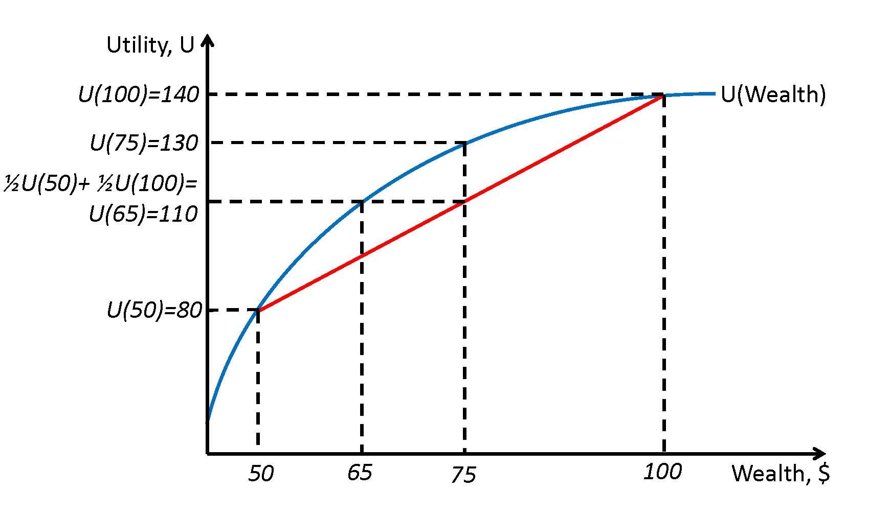
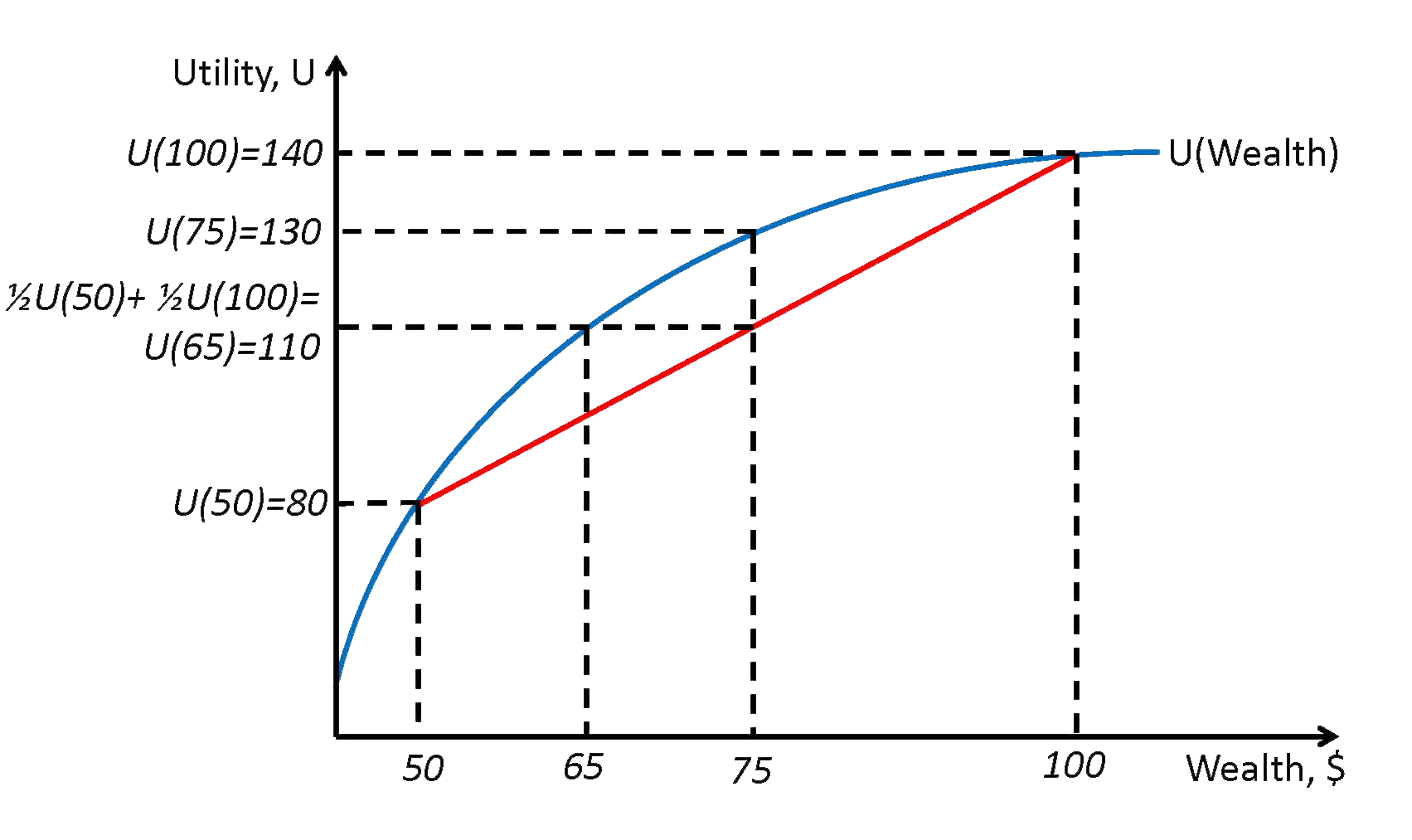
Figure 23.1 illustrates a person with a utility function with regard to wealth that is risk averse. The graph of the utility function has a declining slope as wealth increases. Consider two possible outcomes, $50 and $100. The graph tells us that the utility of $50 for this agent is 80 and the utility for $100 is 140. Remember that the value of the utility has no meaning in absolute terms, only in relative terms. So this agent prefers more wealth to less, but the marginal utility of wealth is decreasing. It is precisely this diminishing marginal utility of wealth that leads to risk aversion.

Now consider a game where a coin is flipped and the actual payment, $50 or $100, depends on which side of the coin is showing after the flip. This means that the agent has a 50 percent chance of getting $50 and a 50 percent chance of getting $100. In expected value, the game is worth $75. The utility of $75 for this agent is 130, as shown in the figure. The expected utility is the average of the utility levels at the two outcomes and can be seen as the midway point on the chord that connects the two points on the utility function. Expected utility is [latex](.5)(80)+(.5)(140)=110[/latex]. This means that playing this risky game yields a utility of 110 for this agent.

What certain payment would yield the agent the same utility? If we look at the figure, we see that point d on the graph of the utility function is at $65. The difference between the expected value of the gamble, $75, and the amount of the certain payment that yields the same utility as the gamble, $65, is called the risk premium. In this case, the risk premium is $10. The risk premium is the amount an agent is willing to pay to avoid the risk of a fair gamble.

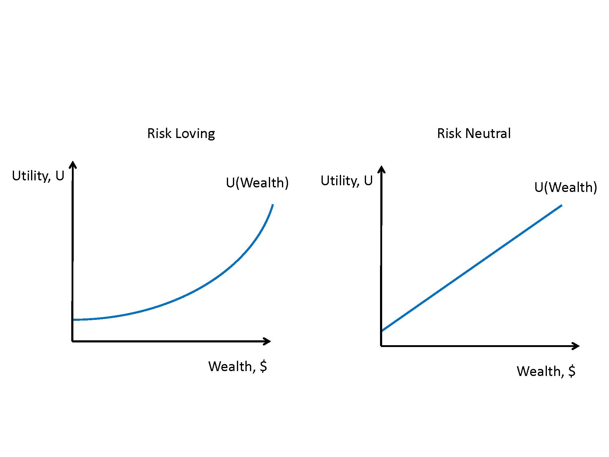
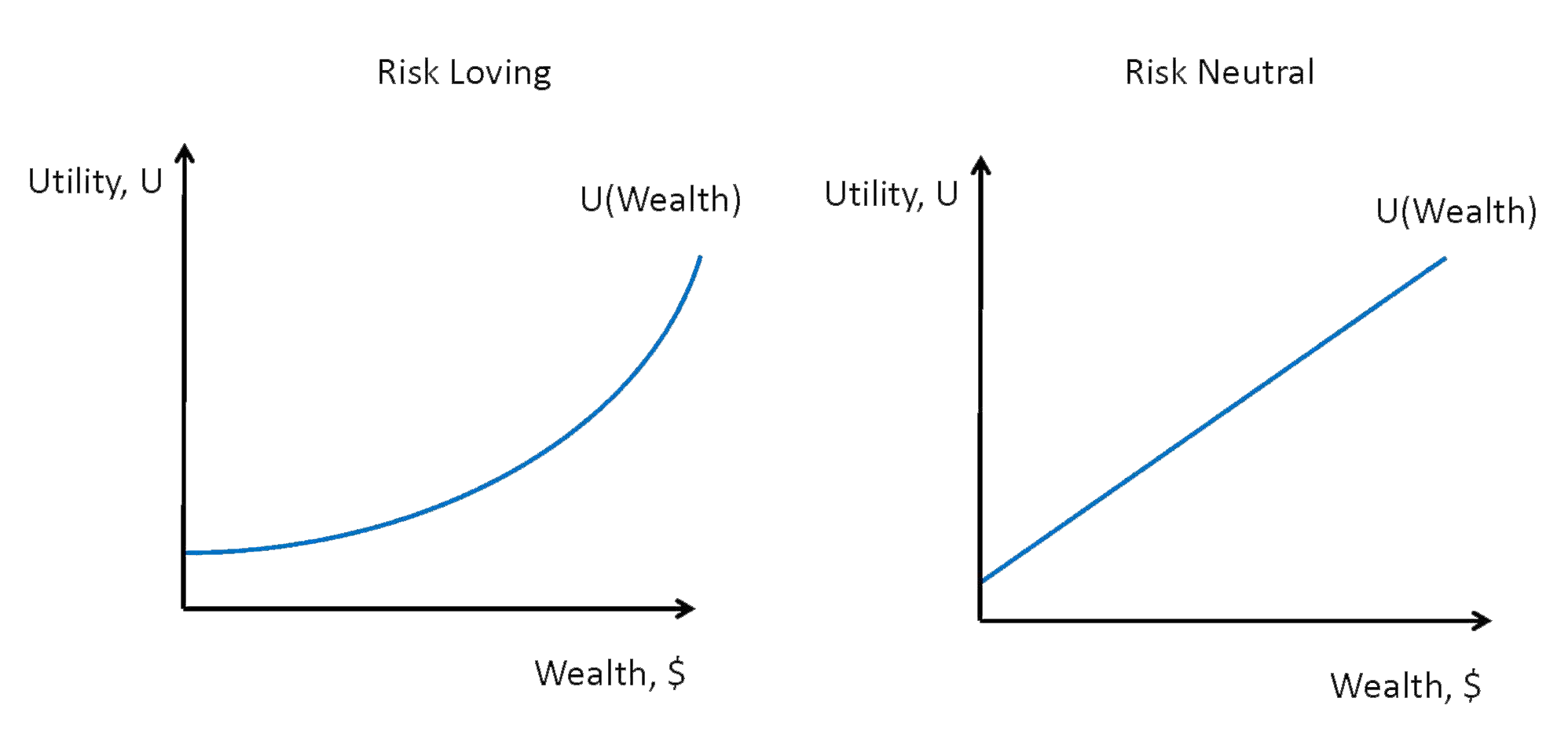
Graph of Risk-Neutral and Risk-Loving Utility Curve

Not all individuals are risk averse. An individual with a constant marginal utility of wealth is risk neutral, and an individual with an increasing marginal utility of wealth is risk loving. Figure 23.2 illustrates both situations, using the same scenario as in figure 23.1. Note that there is no risk premium for the risk-neutral individual, and the risk-loving individual would actually suffer a cost if the gamble were removed.

23.3 Risk Reduction

Learning Objective 23.3: Describe how diversification and insurance mitigate risk.

Risk-averse individuals wish to diminish or eliminate entirely the risks they face. Even risk-neutral individuals avoid unfair risks, and risk-loving individuals may wish to avoid very unfair risks. The easiest way to avoid risk is to abstain from risky activities, but it is not always possible to do so. A farmer, for example, cannot avoid the inherent variability of the weather. But there are some actions individuals can take to mitigate risk: drivers can drive more carefully, farmers can plant drought-resistant crops, and travelers can avoid airlines with poor safety records. Often, the ability to mitigate risk through conscious choices requires information about the risks. For example, in order to lower risk from air travel, a traveler would need access to the safety records of airlines.

Another way to reduce risk is through diversification. In a simple example, a farmer might plant some crops that grow well in dry conditions and others that grow well in wet conditions so that no matter if it is a wet or a dry year, the farmer will have at least one good harvest. This diversification requires that the risks are perfectly negatively correlated. Risks that are negatively correlated in general can be combined to reduce overall risk. For example, consider investing in the stock market. Investing in a few firms in the same industry is risky because their risks are probably positively correlated. If one firm in the automotive industry is doing poorly, it might be because demand for cars is soft and thus all automobile manufacturers might be doing poorly as a result. However, if you invest in many firms across a wide range of industries, it is likely that some will do well, while others will do poorly, and therefore the overall risk will be reduced.

A common way that individuals reduce risk is through the purchase of insurance. Private insurance markets exist thanks to the risk premium described earlier in the chapter. Risk-averse individuals are willing to pay a price to avoid or lower risk. Risk-averse individuals will always choose to purchase fair insurance. Fair insurance is a contract that has an expected value to the insurer as zero—in other words, a fair bet. As a simple example, consider an auto insurance policy. Suppose there is a 1 percent chance a driver will have an accident in a year. If an accident occurs, the cost of the damage will be $5,000. Thus the expected loss is (.1)($5,000), or $50. A fair insurance contract is one that would fully insure against this loss and charge the driver exactly the expected cost, or $50. This contract offers no profit for the insurance company, however. In fact, a risk-averse individual would be willing to buy insurance that is less than completely fair due to the risk premium, which gives rise to the private insurance industry.

The private insurance industry relies on diversified risk in order to stay in business. If an insurer has one thousand clients, each with a 1 percent risk of needing to make a claim, it is necessary that the 1 percent risk is not too positively correlated to avoid situations in which too many insured make claims in the same year. The insurance company relies on the fact that it can expect, on average, ten claims a year to keep its business going and not suffer a catastrophic loss from too many insured filing claims in the same year, which could bankrupt them. Take mortgage insurance, for example. Insurers will cover the loss to banks if a homeowner with a mortgage defaults. Normally, these risks are quite diverse, particularly if the insurer insures mortgages across a diverse geographical area so that an economic downturn in one city, like the closure of a large employer, will not cause too many claims at one time. This is normally a safe strategy, but the 2006 housing crisis in the United States spread across the entire country and led to a number of mortgage insurers falling into deep crises, most notably American International Group (AIG), which was bailed out by the US government to the tune of $180 billion dollars and led to the government taking control of the firm.

23.4 The Policy Question
Should the US Government Provide Flood Insurance?

Learning Objective 23.4: Apply knowledge of risk and insurance to explain how systematic risk makes risk pools difficult and destroys private markets for insurance.

Risk-averse homeowners whose houses are situated in areas that have a possibility of flooding will have a demand for insurance as long as the insurance contract is within the risk premium the homeowners are willing to pay. But flood insurance is not easy to acquire on the private market. The reason for this is the fact that most people who wish to purchase flood insurance own homes in flood-prone areas. Floods are relatively uncommon but very costly. When a flood happens, most homes in the flood area are severely damaged, so the risks are highly and positively correlated. This makes insuring against floods very difficult for private insurers who struggle to diversify their risk portfolio and puts them in danger of a catastrophic payout should a flood occur. For this reason, much of private insurance is priced beyond the risk premium of private homeowners. This is exacerbated by the fact that it is common that homeowners in flood-prone areas are disproportionately low-income households because flood-prone land is generally cheaper than land in higher areas. Lower-income households have more limited resources with which to deal with the costs of a flood should they not have insurance.

For these reasons, the federal government has stepped into the flood insurance market and provides subsidized insurance for flood-prone households. The federal government has the resources to deal with correlated risks and expensive payouts that most private insurers do not.

Learn: Key Topics

Terms

Probabilities

Probabilities are numbers between zero and one that indicate the likelihood that a particular outcome will occur. Subjective probability is when individuals estimate probabilities based on their own experiences and whatever data are available to them.

Frequency

Frequency is how often a particular outcome has occurred over a known number of events.

Expected value

The expected value of an uncertain outcome is the sum of the value of each possible outcome multiplied by the probability it will occur.

Fair gamble

A fair gamble is one where the cost of the gamble is equal to the expected value.

Expected utility

Expected utility is the probability-weighted average utility a person gets from each possible outcome of an uncertain situation.

Risk averse

A person who is unwilling to make a fair gamble, like the person above, is risk averse.

Risk loving

A person who prefers the gamble to the guaranteed fair payout is risk loving.

Risk neutral

A person who is indifferent between the gamble and the fair payout is risk neutral.

Risk premium

The difference between the expected value of the gamble and the amount of the certain payment that yields the same utility as the gamble is called the risk premium.

Graphs

Graph of risk aversion

Risk-loving and risk-neutral utility curves