18 Models of Oligopoly: Cournot, Bertrand, and Stackelberg
Cournot, Bertrand, and Stackelberg
The Policy Question
How Should the Government Have Responded to Big Oil Company Mergers?
Exploring the Policy Question
- How do oil companies compete—on quantities or prices?
- What policy solutions present themselves from this analysis?
Learning Objectives
18.1 Cournot Model of Oligopoly: Quantity Setters
Learning Objective 18.1: Describe how oligopolist firms that choose quantities can be modeled using game theory.
18.2 Bertrand Model of Oligopoly: Price Setters
Learning Objective 18.2: Describe how oligopolist firms that choose prices can be modeled using game theory.
18.3 Stackelberg Model of Oligopoly: First-Mover Advantage
Learning Objective 18.3: Describe the different outcomes when oligopolist firms choose quantities sequentially.
18.4 Policy Example
How Should the Government Have Responded to Big Oil Company Mergers?
Learning Objective 18.4: Explain how models of oligopoly can help us understand how to respond to proposed mergers of oil companies that sell retail gas.
18.1 Cournot Model of Oligopoly: Quantity Setters
Learning Objective 18.1: Describe how oligopolist firms that choose quantities can be modeled using game theory.
Oligopoly markets are markets in which only a few firms compete, where firms produce homogeneous or differentiated products, and where barriers to entry exist that may be natural or constructed. There are three main models of oligopoly markets, and each is considered a slightly different competitive environment. The Cournot model considers firms that make an identical product and make output decisions simultaneously. The Bertrand model considers firms that make an identical product but compete on price and make their pricing decisions simultaneously. The Stackelberg model considers quantity-setting firms with an identical product that make output decisions simultaneously. This chapter considers all three in order, beginning with the Cournot model.
| Number of firms | Similarity of goods | Barriers to entry or exit | Chapter | |
|---|---|---|---|---|
| Perfect competition | Many | Identical | No | 13 |
| Monopolistic competition | Many | Distinct | No | 19 |
| Oligopoly | Few | Identical or distinct | Yes | 18 |
| Monopoly | One | Unique | Yes | 15 |
Oligopolists face downward-sloping demand curves, which means that price is a function of the total quantity produced, which, in turn, implies that one firm’s output affects not only the price it receives for its output but the price its competitors receive as well. This creates a strategic environment where one firm’s profit maximizing output level is a function of its competitors’ output levels. The model we use to analyze this is one first introduced by French economist and mathematician Antoine Augustin Cournot in 1838. Interestingly, the solution to the Cournot model is the same as the more general Nash equilibrium concept introduced by John Nash in 1949 and the one used to solve for equilibrium in non-cooperative games in chapter 17.
We will start by considering the simplest situation: two companies that make an identical product and that have the same cost function. Later we will explore what happens when we relax those assumptions and allow more firms, differentiated products, and different cost functions.
Let’s begin by considering a situation where there are two oil refineries located in the Denver, Colorado, area that are the only two providers of gasoline for the Rocky Mountain regional wholesale market. We’ll call them Federal Gas and National Gas. The gas they produce is identical, and they each decide independently—and without knowing the other’s choice—the quantity of gas to produce for the week at the beginning of each week. We will call Federal’s output choice [latex]q_F[/latex] and National’s output choice [latex]q_N[/latex], where [latex]q[/latex] represents liters of gasoline. The weekly demand for wholesale gas in the Rocky Mountain region is [latex]P=A—BQ[/latex], where [latex]Q[/latex] is the total quantity of gas supplied by the two firms, or [latex]Q=q_F+q_N[/latex]. Immediately, you can see the strategic component: the price they both receive for their gas is a function of each company’s output. We will assume that each liter of gas produced costs the company c, or that c is the marginal cost of producing a liter of gas for both companies and that there are no fixed costs.
With these assumptions in place, we can express Federal’s profit function:
[latex]\pi_F=P \times q_F—c \times q_F = q_F (P-c)[/latex]
Substituting the inverse demand curve, we arrive at the expression
[latex]\pi_F=q_F(A-BQ-c)[/latex].
Substituting [latex]Q=q_A+q_B[/latex] yields
[latex]\pi_F=q_F(A-B(q_F+q_N)-c)[/latex].
The expression for National is symmetric:
[latex]\pi_N=q_N(A-B(q_N+q_F)-c)[/latex]
Note that we have now described a game complete with players, Federal and National; strategies, [latex]q_F[/latex] and [latex]q_N[/latex]; and payoffs, [latex]\pi_F[/latex] and [latex]\pi_N[/latex]. Now the task is to search for the equilibrium of the game. To do so, we have to begin with a best response function. In this case, the best response is the firm’s profit maximizing output. This will depend on both the firm’s own output and the competing firm’s output.
We know from chapter 15 that the monopolists’ marginal revenue curve when facing an inverse demand curve [latex]P=A-BQ[/latex] is [latex]MR(q)=A-2Bq[/latex]. This duopolistic example shows that the firms’ marginal revenue curves include one extra term:
[latex]MR_F(q_F)=A-2Bq_F-Bq_N[/latex] and [latex]MR_N(q_N)=A-2Bq_N-Bq_F[/latex]
The profit maximizing rule tells us that to find the profit maximizing output, we must set the marginal revenue to the marginal cost and solve. Doing so yields
[latex]q^*_F=\frac{A-c}{2B}-\frac{1}{2}qN[/latex]
for Federal Gas and
[latex]q^*_N=\frac{A-c}{2B}-\frac{1}{2}qF[/latex]
for National Gas. These are the firms’ best response functions, their profit maximizing output levels given the output choice of their rivals.
Now that we know the best response functions, solving for equilibrium in the model is relatively straightforward. We can begin by graphing the best response functions. These graphical illustrations of the best response functions are called reaction curves. A Nash equilibrium is a correspondence of best response functions, which is the same as a crossing of the reaction curves.
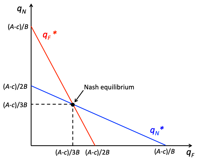
In figure 18.1, we can see the Nash equilibrium of the Cournot duopoly model as the intersection of the reaction curves. Mathematically, this intersection is found by simultaneously solving
[latex]q^*_F=\frac{A-c}{2B}-\frac{1}{2}q_N[/latex] and
[latex]q^*_F=\frac{A-c}{2B}-\frac{1}{2}q_F[/latex]
This is a system of two equations and two unknowns and therefore has a unique solution as long as the slopes are not equal. We can solve these by substituting one equation into the other, which yields a single equation with a single unknown:
[latex]q^*_F=\frac{A-c}{2B}-\frac{1}{2}[\frac{A-c}{2B}-\frac{1}{2}q_F][/latex]
Solving this by steps results in the following:
[latex]q^*_F=\frac{A-c}{2B}-\frac{A-c}{4B}+\frac{1}{4}q_F[/latex][latex]\frac{3}{4}q^*_F=\frac{A-c}{4B}[/latex]
[latex]q^*_F=\frac{A-c}{3B}[/latex]
And by symmetry, we know that the two optimal quantities are the same:
[latex]q^*_N=\frac{A-c}{3B}[/latex]
The Nash equilibrium is
[latex](q^*_F,q^*_N)[/latex]
or
[latex](\frac{A-c}{3B}, \frac{A-c}{3B})[/latex].
Let’s consider a specific example. Suppose in the above example, the weekly demand curve for wholesale gas in the Rocky Mountain region is
[latex]p = 1,000 − 2Q[/latex], in thousands of gallons
Both firms have constant marginal costs of 400. In this case,
[latex]A = 1,000[/latex], [latex]B = 2[/latex] and
[latex]C = 400[/latex].
So,
[latex]q^*_F=\frac{A-c}{3B}=\frac{1,000 − 400}{(3)(2)}=\frac{600}{6}=100[/latex]
By symmetry, we know
[latex]q^*_N=100[/latex]
as well. So both Federal Gas and National Gas produce 100,000 gallons of gasoline a week. Total output is the sum of the two and is 200,000 gallons. The price is [latex]p= 1,000 − 2(200) = $600[/latex] for 1,000 gallons of gas, or $0.60 a gallon.
To analyze this from the beginning, we can set up the total revenue function for Federal Gas:
[latex]TR(q_F)=p×q_F[/latex]
[latex]=(1,000 − 2Q)q_F[/latex]
[latex]=(1,000 − 2q_F-2q_N)q_F[/latex]
[latex]= 1,000 − 2q \frac{2}{F}-2q_Fq_N[/latex]
The marginal revenue function that is associated with this is
[latex]MR(q_F)=1,000 − 4q_F-2q_N[/latex].
We know marginal cost is 400, so setting marginal revenue equal to marginal cost results in the following expression:
[latex]1,000 − 4q_F-2q_N=400[/latex]
Solving for [latex]q_F[/latex] results in the following:
[latex]q_F=\frac{600 − 2q_N}{4}[/latex]
[latex]q^*_F=150-\frac{q_F}{2}[/latex]
This is the best response function for Federal Gas. By symmetry, we know that National Gas has the same best response function:
[latex]q^*_N=150-\frac{q_F}{2}[/latex]
Solving for the Nash equilibrium, we get the following:
[latex]q^*_N=150-\frac{q_F}{2}[/latex]
[latex]q^*_F=150 − 75+\frac{q_F}{4}[/latex]
[latex]/frac{3}{4}q^*_F=25[/latex]
[latex]q^*_F=100[/latex]
We can insert the solution for [latex]q_F[/latex] into [latex]q^*_N[/latex]:
[latex]q^*_N=150-\frac{(100)}{2}=100[/latex]
18.2 Bertrand Model of Oligopoly: Price Setters
Learning Objective 18.2: Describe how oligopolist firms that choose prices can be modeled using game theory.
In the previous section, we studied oligopolists that make an identical good and who compete by setting quantities. The example we used in that section was wholesale gasoline, where the market sets a price that equates supply and demand and the strategic decision of the refiners was how much oil to refine into gasoline. In this section, we turn our attention to a different situation in which the oligopolists compete on price. The example here is the retail gas stations that bought the wholesale gas from the refiners and are now ready to sell it to consumers. We still have identical goods; for consumers, the gas that goes into their cars is all the same, and we will assume away any other differences like cleaner stations or the presence of a mini-mart.
Let’s imagine a simple situation where there are two gas stations, Fast Gas and Speedy Gas, on either side of a busy main street. Both stations have large signs that display the gas prices that each station is offering for the day. Consumers are assumed to be indifferent about the gas or the stations, so they will go to the station that is offering the lower price. So an individual gas station’s demand is conditional on its relative price with the other station.
Formally, we can express this with the following demand function for Fast Gas:
[latex]Q_F \left\{\begin{matrix} & & & \\ a-bP_F \text{ if }P_F< P_S & & & \\ \frac{a-bP}{2} \text{ if }P_F=P_S & & & \\0 \text{ if }P_S> P_F \end{matrix}\right.[/latex]
Speedy Gas has an equivalent demand curve:
[latex]Q_S \left\{\begin{matrix} & & & \\ a-bP_S \text{ if }P_S< P_F & & & \\ \frac{a-bP}{2} \text{ if }P_S=P_F & & & \\0 \text{ if }P_S> P_F \end{matrix}\right.[/latex]
In other words, these demand curves say that if a station has a lower price than the other, they will get all the demand at that price, and the other station will get no demand. If they have the same price, then each will get one-half of the demand at that price.
Let’s assume that Fast Gas and Speedy Gas both have the same constant marginal cost of [latex]c[/latex] and no fixed costs to keep the analysis simple. The question we now have to answer is, What are the best response functions for the two stations? Remember that best response functions are one player’s optimal strategy choice given the strategy choice of the other player. So what is Fast Gas’s best response to Speedy Gas’s price?
If Speedy Gas charges
[latex]P_S \gt c[/latex]
Fast Gas can set [latex]P_F \gt P_S[/latex] and they will get no customers at all and make a profit of zero. Fast Gas could instead set
[latex]P_F=P_S[/latex]
and get [latex]\frac{1}{2}[/latex] the demand at that price and make a positive profit. Or they could set
[latex]P_F=P_S −$0.01[/latex]
or set their price one cent below Speedy Gas’s price and get all the customers at a price that is one cent below the price, at which they would get [latex]\frac{1}{2}[/latex] the demand.
Clearly, this third option is the one that yields the most profit. Now we just have to consider the case where [latex]P_S=c[/latex]. In this case, undercutting the price by one cent is not optimal because Fast Gas would get all the demand but would lose money on every gallon of gas sold, yielding negative profits. Setting
[latex]P_F=P_S=c[/latex]
would give them half the demand at a break-even price and would yield exactly zero profits.
The best response function we just described for Fast Gas is the same best response function for Speedy Gas. So where are the correspondences of best response functions? As long as the prices are above [latex]c[/latex], there is always an incentive for both stations to undercut each other’s price, so there is no equilibrium. But at [latex]P_F=P_S=c[/latex], both stations are playing their best response to each other simultaneously. So the unique Nash equilibrium to this game is
[latex]P_F=P_S=c[/latex].
What is particularly interesting about this is the fact that this is the same outcome that would have occurred if they were in a perfectly competitive market because competition would have driven prices down to marginal cost. So in a situation where competition is based on price and the good is relatively homogeneous, as few as two firms can drive the market to an efficient outcome.
18.3 Stackelberg Model of Oligopoly: First-Mover Advantage
Learning Objective 18.3: Describe the different outcomes when oligopolist firms choose quantities sequentially.
Both the Cournot model and the Bertrand model assume simultaneous move games. This makes sense when one firm has to make a strategic decision before knowing about the strategy choice of the other firm. But not all situations are like this. What happens when one firm makes its strategic decision first and the other firm chooses second? This is the situation described by the Stackelberg model, where the firms are quantity setters selling homogenous goods.
Let’s return to the example of two oil companies: Federal Gas and National Gas. The gas they produce is identical, but now they decide their output levels sequentially. We will assume that Federal Gas sets its output first, and then after observing Federal’s choice, National Gas decides on the quantity of gas they are going to produce for the week. We will again call Federal’s output choice [latex]q_F[/latex] and National’s output choice [latex]q_N[/latex], where [latex]q[/latex] represents liters of gasoline. The weekly demand for wholesale gas is still [latex]P = A—BQ[/latex], where [latex]Q[/latex] is the total quantity of gas supplied by the two firms, or
[latex]Q=q_F+q_N[/latex].
We have now turned the previous Cournot game into a sequential game, and the [latex]SPNE[/latex] solution to a sequential game is found through backward induction. So we have to start at the second move of the game: National’s output choice. When National makes this decision, Federal’s output choices are already made and known to National, so it is taken as given. Therefore, we can express Federal’s profit function as
[latex]\Pi _N=q_N(A-B(q_N+q_F)-c)[/latex].
This is the same as in the Cournot example, and for National, the best response function is also the same. This is because in the Cournot case, both firms took the other’s output as given.
[latex]q^*_N=\frac{A-c}{2B}-\frac{1}{2}q_F[/latex]
When it comes to Federal’s decision, we diverge from the Cournot model because instead of taking [latex]q_N[/latex] as a given, Federal knows exactly how National will respond because they know the best response function. Federal’s profit function,
[latex]\Pi _F=q_F(A-Bq_F-Bq_N-c)[/latex],
can be re-written, replacing [latex]q_N[/latex] with the best response function:
[latex]\Pi _F=q_F(A-Bq_F-B(\frac{A-C}{2B}-\frac{1}{2})-c)[/latex]
We can see that Federal’s profits are determined only by their own output once we explicitly consider National’s response. Simplifying yields
[latex]\Pi _F=q_F(\frac{A-c}{2}-B\frac{1}{2}q_F)[/latex].
We know that the second mover’s best response is the same as in section 18.1, and the solution to the profit optimization problem above yields the following best response function for Federal Gas:
[latex]q^*_F=\frac{A-c}{2B}[/latex],
substituting this into National’s best response function and solving the following:
[latex]q^*_N=\frac{A-c}{2B}-\frac{1}{2}\left [ \frac{A-c}{2B} \right ][/latex]
[latex]q^*_N=\frac{A-c}{2B}-\left [\frac{A-c}{4B} \right][/latex]
[latex]q^*_N=\frac{A-c}{4B}[/latex]
The subgame perfect Nash equilibrium is
([latex]q^*_F[/latex], [latex]q^*_F[/latex])
A few things are worth noting when comparing this outcome to the Nash equilibrium outcome of the Cournot game in section 18.1. First, the individual output level for Federal, the first mover in the Stackelberg game, the Stackelberg leader, is higher than it is in the Cournot game. Second, the individual output level for National, the second mover in the Stackelberg game, the Stackelberg follower, is lower than it is in the Cournot game. Third, the total output is larger in the Stackelberg outcome than in the Cournot outcome. This means the price is lower because the demand curve is downward sloping. Since the Cournot outcome is one of the options for the Stackelberg leader—if it chooses the same output as in the Cournot case, the follower will as well—it must be true that profits are higher for the Stackelberg leader. And since both the quantity produced and the price received are lower for the Stackelberg follower compared to the Cournot outcome, the profits must be lower as well.
So from this we see the major differences in the Stackelberg model compared to the Cournot model. There is a considerable first-mover advantage. By being able to set its quantity first, Federal Gas is able to gain a larger share of the market for itself, and even though it leads to a lower price, it makes up for that lower price with the increase in quantity to achieve higher profits. The opposite is true for the second mover: by being forced to choose after the leader has set its output, the follower is forced to accept a lower price and lower output. From the consumer’s perspective, the Stackelberg outcome is preferable because overall, there is more quantity at a lower price.
18.4 Policy Example
How Should the Government Have Responded to Big Oil Company Mergers?
Learning Objective 18.4: Explain how models of oligopoly can help us understand how to respond to proposed mergers of oil companies that sell retail gas.
The end of the twentieth century saw a number of mergers of massive oil companies. In 1999, BP Amoco acquired ARCO, followed soon thereafter by Exxon’s acquisition of Mobil. Then, in 2001, Chevron acquired Texaco for $38.7 billion. The newly combined company became the world’s fourth-largest producer of oil and natural gas. Whenever any such mergers and acquisitions are proposed, the US government has to approve the deal, and sometimes this approval comes with conditions designed to protect US consumers from undue harm that the consolidation might cause due to market concentration. In this case, the Federal Trade Commission (FTC) was the agency that provided oversight, and in the end, they approved the merger with the following condition: they had to sell their stake in two massive oil refineries. However, they were largely allowed to retain their retail gas operations, even though both companies had significant market presence and their merger would cause a drop in the competitiveness of the retail gas market, particularly in some areas where both companies had a significant market share.
On their face, these decisions seem to make little sense. How is it that the US government is worried about the impact of the merger on refining and the wholesale gas market but not on the retail gas market? The answer lies in the way these two markets fit into the economic models of oligopoly. Refining and wholesale gas operations are more akin to the Cournot model, where a few firms produce a homogenous product and compete on quantity and the sum total of all gas refined sets the wholesale market price. The insight of the Cournot model is that every merger produces fewer firms, and this constrains supply and increases price. Remember that this is a function not of capacity—that has not changed—but of the strategic environment, which makes it easier for all firms to constrict supply, which, in turn, raises prices and profits. The lower supply and higher prices do material harm to consumers, however, and it is for this reason that the FTC stepped in and demanded that the merged company sell off its interest in two big refining operations.
On the other hand, retail gas is more akin to the Bertrand model, where a bunch of retailers are selling a homogenous good but are competing mostly on price. A cursory examination of the retail gas industry confirms this: prices are posted prominently, and consumers show very strong responses to lower prices. The Bertrand model shows us that it takes very little competition to result in highly competitive pricing, so a merger that might reduce the number of competing gas station brands by one is unlikely to have much of a material effect on prices and therefore will be unlikely to harm consumers.
Viewed through the lens of the models of oligopoly studied in this chapter, the FTC’s decision to demand a divestment in oil refining and wholesale gas operations but mostly allow the retail side to consolidate makes sense. It is no surprise that these are the very same models the government uses to analyze such situations and devise a response.
Exploring the Policy Question
- Do you think it is correct that wholesale gas looks more like the Cournot model and retail gas looks more like the Bertrand model?
- Do you think the government did the right thing in the case of the Chevron-Texaco merger?
Review: Topics and Related Learning Outcomes
18.1 Cournot Model of Oligopoly: Quantity Setters
Learning Objective 18.1: Describe how oligopolist firms that choose quantities can be modeled using game theory.
18.2 Bertrand Model of Oligopoly: Price Setters
Learning Objective 18.2: Describe how oligopolist firms that choose prices can be modeled using game theory.
18.3 Stackelberg Model of Oligopoly: First-Mover Advantage
Learning Objective 18.3: Describe the different outcomes when oligopolist firms choose quantities sequentially.
18.4 Policy Example
How Should the Government Have Responded to Big Oil Company Mergers?
Learning Objective 18.4: Explain how models of oligopoly can help us understand how to respond to proposed mergers of oil companies that sell retail gas.
LEARN: KEY TOPICS
Terms
Oligopolist market
Oligopoly markets are markets in which only a few firms compete, where firms produce homogeneous or differentiated products, and where barriers to entry exist that may be natural or constructed.
The Cournot Model
The Cournot model considers firms that make an identical product and make output decisions simultaneously.
The Bertrand Model
The Bertrand model considers firms that make an identical product but compete on price and make their pricing decisions simultaneously.
The Stackelberg Model
The Stackelberg model considers quantity-setting firms with an identical product that make output decisions simultaneously.
Tables and Graphs
Metrics of the four basic market structures
| Number of firms | Similarity of goods | Barriers to entry or exit | Chapter | |
|---|---|---|---|---|
| Perfect competition | Many | Identical | No | 13 |
| Monopolistic competition | Many | Distinct | No | 19 |
| Oligopoly | Few | Identical or distinct | Yes | 18 |
| Monopoly | One | Unique | Yes | 15 |
Nash equilibrium in the Cournot duopoly model
Media Attributions
- 18.1.1 © Patrick M. Emerson is licensed under a CC BY-NC-SA (Attribution NonCommercial ShareAlike) license
