XI. Brief Introduction to CFD Basics
Why CFD
CFD (computational fluid dynamics) attempts to solve the basic (differential) conservation equations. These include the conservation of mass equation:
[latex]\frac{\partial \rho}{\partial t}+\nabla \cdot(\rho V)=0[/latex]
and the conservation of momentum equation:
[latex]\rho \frac{\partial V}{\partial t}+\rho(V \cdot \nabla) V=-\nabla p+\rho g+\nabla \cdot \tau_{i j}[/latex]
This set of equations are non-linear partial differential equations for unknowns of velocity and pressure. The stress tensor in the last term is represented in terms of the viscosity and strain rate tensor to arrive at the Navier-Stokes equations. The conservation of energy equation can be included as well for problems involving thermal effects. Compressible flow problems would also include density as a variable with a required equation of state. Unfortunately, an analytical solution for all but the most simple flows is, in general, not available. The alternative is an approximate solution using a discrete representation of these differential equations over a grid on points in space and time, the result is an algebraic set of equations that can be solved for the unknown variables.
CFD packages have been developed commercially and have grown to be very powerful, and widely used. Prior to their development extensive experimental efforts were needed, as well as using simplified models for practical solutions. Research continues to advance both CFD, as well as what are known as lower-order models, while trying to minimize the “computational cost”.
Since fluid mechanics is ubiquitous in a large number of applications, such as geophysical flows, biological and biomedical flow situations, chemical reactions and combustion situations, etc. CFD has becomes a powerful tool that can be used across many disciplines. Specific application of CFD is extensive, largely due to improved computing power allowing for greater accuracy and shorter times to obtain solutions. CFD is often used to simulate the flow in complex geometries. For instance, it can be used to study the steady and transient effects of moving surfaces (such as propellers, or control flaps on airplanes) as well as fuel and oxidizer inject into combustion chambers. It is also used for weather predictions, pollution analysis, ocean mixing, avalanche prediction, arterial blood flows, and a whole host of other areas.
In the solution to the Navier-Stokes Equations it is possible to identify the velocity field (over space and time) as well as the pressure distribution. These together allow the calculation of forces by integration of the local pressure at an object/fluid interface, as well as calculating the local wall shear stress and then integrating that over the interface as well. With the solution to the energy equation the temperature field and the local distribution of heat flux can be found.
An advantage of CFD when compared with experimental alternatives is the ability to readily evaluate performance without needing a physical model. Parameters can typically be changed more quickly to provide large data bases of information. However, care must be taken to account for the fact that these results are not exact solutions, the sensitivity to the mathematical methods used to discretize the equations to overall accuracy needs to be well understood. Most often experimental verification is an important part of using CFD analysis.
How CFD Works
Since the goal of using CFD is to replace differential equations with algebraic approximations, which can be computationally solved using numerical methods, a grid is formed over the domain of interest to calculate variables of discrete points. Variables are functions of both space and time, with the associated differential terms in the governing equations, consequentially both time and space need to be discretized, and small finite changes over time and space are used to represent derivatives.
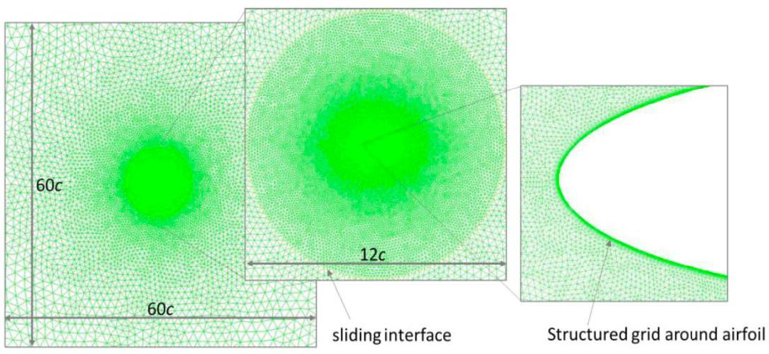
The result is a huge number of unknowns which represent the velocity and pressure at every discrete point in the domain that has been set. If a three-dimensional transient problem is being studied, then there most likely needs to be a huge number of unknowns (velocity and pressure over all space for all time of interest). So grid points in space have time dependent variables at each point and the solution has values at each time for each variable at a location. A small grid space of 1000 elements in each of the three coordinates and for 1000 second duration would represent 1012 data points for each variable of interest. If information at points other than at the given grid are desired they may be interpolated as necessary, but again this will introduce some additional level of error. So the CFD goal is to solve a very large set of algebraic equations written for each discrete position versus time within the flow. As can be imaged the computational efforts can become enormous. Below is an image of a grid developed to study the flow around an airfoil that is oscillating (heaving and pitching) in order to evaluate the aerodynamic forces on the foil with an application of using this motion in a freestream velocity to extract power from the wind.
The Finite Difference Method
An example of applying finite differencing to a simple space dependent problem is shown below, taken from notes generated by Bhaskaran and Collins. Start with the differential equation given by:
[latex]\frac{d u}{d x}+u^{m}=0 ; \quad 0 \leq x \leq 1 ; \quad u(0)=1[/latex]
where “m” is a constant parameter and here we set [latex]m = 1[/latex] (resulting in a linear equation). The selected grid is given below where subscripts on x represent different locations in space with four x locations shown along the x coordinate (the distance between points is constant here and given as [latex]\Delta \text{x}[/latex]:

The equation could be evaluated at each location [latex]x_{i}[/latex] as:
[latex]\left(\frac{d u}{d x}\right)_{i}+u_{i}=0[/latex]
where the subscript [latex]i[/latex] represents the value at grid point [latex]\text{x}_\text{i}[/latex]. An expression for [latex]\left({d u}/{d x}\right)_{i}[/latex] in terms of [latex]u[/latex] at neighboring grid points can be obtained from a Taylor series of [latex]\text{u}_\text{i−1}[/latex]:
[latex]u_{i-1}=u_{i}-\Delta x\left(\frac{d u}{d x}\right)_{i}+O\left(\Delta x^{2}\right)[/latex]
Rearranging gives
[latex]\left(\frac{d u}{d x}\right)_{i}=\frac{u_{i}-u_{i-1}}{\Delta x}[/latex]
Since the Taylor series is truncated after the first derivative there is an error introduced on the first derivative that is of order of the square of the size of the grid, [latex]\left(\Delta \text{x}\right)^2[/latex]. This illustrates the importance of the size of the grid. This error is the “truncation error”. The governing differential equation can be approximated as:
[latex]\frac{u_{i}-u_{i-1}}{\Delta x}+u_{i}=0[/latex]
This resulting algebraic equation for [latex]u_{i}[/latex] simulates the original differential equation but with the truncation error incorporated into it. The error could be reduced by making the grid spacing smaller. Note that an equation of the above form can be written for each grid point in space, resulting in the same number of equations as there are unknown values of the variable, [latex]u_{i}[/latex]. The system of equations would then be solved for all of the unknowns by applying the necessary boundary conditions.
It should be noted that an alternate approach to discretize the governing equations is the Finite volume method. This method provides discrete variable equations, similar to the finite difference method by forming “cells” or small control volumes as seen in the above figure. The conservation equations are written for each cell assuming single valued variables at the faces of each cell. This is a powerful method that has advantages over the finite difference method. But the net result is still a system of equations for the unknown variables for each cell.
System of Equations
As mentioned above we have a system of equations, one for each grid point. However, some of these grids will be at boundaries, in this example they may be at grid points “1” or “4”. Since boundary conditions are needed to be satisfied, they are inserted into the set of equations as known values at these points. Our example is a first order differential equation requiring one boundary condition, which may be at x1. Consequently, there are unknowns of grid points 2, 3 and 4, with a known value at 1. The set of equations now becomes just three equations. In matrix form the equation set becomes:
[latex]\begin{bmatrix} 1 & 0 & 0 & 0 \\ -1 & 1+\Delta x & 0 & 0 \\ 0 & -1 & 1+\Delta x & 0 \\ 0 & 0 & -1 & 1+\Delta x \end{bmatrix} \begin{bmatrix} u_1 \\ u_2 \\ u_3 \\ u_4 \\ \end{bmatrix} = \begin{bmatrix} 1 \\ 0 \\ 0 \\ 0 \end{bmatrix}[/latex]
Note that here the boundary condition equation is included in the matrix. This need not be required by simplifying this to three equations with the boundary condition included in the equation for [latex]\text{u}_\text{2}[/latex]. That is to say the first row and first column in the matrix would be excluded from the matrix above with the value of [latex]\text{u}_\text{1}[/latex] input into the first row of the vector on the right hand side as a known value of “1”.
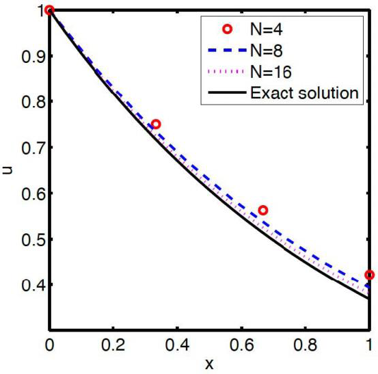
In this simple example it is easy to invert the matrix and calculate the values of [latex]\text{u}_\text{i}[/latex] for a given value of [latex]\Delta \text{x}[/latex]. It is also possible to see that there is an exact solution to this problem, [latex]\text{u = exp(-x)}[/latex]. It is left to the reader to compare results at the discrete points and to show that the difference between exact and approximated values decrease with decreasing values of [latex]\Delta \text{x}[/latex]. It is also seen that as [latex]\Delta \text{x}[/latex] is decreased the number of discrete points increases and the calculation become more complex and time consuming.
This leads to the issue of “grid convergence” – as the grid size is reduced one may expect that the solution would converge to the exact solution. This is illustrated in the figure below, from the notes of Bhaskaren and Collins based on the example above.
Nonlinear Effects
The above example can be expanded in scope by changing the value of the exponent “m” from the value of one. If [latex]\text{m = 2}[/latex] then the second term is nonlinear, [latex]u^2[/latex]. This type of governing equation, with linear and nonlinear terms, is in fact similar to the Navier-Stokes equations where the [latex](\vec{V} \cdot \nabla) \vec{V}[/latex] term is nonlinear.
Going through the same exercise of discretizing the differential term of our example it is shown that the only change to the finite difference algebraic equation is [latex]u^2[/latex]. This could lead to multiple possible solutions. One way to solve this type of system of equations is to “linearize” the equations. This is done by iteration around a guessed value of the variable. That is we assume [latex]u_{i}^{2}[/latex] is [latex]\left(u_{g i}\right) \left(u_{i}\right)[/latex] which is then the product of two different variables, the guessed value [latex]u_{g i}[/latex] and [latex]u_{i}[/latex]. The guessed value is iterated upon until convergence is reached. To do this the difference between the actual and guessed value of [latex]u_{i}[/latex] is denoted as [latex]\Delta u_{i}=\left(u_{i}-u_{g i}\right)[/latex], squaring both sides and solving for [latex]u_{i}^{2}[/latex] results in:
[latex]u_{i}^{2}=u_{g_{i}}^{2}+2 u_{g_{i}} \Delta u_{i}+\left(\Delta u_{i}\right)^{2}[/latex]
Noting that on the right the second term is much larger than the third, since it is expected that [latex]u_{g i}>\Delta u_{i}[/latex], the last term is then neglected. The final expression for [latex]u_{i}^{2}[/latex] is:
[latex]u_{i}^{2} \simeq 2 u_{g_{i}} u_{i}-u_{g_{i}}^{2}[/latex]
where this expression has the inherent error of [latex]O\left(\Delta u_{i}^{2}\right)[/latex]. The right hand side is inserted into the governing equations and the iteration is then applied to the guess values of [latex]u_{g i}[/latex]. An initial guess for [latex]u_{g i}[/latex] is made and solutions are obtained for [latex]u_{i}[/latex], for the now linearized problem. The solution is compared with the guessed values [latex]u_{g i}[/latex], and if different the updated [latex]u_{i}[/latex] is used as the new [latex]u_{g i}[/latex]. This is repeated until the difference between [latex]u_{i}[/latex] and [latex]u_{g i}[/latex] becomes acceptably small. So the solution method is one of solving a linear equation based on an iteration of the linearized term expression.
The “residual” can be defined as the difference between the solution and the guess used at an iteration. An overall residual for the domain can be compiled from residuals at each point as:
[latex]R \equiv \sqrt{\frac{\sum_{i=1}^{N}\left(u_{i}-u_{g_{i}}\right)^{2}}{N}}[/latex]
This provides a measure, on average, of how well all of the grid points are converging. This residual can be scaled with some measure of the value of u throughout the domain, such as the mean value, to provide a measure of residual as a fraction of the mean. Other scaling options are also possible. The “convergence criteria” is measured by the scale residual. In other words a convergence criteria can be set to some small number and the problem is run until that criteria is met. Students can test convergence for this problem, as well as with the exact solution for [latex]m=2[/latex] of [latex]u=1/(1+x)[/latex].
Numerical Stability
The convergence towards a solution is highly dependent on the form of the governing equation and boundary conditions. Convergence may be very fast or slow or never and depends on the numerical solution scheme being used. A “stability analysis” can inform the user what to expect. When a solution does not converge (diverges) the method is “unstable”. A stable method is not necessarily going to results in an accurate solution.
A steady state problem can be solved in different ways. An iterative solution could be used by guessing initial values and trying to converge towards a stable solution. Alternatively, the problem could be solved as a transient problem and started from some initial condition and the transient equations solved over discrete time steps until a steady (non-changing) value is reached. For transient solutions the time step is critical in determining stability. A time step that is too large (which is numerical scheme dependent) can cause the solution to diverge.
Explicit and Implicit Schemes
Whether a method is explicit or implicit is a distinction based on how variables in the equation are solve. Obviously, for a transient problem there is a time dependent term, such as a time derivative. Discretizing this term results in the ratio of the change of variable to the time step interval selected: [latex]\left(u_1^{n+1} - u^n_1\right)/\Delta {t}[/latex], where the superscript on the variable [latex]u[/latex] represents values at time steps n+1 and n, and [latex]\Delta {t}[/latex] is the time interval between time steps. If all other terms in the equation express the variables at time step “n” the only unknown is the variable at the new time step, n+1, since presumably the solution has been found at time step n (or is the initial condition). This is an explicit solution for the variable at time step n+1. These types of equations are stable under a certain constraint on time step and spatial step size conditions. The Courant number is a parameter used to indicate stability and is defined as [latex]C=K \Delta {t}/\Delta {x}[/latex] where the proportionality constant, K, is related to parameters in the problem and has units of distance per time. The value of C is nondimensional and is typically limited to numbers less than one for stability and implies that as the grid size is made larger the allowable time step size can also increase to remain stable. Although large time steps allow for less computational effort, the problem is that as the time step and grid size get large the error also grows.
As an alternative method, the time derivative could be written as a time derivative between time steps n and n-1 (backwards differencing) where the solution is known at n-1 and solved at time step n. Here all other terms in the equation have their variables identified at time step n. In this form the n-1 variables are known and the n variables unknown, and there are multiple unknowns per equation. Each equation can not be solved explicitly but rather a system of equations exist that must be solved implicitly through the entire system of equations for all of the grid points.
In contrast to the above constraint on the time step for explicit solutions through the Courant number, implicit solution schemes tends to be stable for much larger time steps. Note that this does not imply that it is accurate, however, and care must be taken in reaching acceptable levels of numerical errors.
Turbulence Modeling
Fluid flows are often classified as either laminar or turbulent, as discussed in the previous chapters, with a critical Reynolds number often defining where a transition tends to occur. The impact of flows being laminar or turbulent can be enormous. In particular there are consequences relative to wall friction, drag and lift forces, mixing within a fluid, dispersion of species within the flow and heat transfer rates that occur within the fluid and many others. Turbulence is characterized by fluctuations in time and space. The added complexity of turbulent fluid motion occurs over a very wide range of fluctuating time and length scales makes the flow extremely complicated (and interesting!).
The fluctuating variables over time and space give rise to added complexities associated with attempts to solve the Navier-Stokes equations. Using very small time difference, and very small spatial difference to resolve the time and space derivatives allows one to solve the governing equations and basically unravel the turbulent motion. The problem is that these scales become extremely small, particularly for flows with large values of Reynold number. Solutions that use sufficiently small time steps and spatial resolution are called “direct numerical simulations” or DNS and are very computationally expensive. Computing power is no where near sufficient to apply these solutions to reasonably large flows in an economic manner.
An alternative to DNS is to evaluate the time averaged mean quantities only. The need to analyze time averaged turbulent flows has driven the development of highly sophisticated turbulence models so that the need to resolve the very small fluctuations of motion over time and space are not as important. These models must determine the effects of the fluctuating turbulence on the mean flow and incorporate these into the solution for the mean flow variables of velocity and pressure.
The approach to turbulence modeling has evolved over the years as time average representation of the Navier-Stokes equations. As discussed previously, the Reynolds stress, which contains information on the fluctuating velocity, is a consequence of time averaging the nonlinear Navier-Stokes equation, specifically the advection term. This term appears as the time averaged product of fluctuating velocity components (since it is nonlinear). This time average process is called Reynolds averaging where each variable is taken to be the sum of its time averaged mean value and a fluctuating value that varies with time (or [latex]u\left( t \right)=U+u^{\prime}\left( t \right)[/latex] with [latex]U[/latex] being the time averaged value of the velocity and [latex]u^{\prime}[/latex] the fluctuating value about the time averaged value). The mean value is time independent and the fluctuating value varies with time, but has a time average of zero. When each term in the Navier-Stokes equation is time averaged, all fluctuating terms become zero except the nonlinear advection term. Without derivation here we show that the resultant advection term contains the following (where the overbar is the time average):
[latex]\frac{\partial\left(\rho \overline{u_{i}^{\prime} u_{j}^{\prime}}\right)}{\partial x_{j}}[/latex]
The following model is used:
[latex]\rho \overline{u_{i}^{\prime} u_{j}^{\prime}}=2 \mu_{t} S_{i j}-\frac{2}{3} \rho k \delta_{i j}[/latex]
[latex]S_{i j}=\frac{1}{2}\left(\frac{\partial U_{i}}{\partial x_{j}}+\frac{\partial U_{j}}{\partial x_{i}}\right); \quad k=\frac{1}{2} \overline{u_{i}^{\prime} u_{i}^{\prime}}[/latex]
The terms in this model are explained as follows. The advection term is the spatial derivative of [latex]\left(\rho \overline{u_{i}^{\prime} u_{j}^{\prime}}\right)[/latex], which has units of [latex]N/m^2[/latex] per volume of fluid in SI units, equivalent to a stress per volume, the so called Reynolds stress or turbulent stress. Since this term appears as a spatial derivative of a stress, a possible model would be to mimic the laminar stress model and express the “turbulent stress” as the product of a “turbulent viscosity”, [latex]\mu_t[/latex], times the strain rate tensor, [latex]S_{i j}[/latex], shown above. The model also includes the parameter [latex]k[/latex], known as the turbulent kinetic energy. In using this model the turbulent stress is replaced by an unknown turbulent viscosity [latex]\mu_t[/latex] and [latex]k[/latex]. The turbulent viscosity is dependent on the turbulence in the flow, rather than just the fluid as in the laminar case. A model needs to be developed to determine both the turbulent viscosity and turbulent kinetic energy. A model for these turbulent parameters is not easy and there are several that have been proposed.
If the turbulent viscosity is to model the added mixing of momentum caused by the turbulent flow, then one approach is to relate this to the turbulent energy of the turbulence, [latex]k[/latex]. This energy, which is the energy per mass of fluid, is defined as one half of the time average of the square of the fluctuating velocity. The greater the amplitude of the fluctuating velocity the greater the turbulent kinetic energy.
Also, the turbulent viscosity is assumed to be dependent on how much the turbulent kinetic energy is dissipated by the friction occurring with the surrounding fluid. The “turbulent dissipation”, [latex]\varepsilon[/latex], is defined as the rate of loss of [latex]tke[/latex] and has units of energy per time per mass of fluid, or [latex]m^2/s^3[/latex].
If the assumption is made that [latex]\mu_t=\rho \nu_t[/latex] (where [latex]\nu_t[/latex] is the turbulent kinematic viscosity) and that [latex]\nu_t=f(k,\varepsilon)[/latex] then by dimensional analysis (where the units of the turbulent kinematic viscosity, [latex]\nu_t[/latex] are [latex]m^2/s[/latex]) a form of this function could be: [latex]\nu_t=C_\mu \left(k^2/\varepsilon\right)[/latex], where [latex]C_\mu[/latex] is an empirical nondimensional constant of 0.09. Taking this approach the problem as reverted to knowing the local distribution of [latex]k[/latex] and [latex]\varepsilon[/latex] and from this being able to calculate [latex]\nu_t[/latex] at each point in the flow and then use this to calculate the Reynolds stress from the above model. This stress can be inserted into the Navier-Stokes equations and solved for the time averaged mean velocity and pressure.
To complete the model two additional transport equations, one each for [latex]k[/latex] and [latex]\varepsilon[/latex], are derived from the time varying Navier-Stokes equations. The result is two differential equations that need to be solved at each grid location (or cell if using a finite volume method). This is known as the two equation turbulence model. This results in significant computation effort added to the solution of the mean Navier-Stokes equations (one for each coordinate direction).
There are a number of similar turbulence models that are available in most commercial software packages. The “best” one to use depends on the flow conditions and the accuracy is typically dependent on the computational expense. It is very important to be aware of limitations of the various models which is usually described for the software user in these commercial software packages. The result is a solution for the mean, time averaged, variables.
