VII. Introduction to Viscous Flows
In this section we develop the governing equations for viscous flows resulting in the Navier-Stokes equations. We will simplify the equations for incompressible constant property flows, which are useful for a vast majority of flow situations. We will then show how this seemingly formidable set of equations can be simplified for a number of rather practical flow problems resulting in exact, analytical solutions. We end with the introduction to similarity solutions to the Navier-Stokes equations through an example problem.
Basics of Viscous Forces
The introduction of viscous forces requires a model to obtain a set of conditions on the flow field to express the viscous stress tensor, [latex]{\tau }_{ij}[/latex], as a function of the local velocity field. This stress tensor consists of the various stresses that can occur on an element of fluid. These forces act at the surface of a fluid element and are caused by a velocity gradient normal to the surface. This velocity gradient can give rise to local friction. In regions of the flow where the velocity gradients go to zero we expect there to be no viscous forces acting. We will show that even though viscous forces may not be zero due to existing velocity gradients their net effect may in fact be zero on a fluid element when taking into account all viscous forces over all the surfaces of an element. Additionally, it is possible to have velocity gradients and no net viscous forces. This will be evident once we present a model equation describing the viscous forces.
By including viscous forces in the flow we need to introduce the no-slip boundary condition, whereby the fluid in contact with a surface takes on the same velocity as the surface — the fluid is not allowed to “slip” along the surface. In doing this a velocity profile is set up across the flow direction. For example in pipe flow the fluid velocity at the pipe wall is the same as the velocity of the pipe, but to have a net flow through the pipe fluid away from the wall is moving differently than the pipe. If the pipe is circular the center of the pipe is furthest from the walls and the fluid in this portion of the pipe is traveling fastest. So for a circular pipe the flow is symmetric circumferentially with a maximum in the center. For pipes with different cross sections we still expect a peak velocity in the region furthest from all walls, since the impact of the wall friction is furthest away. Friction occurs throughout the cross section however, not just at the walls. This internal friction is fluid-fluid friction due to the fact that different “layers” of fluid, or fluid elements are moving at different velocities.
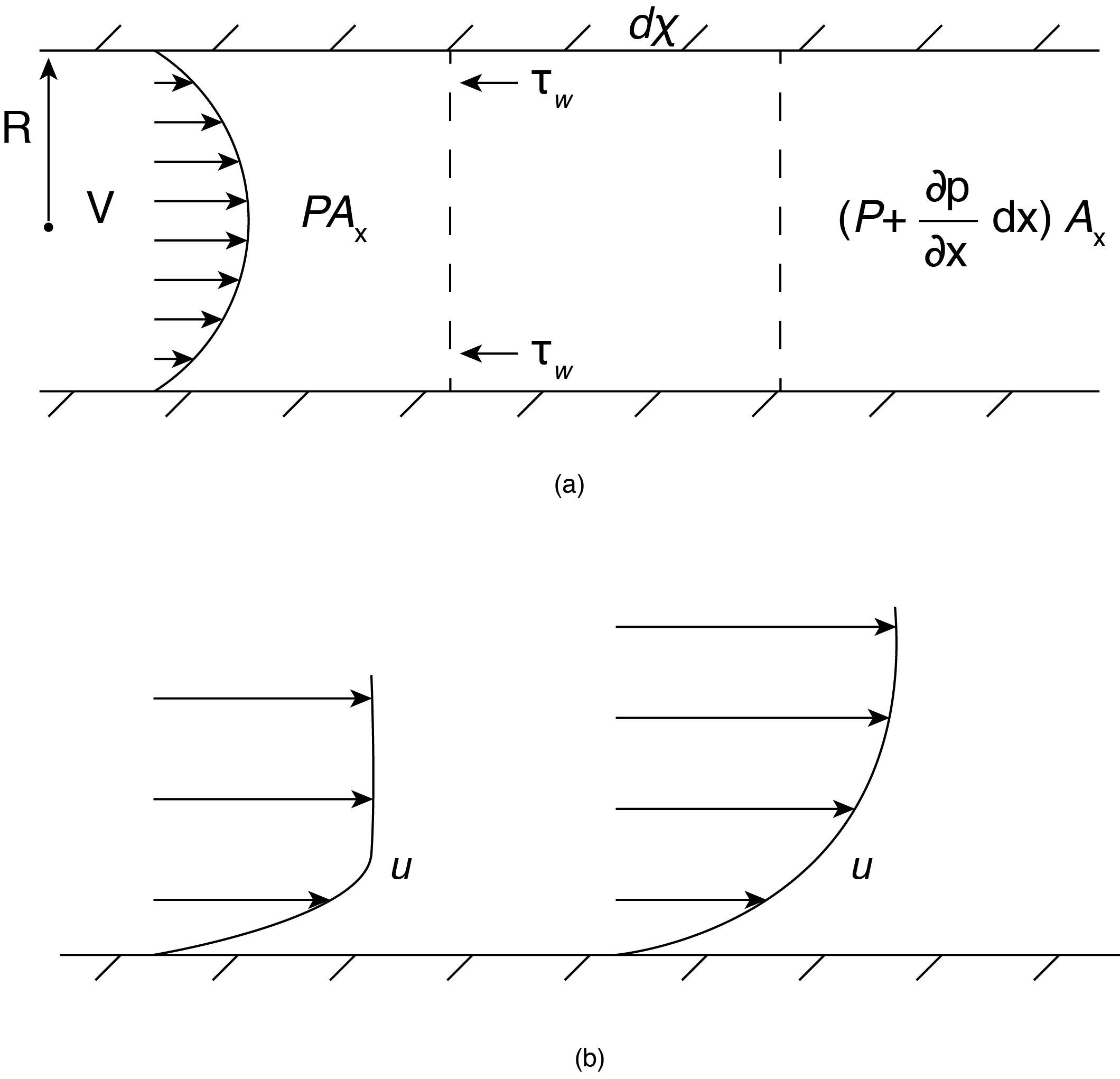
For laminar pipe flows, which most readers have seen in their first course in fluid mechanics, there are some characteristic conditions we can discuss that are relevant to internal viscous flows in general. In the case of steady, fully developed flow we can set a force balance to better understand the required forces acting on the fluid. We will define this characterization of the flow (steady, fully developed) in a later part of this chapter, in reference to the governing equation. Referring to Fig. 7.1 (a) for the illustrated control volume of length dx extending across the area of the round pipe of radius R we see that a force balance for nonaccelerating flow between the force due to pressure and that due to wall friction becomes:
[latex]\frac{dP}{dx}=-\frac{2\pi R}{\pi R^2}{\tau }_w=-\frac{2{\tau }_w}{R}\tag{7.1}[/latex]
This indicates that the pressure decreases along the flow direction proportional to the magnitude of the wall shear stress caused by friction between the fluid and pipe wall. In this equation the values of the wall shear stress is taken as a positive number.
External flows have a similar no-slip condition at a surface, the difference being that as one moves away from the surface any other boundaries are “infinitely” far away in the sense that these other surfaces are not influencing the flow. This is shown in Fig. 7.1 (b) showing that the extent of the friction layer increases along the flow direction. However, there is still wall friction and fluid-fluid friction up to some point far enough from the surface, which depends on the particular location along the surface. We will discuss this in detail when we examine boundary layer flows. Recall that in previous sections we neglected viscous effects for external flows and the results tend to be very accurate, this is because for the flows we looked at other forces that come into play (pressure and body forces) dominate the flow. However, even in these flows viscous forces can be important in that they lead to “flow separation” where streamlines no longer follow the general shape of the object. When this occurs the potential flow solutions tend to break down, even though pressure forces dominate the overall forces. This is because the velocity distribution is greatly altered by the flow separation. This topic of flow separation is beyond the scope of this book but we will discuss it to a limited extent in the next chapter. The reader is referred to “Viscous Fluid Flow” by F.M. White for a discussion of this and some of the many models used in these flows, to predict wall friction effects.
The velocity profiles shown in Fig. 7.1 indicates a variation of velocity from the boundary condition at the surface of no-slip to a maximum at the centerline for pipe flow or reaching the freestream velocity far from the surface in external flows. This implies a distribution of internal viscous stress caused by the local velocity distribution since frictional forces depend on the relative velocity variation, or velocity derivative, within the flow field. In order to determine the magnitude of these forces we will first define the viscous stress tensor.
Viscous Stress
Viscous forces are represented here using the viscous stress tensor, [latex]{\tau }_{ij}[/latex], that contains nine possible elements in three-dimensional space, three diagonal elements, i=j, and six off diagonal terms. Each of these terms will be given an interpretation relative to the flow. Physically the viscous stress is linked to the velocity gradient that results in a strain rate acting on a fluid element. Recall that fluids can have a continuous deformation with an applied force, in contrast to a solid which may have a given deformation proportional to the applied stress. We anticipate a relationship between the stress and the resultant strain rate occurring in the fluid. So first we define the strain rate that occurs within the fluid.
A small fluid element is shown in Fig. 7.2. First consider Fig. 7.2 (a) showing a “linear strain”. Assume there exists an increase of [latex]{u}_{1}[/latex] in the [latex]{x}_{1}[/latex] direction, [latex]\frac{\partial u_1}{\partial x_1}dx_1[/latex], as a result, the surface of the element on the right (at larger [latex]{x}_{1})[/latex] will move faster to the right than the surface on the left (at smaller [latex]x_{1}[/latex]). Over time [latex]\Delta t[/latex] the distance between the two surfaces, denoted as “l” which is originally [latex]dx{}_{1}[/latex] will increase by [latex]\Delta l[/latex] leading to a rate change of separation distance, or a rate of deformation equal to:
[latex]\frac{1}{l}\left ( \frac{\bigtriangleup{l}}{\bigtriangleup{t}} \right )=\frac{\bigtriangleup{l/l}}{\bigtriangleup t}=\frac{\partial u_1}{\partial x_1}\tag{7.2}[/latex]
Treating [latex]\Delta l/l[/latex] as the strain then Eqn. (7.2) represents the linear strain rate in the [latex]x{}_{1}[/latex] direction caused by the [latex]u{}_{1}[/latex] velocity gradient in the [latex]x{}_{1}[/latex] direction. We can write similar expressions for the [latex]x{}_{2}[/latex] and [latex]x{}_{3}[/latex] directions as [latex]\frac{\partial u_2}{\partial x_2}[/latex] and [latex]\frac{\partial u_3}{\partial x_3}[/latex], respectively. Physically, for positive values of these velocity gradient components in each direction we see that there is a stretching in each direction, there is similar compression if the derivatives are negative. There is a change of volume per time of [latex]\frac{\left ( \bigtriangleup l/l \right )_1}{\bigtriangleup t}\left ( \partial x_1 \partial x_2 \partial x_3 \right )=\frac{\partial u_1}{\partial x_1}\left (\partial x_1 \partial x_2 \partial x_3 \right )[/latex]. Similarly in all 3 directions. Taken together over time there is a change in volume of the fluid element measured by the sum of the total change in each direction. Dividing through by volume [latex]\left (\partial x_1 \partial x_2 \partial x_3 \right )[/latex] we call this result the “dilation rate” of the fluid. Using tensor notation we can write the dilation rate (using the summation rule) as:
[latex]\frac{\partial u_i}{\partial x_i}={\dot{e}}_{ii}\tag{7.3}[/latex]
(Where summation is implied)
The units of [latex]{\dot{e}}_{ii}[/latex] are one over time.
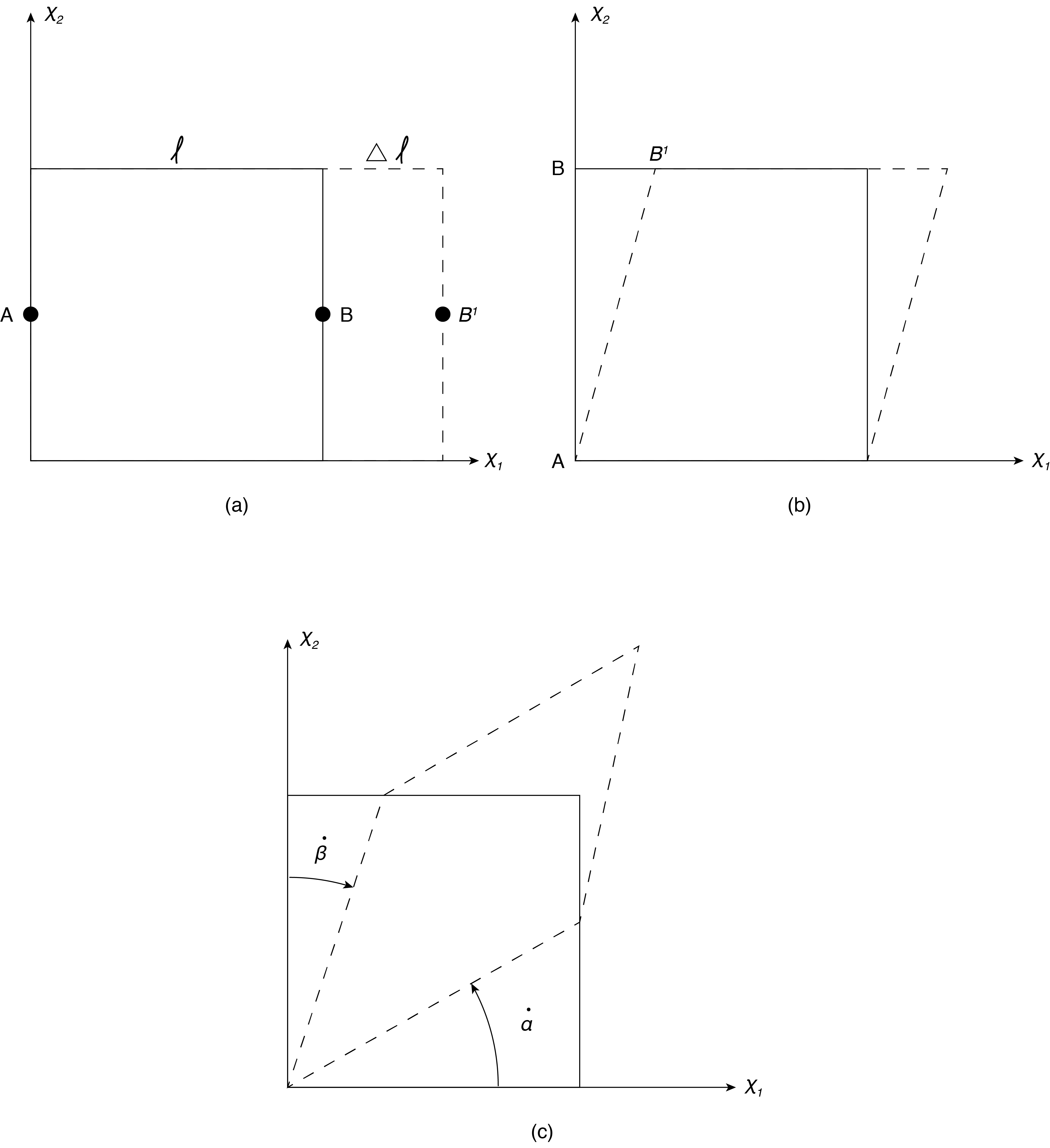
Now consider Fig. 7.2 (b), which shows the shear strain rate. Or the rate of strain caused by a shearing force. In this case two points on the element surface, A and B, will have a change of orientation relative to a fixed coordinate system. So points A-B will move to A-B’ if the [latex]x{}_{1}[/latex] component of velocity increases in the [latex]x{}_{2}[/latex] direction. As shown this can be interpreted as a rotation of the line connecting A-B. If distance B-B’ is length [latex]\Delta l[/latex] and the line length A-B = [latex]dx_2=l[/latex] then:
[latex]\frac{\Delta l/l}{\Delta t}=\frac{\partial u_1}{\partial x_2}\tag{7.4}[/latex]
We can interpret this as a rotation, or angular strain rate, which in this case is about the [latex]x{}_{3}[/latex] axis. Similarly there can be a rotation about [latex]x_3[/latex] caused by rate, [latex]\frac{\partial u_2}{\partial x_1}[/latex]. This can be repeated to obtain angular strain rates about each of the other axes as well.
These results provide the basis for the definition of the strain rate tensor, [latex]{\dot{e}}_{ij}[/latex]:
[latex]{\dot{e}}_{ij}=\frac{1}{2}\left(\frac{\partial u_i}{\partial x_j}+\frac{\partial u_j}{\partial x_i}\right)\tag{7.5}[/latex]
Notice that when i=j the strain rate tensor consists of components of the dilation rate, for instance [latex]\frac{\partial u_1}{\partial x_1}[/latex], etc. When [latex]i\neq j[/latex] we see the addition of the two terms causing rotation about any given axis. For instance if i=1 and j=2 we obtain rotation about the [latex]x{}_{3}[/latex] axis as shown above. But also, if i=2 and j=1 we also obtain rotation about the [latex]x{}_{3}[/latex] axis. In fact when added to calculate [latex]{\dot{e}}_{ij}[/latex] these resultant two cases are identical in value. This implies that the strain rate tensor is symmetric, [latex]{\dot{e}}_{ij}={\dot{e}}_{ji}[/latex]. Keep in mind that when the velocity derivative component is negative we have rotation in the opposite direction. The sign convention is that counter-clockwise rotation is positive. The inclusion of ½ is a matter of convenience as we will see later, but also can be thought of as providing an average of the two terms.
The general strain rate tensor, [latex]{\dot{e}}_{ij}[/latex], consists of all possible combinations of velocity spatial derivatives, and contains 9 elements. The diagonal terms are “linear deformation rates” and the off diagonal terms are the “shearing deformation rates”. Notice that there are really only six definitive terms, since this is a symmetric tensor.
Recall that vorticity, is a measure of rotation rate as well. We need to distinguish this from the strain rate tensor. Consider the case of [latex]\ {\omega }_3[/latex]:
[latex]{\omega }_3=\left(\frac{\partial u_2}{\partial x_1}-\frac{\partial u_1}{\partial x_2}\right)\tag{7.6}[/latex]
First we notice the sign difference for the second term in the parenthesis when compared with the strain rate tensor. What is the consequence of this? If rotation caused by [latex]\frac{\partial u_2}{\partial x_1}[/latex] is counter clockwise because this derivative is positive, and the rotation caused by [latex]\frac{\partial u_1}{\partial x_2}[/latex] is negative when this derivative value is positive, then applying this to the above definition of [latex]{\omega }_3[/latex] results in a net positive rotation (counter clockwise) about the [latex]x{}_{3}[/latex] axis. Or said another way, the vorticity is the sum of the two contributions of positive rotation rate about a given axis. Notice that vorticity has only three terms needed to define it (hence it is a vector). The diagonal terms are identically zero and the off diagonal terms are just of opposite sign (an antisymmetric tensor).
It is then possible to have zero vorticity (the two terms in the vorticity definition cancel) but still have a positive angular deformation. Consider the case of [latex]\frac{\partial u_2}{\partial x_1}=\frac{\partial u_1}{\partial x_2}[/latex] where the rotation rate is zero but the net angular deformation rate is not, and equal to twice the value of each component. This addition is shown schematically for a fluid element in Fig. 7.2 (c) where the net rotation about the [latex]x{}_{3}[/latex] axis would be zero if [latex]\dot{\alpha }=\ \dot{\beta }[/latex] , but we see deformation of the fluid element.
We do one last manipulation. Suppose we identify the velocity gradient tensor as [latex]\frac{\partial u_i}{\partial x_j}[/latex]. This has nine elements of all of the partial derivatives of the three components in the three coordinate directions. This second order tensor can be written as:
[latex]\frac{\partial u_i}{\partial x_j}=\frac{1}{2}\left(\frac{\partial u_i}{\partial x_j}+\frac{\partial u_j}{\partial x_i}\right)+\frac{1}{2}\left(\frac{\partial u_i}{\partial x_j}-\frac{\partial u_j}{\partial x_i}\right)\tag{7.7}[/latex]
The first term on the right hand side is the deformation rate tensor and the second term is ½ of the vorticity, which (when including the ½) is identified as the rotation rate tensor. The latter can be thought of as the average rotation about any given axis. So the velocity gradient tensor consists of two parts, that due to the strain rate and that due to the vorticity (or rotation rate).
At this point we will construct a fairly simple model for the relationship between viscous stress and deformation rate to be as follows:
[latex]{\tau }_{ij}\sim {\dot{e}}_{ij}[/latex]
This implies that the rate of deformation that occurs in a fluid element is directly proportional to the stress applied to that element. If we make the assumption that there is a proportionality factor equal to 2 [latex]\mu[/latex], then we can write this as:
[latex]{\tau }_{ij}=\mu \left(\frac{\partial u_i}{\partial x_j}+\frac{\partial u_j}{\partial x_i}\right)\tag{7.8}[/latex]
It is obvious why the factor 2 was introduced. Notice that the relationship does not include any of the rotational components of the velocity gradient tensor, only the deformation rate components. The physical interpretation is that viscous stress is related to the degree of deformation occurring in a fluid element, not its rotation rate.
Looking at the normal stress components, when [latex]{i=j}[/latex], we see that these terms result in linear deformation. As noted above these are elongation or contraction rates of a fluid element as it flows over time. Adding all three dimensions we get the net volume change of the fluid element over time. Consequently, according to the model of Eqn. (7.8) the viscous forces resulting in normal viscous stress components are responsible for these linear deformation rates. These stresses are the normal, or diagonal, components of [latex]{\tau }_{ij}[/latex].
The shearing contributions of [latex]{\tau }_{ij}[/latex] are the off diagonal terms and are related through Eqn. (7.8) to the off diagonal terms of the strain rate tensor, [latex]{\dot{e}}_{ij}[/latex]. These terms result in an angular deformation rate that distorts the original shape of the fluid element over time. Again, according to eqn. (7.8) this angular deformation rate, due to shearing viscous stresses, has a magnitude determined by the parameter, [latex]\mu[/latex].
The parameter [latex]\mu[/latex] is a fluid property and can take on many forms depending on the characteristics of the fluid itself. This property is the fluid dynamic viscosity and may be a function of the state of the fluid (say its pressure or temperature), but it may also be a function of the stresses applied to the fluid. A Newtonian fluid is one that can have state varying viscosity (say like an oil that has decreasing viscosity with increasing temperature) but has a constant value of viscosity with changing stress within the fluid. These fluids have a linear relationship between viscous stress and deformation rate.
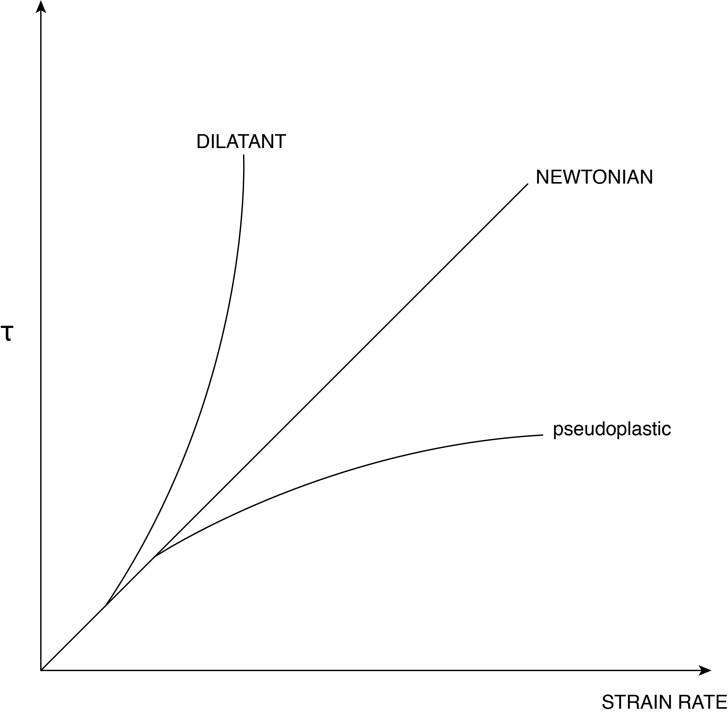
A dilatant fluid is described as shear thickening. That is to say as a shearing stress is applied to the fluid the viscosity increases. This implies that increasing stresses will result in decreasing deformation rates, consequently not having a linear relationship. Mixtures of cornstarch and water can behave as a dilatant fluid. In contrast, a fluid with a decreasing viscosity with increasing applied stress is called pseudo-plastic, or shear thinning, fluids. Examples of this type of behavior is ketchup, some paints, ink, and others. Fig. 7.3 illustrates the stress-strain rate relationship for various types of fluids where the slope is a measure of viscosity. For the remainder of this book we will deal with Newtonian fluids. Keep in mind, however, functional relationships can be used for non-Newtonian fluid viscosities, whereas we will use constant values in the problems we examine.
Navier-Stokes Equation
The Navier-Stokes equation is an extension of Euler’s equation with the addition of the viscous forces. The Euler equation is written as:
[latex]\rho \frac{Du_i}{Dt}=\frac{\partial P}{\partial x_I}+\rho g_i[/latex]
which is a balance of mass times acceleration per volume on the left hand side with the net force due to pressure gradients and the gravitational body force, both per volume of fluid. It should be noted that if we combine the pressure terms with the viscous stress terms we obtain the combined total stress expression:
[latex]{\sigma }_{ij}=-P{\delta }_{ij}+{\tau }_{ij}\tag{7.9}[/latex]
We use the Kronecker delta, [latex]{\delta }_{ij}[/latex], which is equal to one when i=j and otherwise equal to zero. This conveniently indicates that P is a normal compressive stress component. The negative sign indicates that pressure is compressive.
An additional force is introduced to account for forces that result in volume changes of a given fluid element. This is modeled as follows. As noted above the rate change of fluid volume per original volume is given by [latex]\frac{\partial u_k}{\partial x_k}[/latex], where there is summation over index k. Assuming that the force required to change the volume is a compressive normal force, and proportional to the volume change, we can write this force as:
[latex]\lambda \frac{\partial u_k}{\partial x_k}{\delta }_{ij}[/latex]
where [latex]\lambda[/latex] is a proportionality constant dependent on the fluid. This is added to the above stress expression to yield:
[latex]{\sigma }_{ij}=-P{\delta }_{ij}+{\tau }_{ij}+\lambda \frac{\partial u_k}{\partial x_k}{\delta }_{ij}\tag{7.10}[/latex]
The net force per volume of fluid due to the stress can be written as:
[latex]\frac{\partial {\sigma }_{ij}}{\partial x_j}\tag{7.11}[/latex]
Recall that there is a summation over the index j indicating that this expression is in a vector in the i direction. Inserting Eqn. (7.8) for the stress term in Eqn. (7.10), and then insert this result into Eqn. (7.11) results in the net stress force on a fluid element. This is then added to the Euler equation keeping in mind that we have already included the pressure term with the stresses. The result is:
[latex]\rho \frac{Du_i}{Dt}=\frac{\partial {\sigma }_{ij}}{\partial x_j}+\rho g_i=-\frac{\partial P}{\partial x_j}{\delta }_{ij}+\frac{\partial }{\partial x_j}\left(\lambda \frac{\partial u_k}{\partial x_k}\right){\delta }_{ij}+\rho g_i+\frac{\partial }{\partial x_j}\ \left(\mu \left(\frac{\partial u_i}{\partial x_j}+\frac{\partial u_j}{\partial x_i}\right)\right)\tag{7.12}[/latex]
This equation has three velocity components and the pressure as unknowns. Two fluid parameters, [latex]\mu[/latex] and [latex]\lambda[/latex] are also included. The parameter [latex]\lambda[/latex] is known as the coefficient of bulk viscosity, and is representative of the force required to change the fluid volume.
For an incompressible fluid, since [latex]\frac{\partial u_k}{\partial x_k}=0,[/latex] (with summation) this term disappears.
For a compressible fluid Stokes hypothesis is that:
[latex]\lambda =-\frac{2}{3}\mu\tag{7.13}[/latex]
This comes with some theoretical justification and has been shown over a wide range of conditions to be reasonably valid, but shown not to be valid for extreme pressures. Since in this book we restrict ourselves to incompressible flows, this is not an issue and we will neglect this term. Also, for incompressible flows with constant viscosity we can simplify the last (viscous) term in Eqn. (7.12) as:
[latex]\frac{\partial }{\partial x_j}\ \left(\mu \left(\frac{\partial u_i}{\partial x_j}+\frac{\partial u_j}{\partial x_i}\right)\right)=\mu \frac{{\partial }^2u_i}{\partial {x_j}^2}+\mu \left(\frac{\partial }{\partial x_i}\left(\mu \frac{{\partial }u_j}{\partial {x_j}}\right)\right)=\mu \frac{{\partial }^2u_i}{\partial {x_j}^2}\tag{7.14}[/latex]
wherein the second term in the middle expression we have reversed the order of differentiation of [latex]x{}_{i}[/latex] and [latex]x{}_{j}[/latex] and then invoked the incompressible condition leaving only the first term, which is the Laplace of the velocity vector.
The final form of the Navier-Stokes equation that we will use for incompressible constant viscosity (Newtonian fluid) flows is:
[latex]\rho \frac{Du_i}{Dt}=\rho \frac{\partial u_i}{\partial t}+\rho u_j\frac{\partial u_i}{\partial x_j}=-\frac{\partial P}{\partial x_j}{\delta }_{ij}+\rho g_i+\mu \frac{{\partial }^2u_i}{\partial {x_j}^2}\tag{7.15}[/latex]
The left hand side has been expanded to show the local and convective acceleration terms and on the right hand side we have force contributions from pressure gradients, gravity and viscous forces (normal and shearing). This equation is coupled with the requirements for incompressible flow:
[latex]\frac{\partial u_k}{\partial x_k}=0\tag{7.16}[/latex]
Notice, since we have incompressible flow it is possible to rewrite the convective acceleration term:
[latex]\rho u_j\frac{\partial u_i}{\partial x_j}=\rho \frac{\partial \left(u_iu_j\right)}{\partial x_j} \tag{7.17}[/latex]
Sometimes this may be referred to as the “conservative form” of the Navier-Stokes equation since it takes advantage of the conservation of mass for incompressible flow.
We can also rewrite the Navier-Stokes equation using the definition of vorticity. First the convective acceleration term invokes the vector identity mentioned, in an earlier chapter in discussion of the generalized Bernoulli equation, that is written as:
[latex]\rho u_j\frac{\partial u_i}{\partial x_j}=\ \rho \left(\frac{\partial \left(\frac{1}{2}u_ju_j\right)}{\partial x_i}+{\varepsilon }_{ijk}{\omega }_ju_k\right)\tag{7.18}[/latex]
The viscous terms can also use the following vector identity:
[latex]\mu \frac{{\partial }^2u_i}{\partial {x_j}^2}=-\mu {\varepsilon }_{ijk}\frac{\partial {\omega }_k}{\partial x_j} \tag{7.19}[/latex]
This last term is the viscosity times the curl of the vorticity. Notice what happens when the flow is irrotational. The second term of Eqn. (7.18) is zero and the viscous stress term, Eqn. (7.19), is also zero. It is left for the reader to see that under these conditions one can arrive at the simplified Bernoulli equation when integrated between any two points within the flow field. If the flow is inviscid the last term of Eqn. (7.15) is zero, but the flow is not necessarily irrotational since the vorticity also enters into the equation in the convective acceleration term. So, an irrotational flow does imply an inviscid flow but an inviscid flow does not imply irrotational flow. Lastly, the viscous term vanishes if the curl of the vorticity is zero, it is not necessary that the flow be irrotational.
Examples of Exact Solutions to Navier-Stokes Equation
Steady Flow Between Parallel Plates or in a Circular Pipe
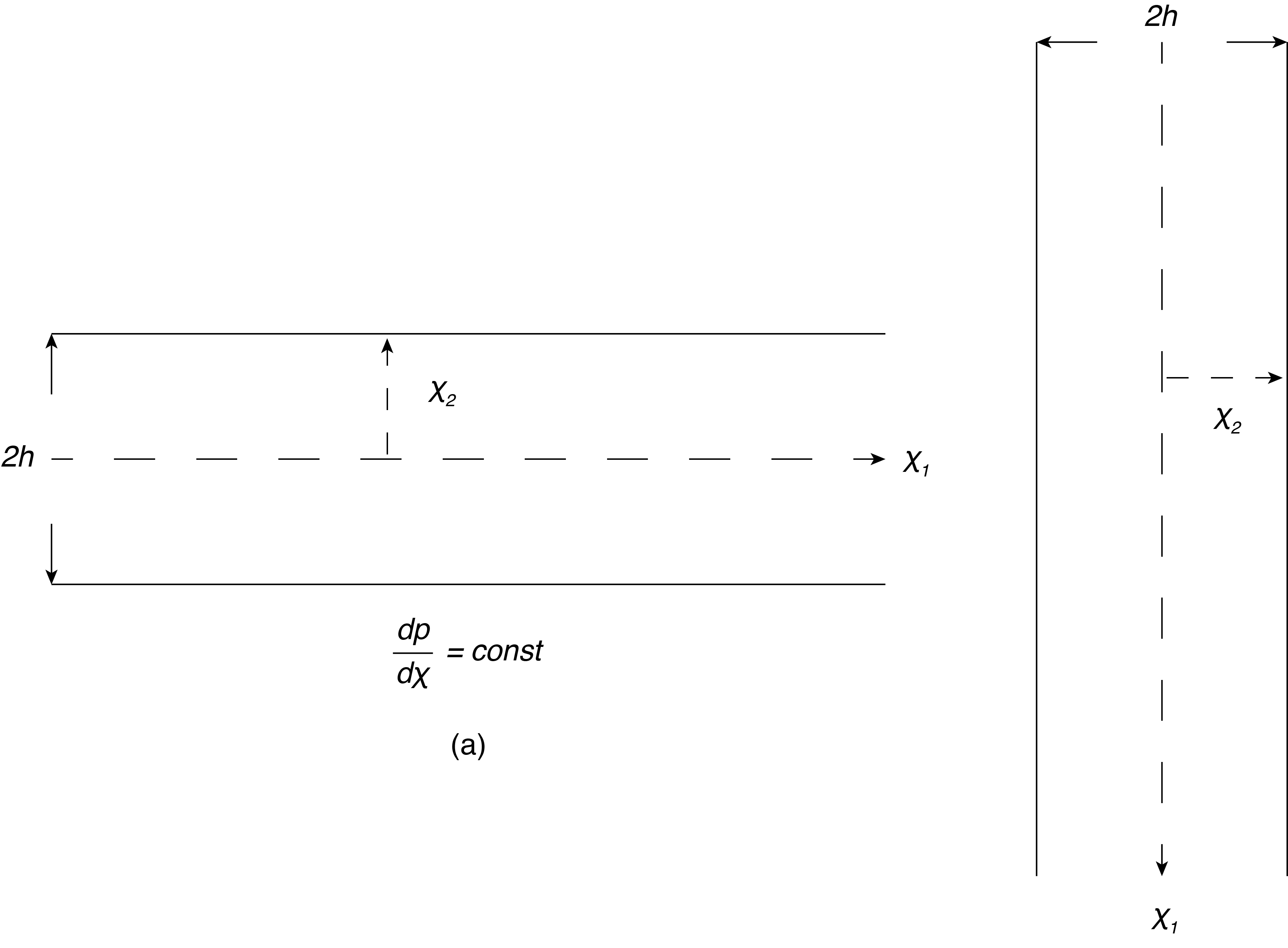
For fully developed, steady flow between parallel plates shown in Fig. 7.4 using Cartesian coordinates with flow in the [latex]x{}_{1}[/latex] direction the reader should verify that there is no acceleration and the Navier-Stokes equation reduces to a balance of forces. If the flow is horizontal there is only pressure and viscous forces that balance. If the flow is vertical with no pressure driving the flow then there is a balance of gravitational forces and viscous forces. For plates with a separation distance of 2h with the [latex]x{}_{1}[/latex] axis along the centerline between the plates, as shown in the figure, the form of the velocity distribution in both cases is identical. Note that since there is only the [latex]{u_1}[/latex] velocity component then [latex]\frac{\partial u_1}{\partial x_1}=0[/latex] and we say the flow is fully developed, with no changes in the flow direction and no convective acceleration. For steady flow there is no local acceleration.
Consider horizontal flow, so no body force, to determine the velocity distribution we first examine the pressure gradient term for this case. Since there is no acceleration the pressure term is balanced by the viscous terms. The resulting Navier-Stokes equation is:
[latex]0=-\frac{\partial P}{\partial x_j}{\delta }_{ij}+\mu \frac{{\partial }^2u_i}{\partial {x_j}^2}=\frac{dP}{dx_1}+\mu \frac{d^2u_1}{dx_2 ^2}[/latex]
To explain why we can write the terms as ordinary derivatives consider the following. Since the acceleration is zero we can say that [latex]u_1\neq f(x_1)[/latex] which is also found from the conservation of mass noting that [latex]u{}_{2}=u{}_{3}=0[/latex]. Based on this we can say that the viscous term is not a function of [latex]x{}_{1}[/latex], so therefor the pressure term is not a function of [latex]x{}_{1}[/latex] either. At most [latex]u{}_{1}[/latex] is a function of [latex]x{}_{2}[/latex]. One can show that [latex]dP/dx{}_{1}[/latex] is not a function of [latex]x{}_{2}[/latex] from the [latex]x{}_{2}[/latex] momentum equation. So if the change of P along the flow is not a function of [latex]x{}_{2}[/latex] or [latex]x{}_{1}[/latex], then [latex]dP/dx{}_{1}[/latex] is a constant.
By applying the no-slip boundary condition at the wall surfaces, [latex]x{}_{2}[/latex] = +/- h the result is:
[latex]u_1=C\left(1-\frac{{x_2}^2}{h^2}\right)\tag{7.20}[/latex]
where [latex]C=-\frac{h^2}{2\mu }\frac{dP}{dx_1}[/latex] for pressure driven horizontal flow and [latex]C=\frac{\rho gh^2}{2\mu }[/latex] for gravity driven vertical downward flow.
Given this velocity field the vorticity distribution can be determined and since the velocity is parabolic the vorticity distribution will be piecewise linear across the flow with zero value at the center, and maximum value at the surface, [latex]{\omega }_3=-\frac{2C}{h^2}x_2[/latex].
The same flow can be considered for flow in a round constant area horizontal pipe. This is often called Hagen-Poiseuille flow after two experimentalists who developed this relationship in the 1800s for steady pipe flow in the form of flow rate versus pressure drop. In this case the Navier-Stokes equation is written in cylindrical coordinates as shown in Table 7.1 and then reduced for steady, constant area, incompressible, constant property flow. Again, the flow has no acceleration for steady, constant area flow and the result is a balance of pressure and viscous forces in the [latex]z[/latex], or axial direction. The pressure gradient along z is a constant similar to the result for flow between parallel plates. The resulting simplified equation is integrated across the flow (r coordinate) using the no-slip boundary condition at [latex]r=R[/latex] ([latex]R[/latex] is the pipe radius) and also noting that the velocity is a maximum at the centerline where the velocity derivative in [latex]r[/latex] is zero. The result is:
[latex]v_z=-\frac{R^2}{4\mu }\frac{dP}{dz}\left(1-\frac{r^2}{R^2}\right)\tag{7.21}[/latex]
For all of these internal flows the flow rate can be obtained by integrating the velocity distribution across the flow area. For instance, for a volumetric flow rate of [latex]\dot{Q}[/latex] and writing the pressure gradient [latex](-dP/dx_1)[/latex] as [latex]\Delta P/L[/latex] since it is constant (notice the sign change since [latex]\Delta P[/latex] is the upstream pressure minus the downstream pressure) and [latex]L[/latex] is the total length along [latex]x{}_{1}[/latex]. We have for steady horizontal pressure driven flow between parallel plates:
[latex]\dot{Q}=\frac{2h^3\Delta P}{3\mu L} l \text{ (per distance }x_3\text{)}\tag{7.22}[/latex]
For steady flow in a pipe:
[latex]\dot{Q}=\frac{\pi R^4\Delta P}{8\mu L}\tag{7.23}[/latex]
It is straight forward to evaluate similar relationships for gravity driven flows by replacing the pressure gradient with [latex]\rho g[/latex].
There are a number of other steady flows that can also be solved for analytically from the Navier-Stokes equation. For instance, steady axial flow in an annulus, either pressure or gravity driven; flow in the gap between two rotating cylinders that have different rotation rates; flow between parallel plates where one plate is moving relative to the other with or without a pressure gradient or gravity driving the flow, and a few others. All of these flows have no local or convective acceleration terms and the basic governing equation is a balance of forces. It is possible to solve some flows with acceleration as shown next.
Suddenly Accelerated Plate (Stokes First Problem, also known as the Rayleigh Problem)
When a flat plate is immersed in a large body of fluid, and the plate is suddenly accelerated to some fixed, constant velocity the fluid surrounding the plate will be set into motion. This general problem is known as Stokes first problems, named for Sir George Stokes the well-known mathematician, for whom the Navier-Stokes equation is also named. There are variations on this problem, such as the flow field set up in a fluid when the plate oscillates back and forth sinusoidally, Stokes second problem. Here we will look at the solution one can obtain for the first problem. It will introduce the idea of a similarity formulation of the problem and provide insight on how to nondimensionalize results. It is also useful in the interpretation of boundary layer flows that we will examine in a later chapter.
This is an idealized problem where the plate is assumed to accelerate instantaneously to some velocity [latex]U=U{}_{p}[/latex] and remains at that velocity. Obviously there is some finite time for this to happen, but we ignore that (short) time effect. Fig. 7.5 illustrates the coordinate system and the flow. By symmetry we only need to include one half of the flow field, on top, and we assume that the plate is infinite in extent in the [latex]x{}_{1}[/latex], [latex]x{}_{3}[/latex] directions. The flow is only in the [latex]x{}_{1}[/latex] direction, to the right. There are no forcing functions is the [latex]x{}_{2}[/latex] and [latex]x{}_{3}[/latex] directions so we take [latex]u{}_{2}[/latex] and [latex]u{}_{3}[/latex] to be zero. Finally the fluid is assumed to extend infinitely far in the +/- [latex]x{}_{2}[/latex] directions.

This problem may model the start up of a plate with lubricating oil between the plate and some surrounding surfaces, at least for early times before the flow is influenced by the surrounding surfaces (we will be able to determine this time from our solution).
The analysis begins using the [latex]x{}_{1}[/latex] direction Navier-Stokes equation and eliminating all zero valued terms. Assuming the flow is governing by viscous forces between the surface and fluid, and neglecting any establish pressure variation within the flow we have the simplified form:
[latex]\frac{\partial u_1}{\partial t}=\nu \frac{{\partial }^2u_1}{\partial x^2}\tag{7.24}[/latex]
where [latex]\nu =\mu /\rho[/latex] which is called the kinematic viscosity and has SI units of [latex](m{}^{2}[/latex]/s). This is obtained by dividing through by the fluid density. The associated boundary and initial conditions are:
No-slip: [latex]u_1=U_p\ at\ x{}_{2} = 0[/latex]
No flow far from the surface: [latex]u_1=0\ at\ x_2\to \infty[/latex]
Initially no flow: [latex]u_1=0\ at\ t=0\ for\ all\ x_2[/latex]
This is what is called a “diffusion” problem where velocity (or momentum per mass) of the fluid diffuses away from a source of momentum (the wall friction force). Fick’s law of diffusion states that the diffusion rate, or flux of a quantity, is proportional to the local gradient of the quantity. As we will see this diffusion process is directly linked to the fluid viscosity.
The above governing equation can be scaled in several different ways. First let’s use dimensional analysis with the condition that the velocity at any point in space and time within the fluid near the plate is a function of the following list of variables
[latex]u=(U_p, x_2,\ t,\ \nu )\tag{7.25}[/latex]
where we have used u instead of [latex]u{}_{1}[/latex] since there is only one velocity component to consider. This list of variables should be obvious from the governing equation, (7.24) and the associated initial and boundary conditions. Now using dimensional analysis we arrive at the following three nondimensional Pi groups:
[latex]{\mathit{\Pi}}_1=\frac{u}{U_p}, {\mathit{\Pi}}_2=\frac{x_2}{\sqrt{\nu t}},{\mathit{\Pi}}_3=\frac{x_2}{U_p t}\tag{7.26}[/latex]
However, [latex]{\mathit{\Pi}}_3[/latex] provides no new information since all of the variables appear in the other two Pi groups. Hence we can conclude that
[latex]\Pi_1=f \left({\Pi_2}\right) \text{ or } \frac{u}{U_p} = f\frac{x_2}{\sqrt{\nu t}}\tag{7.27}[/latex]
This implies that the velocity scaling for this problem is [latex]U_p[/latex] and the length scale is [latex]\sqrt{\nu t}[/latex]. Notice here that the length scale is a function of time. That is to say that the extent of the length scale increases over time, and is not a constant. We can think of this length scale as roughly the distance over which diffusion is expected to occur, which is time dependent. For convenience in the mathematics we will add an arbitrary “2” to the length scale and express it as:
[latex]\frac{u}{U_p}=f(\frac{x_2}{2\sqrt{\nu t}})\tag{7.28}[/latex]
We have two variables, [latex]f=\frac{u}{U_p}[/latex] and [latex]\eta =\frac{x_2}{2\sqrt{\nu t}}[/latex]. And we seek a solution of [latex]f(\eta )[/latex]. The next step is to substitute our nondimensional variables into the governing equation and initial and boundary conditions. This needs to be done carefully since one of our scales (length) is a function of time. The reader is encouraged to go through the following transformation using the chain rule:
[latex]\frac{\partial u}{\partial t}=\frac{\partial (fU_p)}{\partial \eta }\cdot \frac{\partial \eta }{\partial t}=U_p\frac{\partial f}{\partial \eta }(-\frac{\eta }{2t})[/latex]
[latex]\frac{\partial u}{\partial x_2}=U_p\frac{\partial f}{\partial \eta }\cdot \frac{\partial \eta }{\partial x_2}=U_p\frac{\partial f}{\partial \eta }\frac{1}{2\sqrt{\nu t}}[/latex]
[latex]\frac{{\partial }^2u}{\partial {x_2}^2}=\ \frac{\partial }{\partial x_2}\left(U_p\frac{\partial f}{\partial \eta }\cdot\frac{\partial \eta }{\partial x_2}\right)=U_p\frac{\partial f}{\partial \eta }\frac{{\partial }^2\eta }{\partial {x_2}^2}+U_p\frac{\partial \eta }{\partial x_2}\frac{{\partial }^2f}{\partial {\eta }^2}\frac{\partial \eta }{\partial x_2}[/latex]
[latex]\frac{{\partial }^2u}{\partial {x_2}^2}=U_p{\left(\frac{1}{2\sqrt{\nu t}}\right)}^2\frac{{\partial }^2f}{\partial {\eta }^2}[/latex]
Inserting the first and the last of this set of equations in Eqn. (7.24) the result is:
[latex]\frac{{\partial }^2f}{\partial {\eta }^2}+2\eta \frac{\partial f}{\partial \eta }=0=f^{''}+2\eta f'\tag{7.29}[/latex]
where the last expression is used to write derivatives as primes [latex](f^{''}[/latex] is the second derivative and [latex]f'[/latex] is the first derivative.) Notice here that the derivatives can actually be ordinary derivatives since as shown in (7.27) [latex]f[/latex] is only a function of [latex]\eta[/latex]. Importantly here the second order partial differential equation in two variables is transformed into a second order ordinary differential equation, which in general has a much easier solution.
The next step is to transform the boundary conditions as follows:
[latex]{\text {at}\ \ x}_2=0\ \ \eta =0\ \text{and}\ u=U_p\ \text{so}\ f\left(0\right)=1\tag{7.30}[/latex]
[latex]\text {as}\ x_2\to \infty \ \ \ \eta \to \infty \ \text{and}\ u\to 0\ \text{so}\ \ f\left(0\right)=0[/latex]
[latex]\text{at}\ t=0\ \ \ \eta \to \infty \ \ \text{and}\ u\to 0\ \text{so}\ \ f\left(0\right)=0[/latex]
The last two conditions are identical, so we end up with two boundary conditions for [latex]\eta[/latex] which is what we expect since we have a second order equation. We are left with the governing equation (7.29) and the boundary conditions (7.30). It turns out that there is an analytical solution. Letting:
[latex]g=f'[/latex]
then the governing equation is:
[latex]\frac{g'}{g}=-2\eta[/latex]
this can be integrated to:
[latex]g=f'=C_1e^{-{\eta }^2}[/latex]
which we integrate again to:
[latex]f=C_1\int^{\eta }_0{e^{-{\eta }^2}d\eta }+C_2\tag{7.31}[/latex]
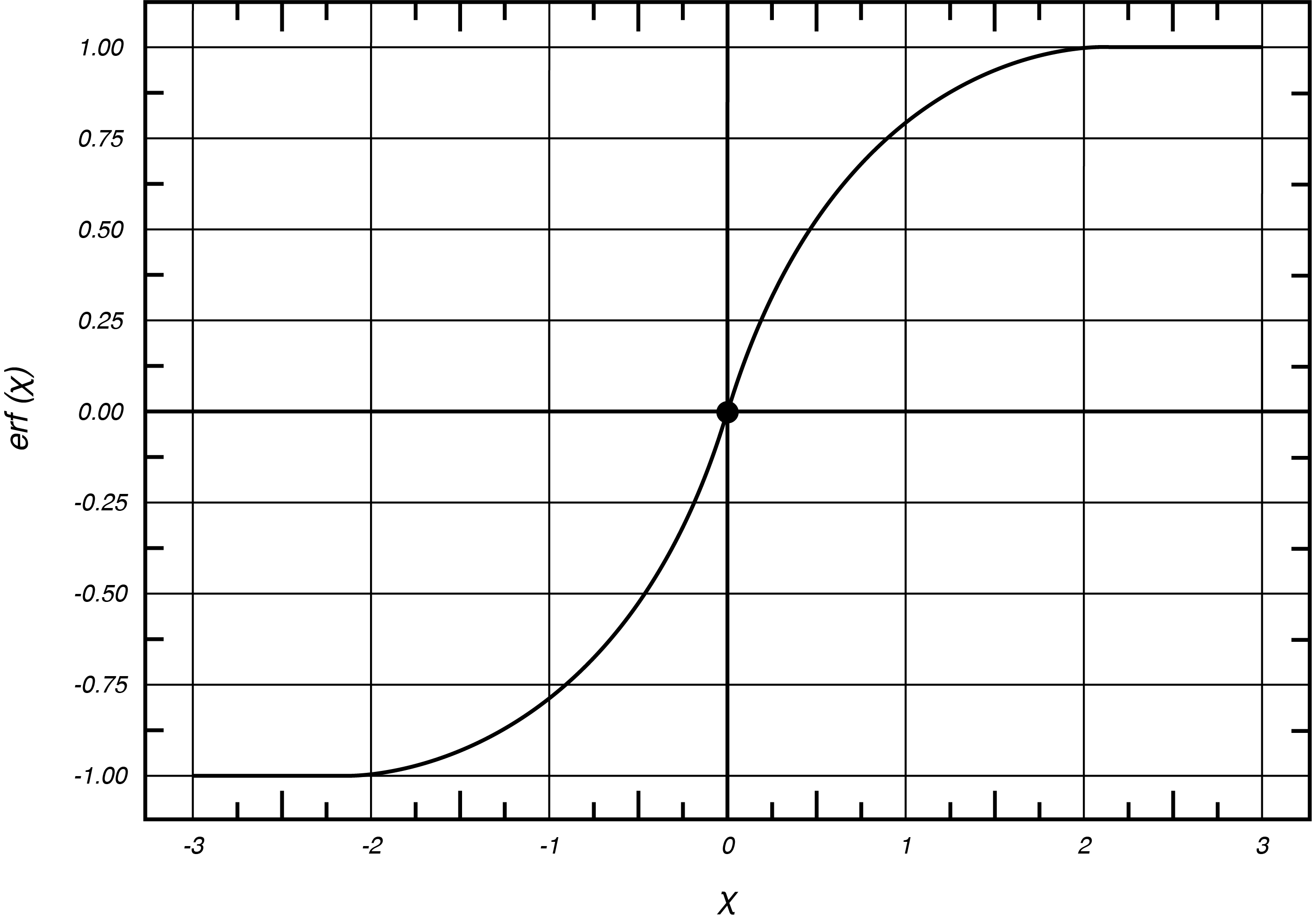
The first term on the right hand side is a straightforward integral evaluation up to a variable value [latex]\eta[/latex]. This can be replaced by the Gaussian Error Function, [latex]erf(\eta)[/latex] which is shown in Fig (7.6) as:
[latex]{erf \left(\eta \right)\ }=\frac{2}{\sqrt{\pi }}\int^{\eta }_0{e^{-{\eta }^2}d\eta }[/latex]
so that:
[latex]f=\frac{\sqrt{\pi }}{2}C_1{erf \left(\eta \right)\ }+C_2[/latex]
We are left to evaluate the constants from the two boundary conditions for f.
Since [latex]erf (0) = 0[/latex] and [latex]erf (\infty )=1[/latex] then [latex]C_1=-\frac{2}{\sqrt{\pi }} \text{ and } C_2 = 1[/latex] and the final form of the equation is:
[latex]f=\frac{u}{U }=1-erf(\eta) \text{ and } f' =-{\frac{2}{\sqrt{\pi}}e^-{^\eta}}^2\tag{7.32}[/latex]
The results of Eqn. (7.32) are plotted in Fig. 7.7. This solution is a “similarity solution” in that the results collapse, in this case, into a single variable, [latex]\eta[/latex], which depends on the two independent variables, [latex]x{}_{2}[/latex] and t. There are two parameters affecting the result of the local velocity, the boundary condition, [latex]U_p[/latex], and the fluid property, [latex]\nu[/latex]. To evaluate a given set of conditions one does the following. (1) Identify the physical space and boundary conditions of interest. (2) Transform variables such as values of space or time into associated values of the variable [latex]\eta[/latex]. (3) Use Eqn. (7.32) to determine the value of [latex]f[/latex] versus [latex]\eta[/latex] and the desired [latex]\eta[/latex] value. (4) Transform f into the desired velocity [latex]u[/latex].

Besides determining the local velocity in the fluid these results are also useful in determining the transient wall shear stress, or force per unit area of the plate. Given in Eqn. (7.32) is the derivative, [latex]f'[/latex]. This provides information of the velocity derivative, [latex]\frac{\partial u}{\partial x_2}[/latex]. Since there is only one velocity component and it is only a function of [latex]x{}_{2}[/latex] we can write the shear stress as:
[latex]\tau =\mu \left(\frac{\partial u_2}{\partial x_1}+\frac{\partial u_1}{\partial x_2}\right)=\mu \frac{\partial u_1}{\partial x_2}=\mu \left(\frac{Uf'}{2\sqrt{\nu t}}\right) \tag{7.33}[/latex]
where [latex]f'[/latex] is the derivative [latex]\frac{\partial f}{\partial \eta }[/latex]. The force on the surface of the plate with an area of LS, (where L is the distance along the plate in the direction of motion and S is the width, or span of the plate) due to its motion is:
[latex]F_p=\int^L_0{{\tau }_sdx_1S}\tag{7.34}[/latex]
where the shear stress, [latex]{\tau }_s[/latex], is evaluated at the surface where [latex]x{}_{2}[/latex] = 0. Evaluating (7.34) using (7.33) at [latex]\eta =0[/latex], with [latex]f'(0)=-\frac{2}{\sqrt{\pi } }[/latex] results in:
[latex]{\tau }_s=-\frac{\mu U_p}{\sqrt{\pi \nu t}}[/latex]
and the force
[latex]F_p=-\frac{\mu U_p LS}{\sqrt{\pi \nu t}}\tag{7.35}[/latex]
Notice that the wall stress decreases with time as momentum diffuses away from the surface. The force therefore also decreases with time. At time t = 0 the equations have a problem, since we said the acceleration was initially infinite.
We can define the diffusion distance way from the surface as the distance [latex]x{}_{2}[/latex] to where the velocity decays to 1% (small arbitrary value) of the plate velocity. So setting [latex]f[/latex] = 0.01 we see that [latex]\eta[/latex] = 1.85 and setting [latex]x_2=\delta[/latex] at this point we have:
[latex]\delta =3.7\sqrt{\nu t}\tag{7.36}[/latex]
Notice that the diffusion distance increases with time as well as kinematic viscosity. The greater the viscosity the further is the distance, [latex]\delta[/latex], at any given time. It is independent of the plate velocity.
One last item on this seemingly simple problem that will help in the interpretation of boundary layer flows. This flow has vorticity, but only aligned with the [latex]x{}_{3}[/latex] direction, as can be seen by calculating the local vorticity distribution:
[latex]{\omega }_3=\left(-\frac{\partial u}{\partial x_2}\right)=-\frac{Uf'}{2\sqrt{\nu t}}\tag{7.37}[/latex]
The circulation is the area integral of the vorticity, so extending an integration from the surface at [latex]x_2=0[/latex] to [latex]\delta[/latex], for a distance L along [latex]x{}_{1}[/latex], then the total circulation per distance [latex]x{}_{3}[/latex] becomes:
[latex]\Gamma=\int ^\delta_0 - \frac{U_p f'}{2 \sqrt{\nu t}} dx_2L= \int_{0}^{\infty }-U_p f'd \eta L=-U_p L[/latex]
where for [latex]x_2[/latex] greater than [latex]\delta[/latex] the value of [latex]f'[/latex] = 0 so there is no contribution to [latex]\Gamma[/latex].
Interestingly, the total circulation remains constant overtime, but the area grows since [latex]\delta[/latex] increases with time. The diffusion process merely spreads the vorticity over an increasing area, for increasing time and all of the vorticity is generated with the initial acceleration of the surface.
