X. Introduction to Turbulence Effects

The physical attributes of turbulent flow, in and of itself is a very difficult subject. That is to say, the flow characteristics of turbulence are difficult to measure, difficult to interpret and very difficult to incorporate into analyses. Never-the-less progress has been made, but much of it relies heavily on empirical results. Turbulence is typically described as a time varying phenomena of all dependent variables (except density for incompressible flows). In addition, spatial variations of the time dependency occurs as well. The results are that all of the velocity components and the pressure have spatio-temporal variations. Since the Navier-Stokes equations are nonlinear (through the convective acceleration terms) the statistical description of the flow relies on correlation functions among the various variables. There are a number of books written on the mathematical description of turbulence that can be challenging to incorporate into engineering applications. The nonlinear effects and some of the statistical measures of turbulence will become obvious once we look at the governing equations. For our purposes we will look at some of the physical consequences of turbulent flows and then illustrate how turbulent effects can be incorporated into an analysis of the viscous forces in boundary layer flows.

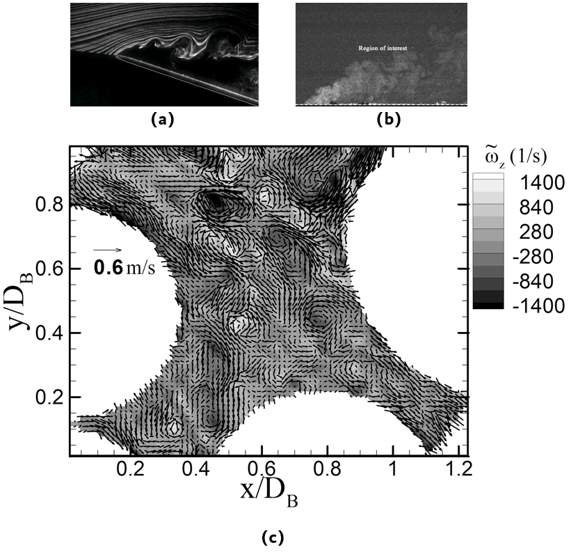
A few examples of turbulent flows are shown in Fig. 10.1. There are a wide range of fluctuations both in space and time. By scales we mean the magnitudes of local variations in time and space attributed to turbulent fluctuations about some local mean value. These are referred to as a broad spectrum of scales occurring within the flow. The flow geometry can have a large impact on the larger scales within the flow, since they interact often with the boundaries. However, the smaller scales tend to be mostly independent of the flow geometry indicating that there may be some underlying theoretical basis for their flow dynamics.

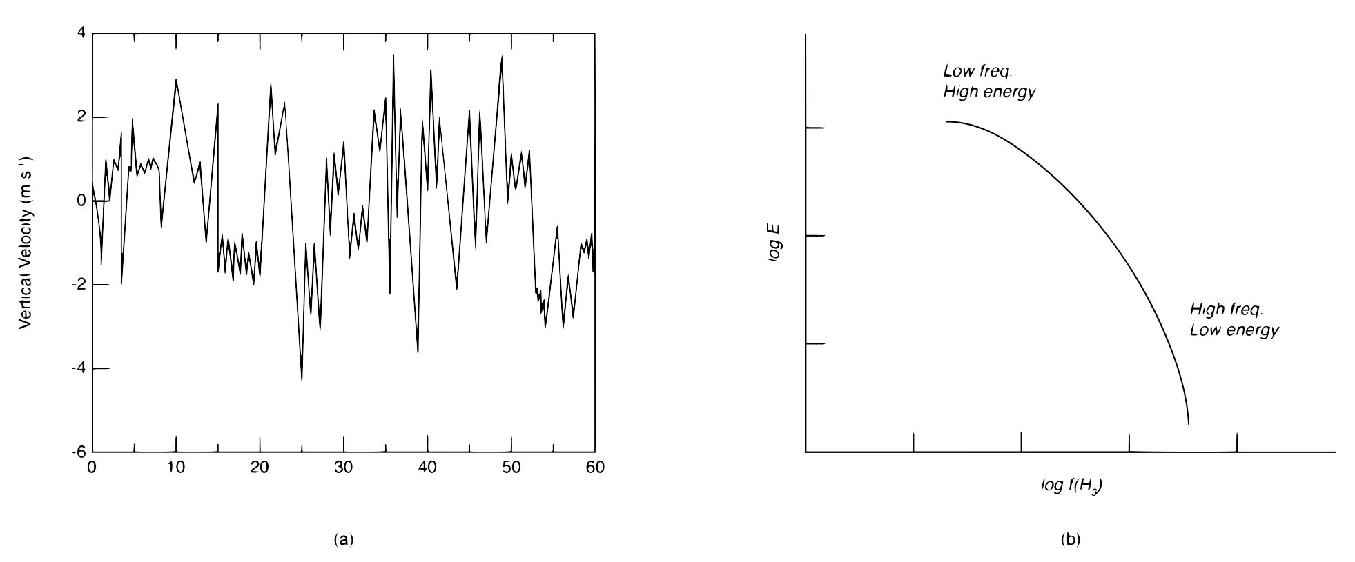
Shown in Fig. 10.2 is a typical time history signal of a measured velocity component say from a hot wire anemometer at a given location within the flow. Although this signal may seem random in nature, it has been learned that there is a lot of structure to these kinds of signals. One thing to notice is that there are time events happening over many different time scales. There are small scale (or short) events with relative small fluctuating values coupled with longer time varying, higher amplitude fluctuations. The short time events seem to be superimposed over the longer events. To help illustrate this variation of time scales Fig. 10.2 also illustrates the “energy spectrum” of the time series signal. Here the mean square value of the fluctuations are decomposed by using a Fourier transformation of the signal. The mean square fluctuations have units of velocity squared that can be interpreted as the kinetic energy per mass of fluid. This plot identifies the frequency dependency of the energy associated with the signal. We see that the larger amplitude fluctuations occur at the longer time scales (lower frequency) and the smaller amplitude fluctuations occur at the shorter time scales (higher frequency). Turbulent flows are characterized by a broad spectrum within the signal typically with large amplitude (or energy) fluctuations having low frequency and low amplitude high frequency components. Looking at Fig. 10.2 we see that the longer time scales have several orders of magnitude greater energy than the smallest scales. This distribution has implications concerning the mixing characteristics of turbulent flows such as in the ability to promote high reaction rates in combustion and other chemical reactions. In contrast the energy spectrum of a flow that has a single oscillating frequency would have an energy spectrum that would appear as a spike at the frequency of oscillation and would not be referred to as turbulent.

The integration of the energy spectrum over all frequencies yields the total energy of the fluctuations in the signal. This is equivalent to the time average of the square of the fluctuations (the mean square value) [latex]\overline{{u'}^2}[/latex], where the fluctuating velocity is [latex]u'=\left(u-\overline{u}\right)[/latex] with [latex]\overline{u}[/latex] being the time average value of the velocity and u is the instantaneous value of the velocity. This can be used to define the “turbulent intensity” as:

[latex]\frac{{\overline{\left({u'}^2\right)}}^{1/2}}{\overline{u}}[/latex] = “turbulent intensity”

Notice that [latex]\overline{{u'}^2}[/latex] is obtained for a single velocity component, say [latex]u_{1}[/latex], so this represents the turbulent intensity of one component. If we calculate the mean square value for each component the total energy, known as the turbulent kinetic energy (“tke”) is:

[latex]tke\ =\frac{1}{2}\ \left(\left(\overline{{{u'}_1}^2}\right)+\left(\overline{{{u'}_2}^2}\right)+\left(\overline{{{u'}_3}^2}\right)\right) \tag{10.1}[/latex]

The greater the tke typically the more intense is the turbulence. This measure of turbulence can be measured at each location within the flow to determine the spatial distribution of turbulence in a time averaged sense.

Reynolds Averaging

The concept of time averaging of the terms in the Navier-Stokes equation after the velocity is decomposed into a mean and time varying component is known as Reynolds averaging. The instantaneous velocity can be expressed as the sum of the fluctuating part and the mean value at any point in the flow as shown above an rewritten here slightly differently:

[latex]u=\left(u'+\overline{u}\right) \tag{10.2}[/latex]

where the primed quantity is the fluctuating value, which is time dependent, and [latex]\overline{u}[/latex] is the time average value. It should be noted that the time average of the fluctuating part is by definition zero. Each of the time dependent terms in the conservation of mass (or continuity equation) and Navier-Stokes equations can be replaced with the right hand side of Eqn. (10.2). Then each term is time averaged. For instance in the convective acceleration term:

[latex]\overline{u_j\frac{\partial u_i}{\partial x_j}}=\overline{\left({u_j}'+\overline{u_j}\right)\frac{\partial \left({u_i}'+\overline{u_i}\right)}{\partial x_j}}=\overline{{u_j}'\frac{\partial {u_i}'}{\partial x_j}}+\overline{u_j}\frac{\partial \overline{u_i}}{\partial x_j} \tag{10.3}[/latex]

Where the two terms containing products of the mean and fluctuating parts, when time averaged, are zero since the time average of the fluctuations in zero.

The last term in Eqn. (10.3) is merely the convective acceleration using the time average velocities. Notice that the time averaging and the spatial derivatives can be interchanged. The first term on the very right hand side is the time average of the convective acceleration of the fluctuating velocities. This term is not necessarily zero for a term consisting of the product of two or more time varying signals. This is because the average of the products of time varying signals is not equal to the product of the averages of those signals. Let’s examine this term a bit closer for incompressible flow we can write.

[latex]\overline{{u_j}'\frac{\partial {u_i}'}{\partial x_j}}=\frac{\partial \overline{\left({u_i}'{u_j}'\right)}}{\partial x_j} \tag{10.4}[/latex]

Where, for incompressible flow, we are able to bring the velocity [latex]u_j[/latex] inside the derivative with respect to [latex]x_j[/latex] from the continuity condition for incompressible flows. This term can be interpreted as the spatial derivative of the correlation function [latex]\left(\overline{{u_i}'{u_j}'}\right)[/latex] that is the time averaged product of the various velocity components. This is a second order tensor with six independent components since it is a symmetric tensor. This quantity, [latex]\left(\overline{{u_i}'{u_j}'}\right)[/latex] represents the contribution of turbulence to the mean momentum of the flow. That is to say, we have found a term that can change or adjust the mean momentum distribution in the flow caused by averaging the Reynolds decomposition of convective acceleration terms. We will see how this term affects the wall shear stress acting on the fluid for turbulent flow conditions.

Based on our earlier introduction of the turbulent kinetic energy, tke, one might expect that increased levels of tke would be associated with an increased magnitude of [latex]\left(\overline{{u_i}'{u_j}'}\right)[/latex] and increase the effect on the mean momentum distribution. How this occurs and under what conditions it occurs is not a simply thing to determine. This is because the relationship of the energy content of the fluid fluctuations with the momentum transport properties of the turbulence is a set of complicated interactions. Never the less it is possible to observe trends of these interactions and to formulate models of how they work.

We further manipulate the time averaged Navier-Stokes equations by bringing the new fluctuating term [latex]\left(\overline{{u_i}'{u_j}'}\right)[/latex] over to the right hand side of the equation and group it with the viscous stress term:

[latex]\rho \overline{u_j}\frac{\partial \overline{u_i}}{\partial x_j}=-\frac{\partial \overline{P}}{\partial x_j}+{\rho g}_i+\left(\frac{\partial }{\partial x_j}\left(\mu \frac{\partial \overline{u_i}}{\partial x_j}-\rho \left(\overline{{u_i}'{u_j}'}\right)\right)\right)\tag{10.5}[/latex]

Here we can see that the viscous term is combined with the momentum altering fluctuating term while all other terms are similar to the laminar flow equation except here we use the time average value of the variables. The last term has two contributions, the mean viscous stress term [latex]\ \mu \frac{\partial \overline{u_i}}{\partial x_j}[/latex], and the turbulence term. If we interprete the turbulence term as one that modifies the momentum distribution in the flow we can identify it as a “stress” and call it the “turbulent stress”, [latex]{\tau }_t[/latex] and write it as:

[latex]{\tau }_t=-\rho \left(\overline{{u_i}'{u_j}'}\right)\tag{10.6}[/latex]

In honor of Reynolds, who developed the Reynolds decomposition leading to this results this is often labeled the “Reynolds stress”. We can write the total stress within the flow as:

[latex]{\tau }_{total}={\tau }_{viscous}+{\tau }_{turbulent}=\ \mu \frac{\partial \overline{u_i}}{\partial x_j}-\rho \left(\overline{{u_i}'{u_j}'}\right)\tag{10.7}[/latex]

In a number of situations the viscous stress is actually a lot smaller than the turbulent stress and can be ignored except maybe in certain region of the flow, say near a surface or object where the fluctuating quantities are dampened.

Turbulent Boundary Layer

The discussion that follows assumes that the flow is turbulent over the entire surface. The conditions for this are discussed later after this section. Similarly to what was done in laminar flow turbulent boundary layer flows can be analyzed using the same assumptions used to simplify the governing equations. Basically we assume the following for a two dimensional boundary layer flow:

• thin boundary layer, [latex]\delta \ll[/latex] L (or x)
• stream-wise velocity greater than the cross-stream velocity, [latex]u_1\gg u_2[/latex]
• cross-stream derivatives greater than stream-wise derivatives, [latex]\frac{\partial }{\partial x_1}\ll \frac{\partial }{\partial x_2}[/latex]
• large [latex]Re{}_{x_1}[/latex]

The resulting time averaged governing momentum equation becomes for constant property flows and ignoring the body force term:

[latex]\rho \overline{u_1}\frac{\partial \overline{u_1}}{\partial x_1}\ \ \ \rho \overline{u_2}\frac{\partial \overline{u_1}}{\partial x_2}=-\frac{\partial \overline{P}}{\partial x_1}+\left(\frac{\partial }{\partial x_2}\left(\mu \frac{\partial \overline{u_1}}{\partial x_2}-\rho \left(\overline{{u_1}'{u_2}'}\right)\right)\right)\tag{10.8}[/latex]

Here we have retained the pressure gradient term and only the mean pressure value remains after time averaging the mean plus fluctuating parts.

Notice that in the Reynolds stress term the only contribution is from what is called the “cross correlation”, [latex]\rho \overline{{u_1}'{u_2}'}[/latex]. This is a consequence of [latex]\frac{\partial }{\partial x_1} \ll \frac{\partial }{\partial x_2}[/latex] even though [latex]\overline{u'_1 u'_1}[/latex] may be the same order of magnitude as [latex]\overline{u'_1 u'_2}[/latex].

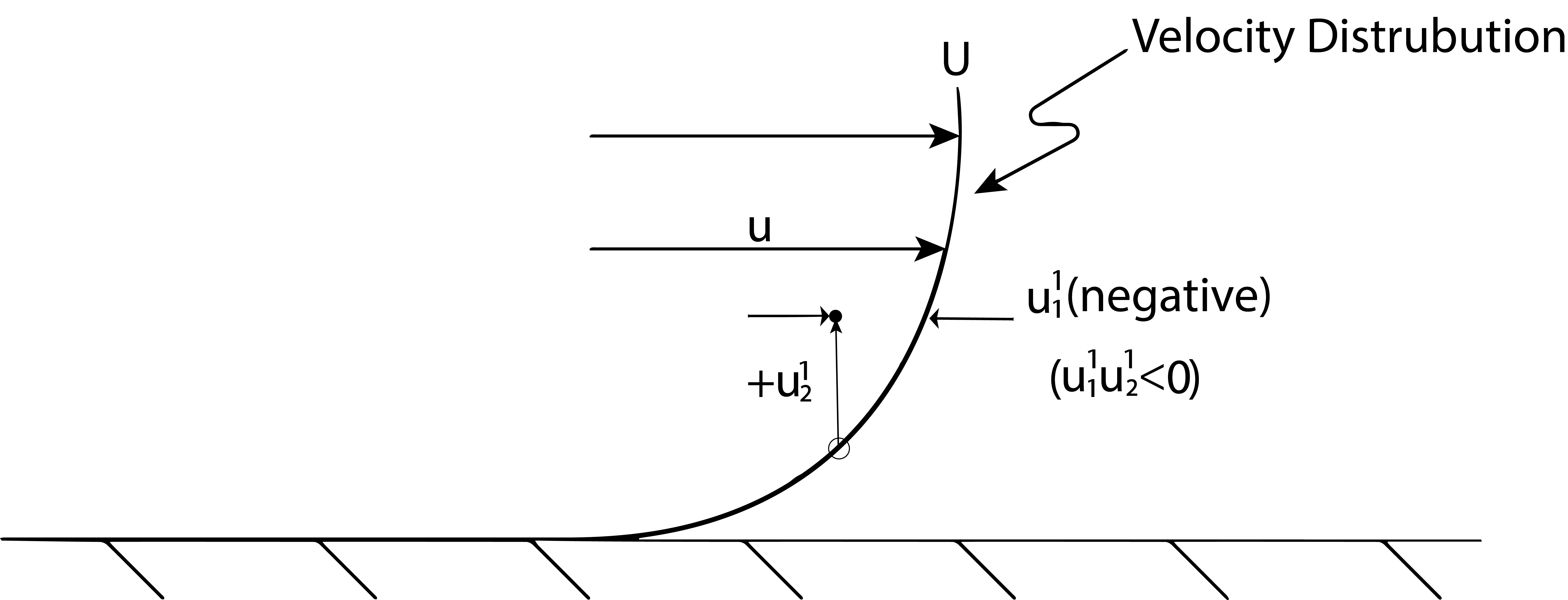
The effect on the mean momentum distribution, caused by turbulence, then is brought about by the cross correlation contained in the Reynolds stress. Referring to Fig. 10.3 we attempt to provide some rationale for how this correlation may impact the momentum distribution and consequently the wall shear stress. At an instant in time imagine a positive, upward value of [latex]u{}_{2}[/latex]. This moves fluid with a lower value of [latex]u{}_{1}[/latex] into a region of higher [latex]u{}_{1}[/latex] on average. Therefore the instantaneous value of [latex]{u_1}'{u_2}'[/latex] will be a negative number. Similarly if there is a negative value of [latex]u{}_{2}[/latex] it will move high [latex]u{}_{1}[/latex] velocity fluid into a slower moving region again causing [latex]{u_1}'{u_2}'[/latex] to be a negative number. Assuming this to be the case, one may assume that on average the value of [latex]\overline{{u_1}'{u_2}'\ }[/latex] is a negative number which means the added turbulent stress is positive, see Eqn. (10.6). This added stress slows down higher speed fluid and speeds up lower speed fluid. The result is a much flatter velocity or momentum distribution across the flow. However, the no-slip condition still holds true. This implies that on average the flatter velocity profile will have higher velocity gradients near the surface, such that the overall frictional force is larger. The net result is that a turbulent boundary layer is expected to have larger surface viscous stresses.

Scaling for Turbulent Boundary Layer Flows

We will define the displacement thickness, [latex]\delta _{1}[/latex], and the momentum thickness, [latex]\delta _{2,}[/latex] identically as before for laminar flow except we use the time average values of velocity. However, we need to determine an appropriate method to scale the velocity to arrive at an accurate velocity distribution. As for laminar flow we can define the nondimensional cross-stream coordinate as: [latex]\eta =\frac{x_2}{\delta }[/latex]. It turns out that the freestream velocity that was used to scale the stream-wise velocity in laminar flow may not be the best scale for the velocity within the boundary layer. The fairly flat velocity distribution of [latex]\overline{u_1}[/latex] in turbulent flow is heavily influenced by the velocity gradient near the wall that determines the wall shear stress. Consequently, a new velocity scale can be introduced that is proportional to the wall stress, called the “friction velocity”:

[latex]{v_f}=\sqrt{\frac{{\tau }_s}{\rho }}\tag{10.9}[/latex]

Notice that it is not a specific velocity within the flow but has units of velocity and is proportional to the velocity gradient at the surface through the value of the wall shear stress, [latex]\tau_s[/latex]. Since it is reasonable to note that the surface stress depends on the freestream velocity, one can also anticipate that [latex]{v_f}=f(U)[/latex].

From this we form the nondimensional velocity components:

[latex]{u_1}^+=\frac{\overline{u_1}}{{v_f}}\tag{10.10a}[/latex]

[latex]{u_2}^+=\frac{\overline{u_2}}{{v_f}}\tag{10.10b}[/latex]

As we will see in the next section, this scaling of velocity can be used to arrive at an accurate near wall velocity distribution in non-dimensional variables. However, if we choose to try to determine the wall shear stress using an integral analysis similar to what was done in laminar flow, then we can use the following. First we assume a functional form:

[latex]\frac{\overline{u_1}}{U}={f}{(\eta)}\tag{10.11}[/latex]

In contrast to the polynomial distribution we used in laminar flow. We assume a power law instead of the polynomial (since it has been shown to match experimental data well) as:

[latex]\frac{\overline{u_1}}{U}=\ {C\eta }^{1/n}\tag{10.12}[/latex]

where n is a positive integer and C is a constant. However, if we note that [latex]\frac{\overline{u_1}}{U}=1[/latex] at [latex]\eta[/latex] =1 then C = 1. Using this expression in the definitions for [latex]{\delta}_{1}[/latex] and [latex]{\delta}_{2}[/latex] we get:

[latex]\frac{{\delta }_1}{\delta }=\ \frac{1}{n+1}\tag{10.13}[/latex]

[latex]\frac{{\delta }_2}{\delta }=\ \frac{n}{\left(n+1\right)\left(n+2\right)}\tag{10.14}[/latex]

Experimental data shows that n is a weak function of Reynolds number, such that as Reynolds number increases the velocity profile becomes flatter and n increases. For moderately large Reynolds numbers n [latex]\mathrm{\sim}[/latex] 7 matches data very well.

To go any further with this we need a relationship between [latex]{\tau}_{s}[/latex] and [latex]\delta[/latex], similar to what was done with laminar flow, based on the nondimensional velocity distribution. For this we use an alternative scaling with a power law assumption given by:

[latex]{u_1}^+=f_2(\frac{x_2{v_f}}{\nu })=\ C_2{\left(\frac{x_2{v_f}}{\nu }\right)\ }^{1/n} \tag{10.15}[/latex]

where [latex]C{}_{2}[/latex] is a constant and [latex]\frac{\nu}{v_f}[/latex] is a new length scale. At [latex]x{}_{2} = \delta[/latex], we know that [latex]\frac{\overline{u_1}}{U}=1[/latex] so we can write:

[latex]\frac{U}{{v_f}}=\ C_2{\left(\frac{\delta {v_f}}{\nu }\right)\ }^{1/n} \tag{10.16}[/latex]

This provides the relationship between [latex]{\tau}_{s}[/latex] and [latex]\delta[/latex], since [latex]{\tau}_{s}[/latex] is contained in [latex]{v_f}[/latex], see Eqn. (10.9). After inserting the definition of [latex]{v_f}[/latex] and a little algebra we obtain:

[latex]\frac{{\tau }_s}{\rho U^2}={C_2}^{-\frac{2n}{n+1}}{Re_{\delta }}^{-\frac{2}{n+1}} \tag{10.17}[/latex]

where [latex]Re_{\delta }=\frac{U\delta }{\nu }[/latex] which represents a Reynolds number based on the boundary layer thickness.

Now we use the momentum integral equation that was derived for laminar flow, which is also valid for turbulent flow that yields for a flat plate:

[latex]c_f=2\frac{{\delta }_2}{\delta }\frac{d\delta }{dx_1}=\frac{{\tau }_s}{\frac{1}{2}\rho U^2}\tag{10.18}[/latex]

Noting that [latex]\ \frac{{\delta }_2}{\delta }[/latex] is a constant for a given value of n, and eliminating [latex]\tau_s[/latex] between Eqn. (10.17) and (10.18) and solving for [latex]\delta[/latex] we obtain:

[latex]\frac{\delta }{x_1}=\ C_T{Re_{x_1}}^{-\frac{2}{\left(n+3\right)}} \tag{10.19}[/latex]

where

[latex]C_T={\left[\frac{{{\left(\frac{n+3}{n+1}\right)C}_2}^{\frac{-2n}{n+1}}}{{{\delta }_2}/{{\delta }}}\right]}^{\frac{n+1}{n+3}}[/latex]

that is fully determined by the constant [latex]C{}_{2}[/latex] and the value of n. Based on experimental data, much of it analyzed by Blasius for turbulent flow results in:

[latex]C_2=8.74 \tag{10.20}[/latex]

Now we have Eqn. (10.19) fully determined so that we can find the derivative [latex]\frac{d\delta }{dx_1}[/latex] and inserts this into the expression for the skin friction, Eqn. (10.18). For the case of [latex]n = 7[/latex] we have:

[latex]C_T=0.37[/latex]
[latex]\frac{{\delta }_2}{x_1}=\ 0.036\ {Re_{x_1}}^{-1/5}[/latex]
[latex]c_f=\ 0.0577\ {Re_{x_1}}^{-1/5} \tag{10.21}[/latex]

The determination of the total viscous drag force acting on the surface of length L and width S is obtained exactly as was done for laminar flow, by integration of the surface shear stress over the area. The results for the case of [latex]n = 7[/latex]

[latex]C_f = \ 0.072\ {Re_L}^{-1/5} \tag{10.22}[/latex]

[latex]F_D=C_f\frac{1}{2}\rho U^2LS \tag{10.23}[/latex]

Initial Laminar Starting Length

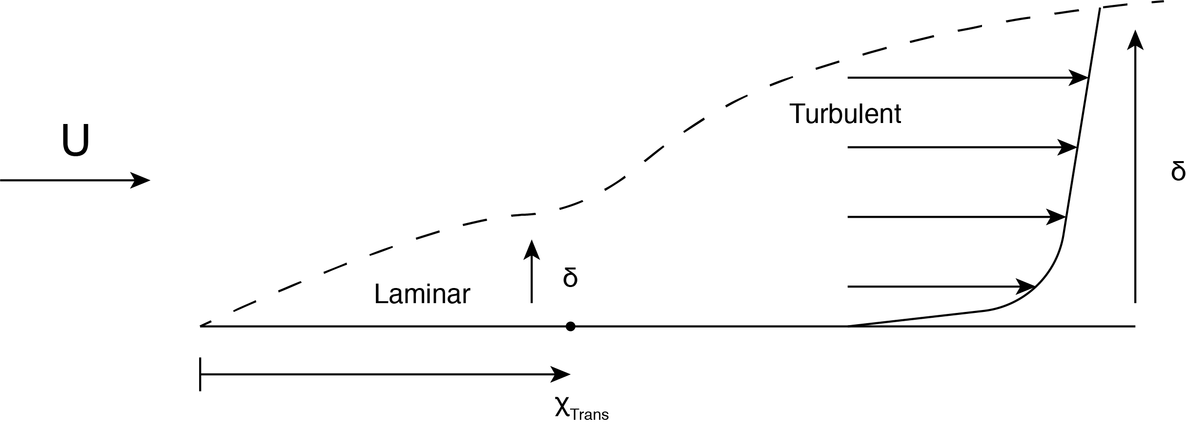
Turbulent flow over a surface in general will NOT exist from the beginning of the surface, [latex]x{}_{1}[/latex] = 0. Experiments haves shown that turbulent flow on a smooth surface occurs when the Reynolds number, [latex]Re{}_{x_1}[/latex], is greater than 5×10⁵. Since the Reynolds number is identically zero at the leading edge when [latex]x{}_{1}[/latex] = 0, there will be a region near the leading edge where laminar flow occurs, and then further along the surface the flow becomes turbulent if [latex]Re_{x_1}[/latex] is large enough. Turbulent flow can occur from, or very close to, the leading edge if the flow is tripped. This occurs when there may be slight roughness near the leading edge and the freestream velocity is sufficiently large that turbulence occurs. Under these conditions the Eqns. (10.22) and (10.23) are valid over the entire length of the flow. For the conditions when the flow is not tripped the laminar starting region needs to be considered. A sketch of the boundary layer thickness as influenced by the initial laminar starting length and the transition to turbulence is shown in Fig. 10.4.

The solution to this situation of laminar flow up to the transition location along the surface and turbulent flow beyond this is obtained by dividing up the integration of the surface shear stress into laminar and turbulent regions. The location dividing the two regions is where [latex]x = x _{transition}[/latex] which is found using the critical Reynolds number.

[latex]x_{transition}=\frac{\left(5x10^5\right)\nu }{U} \tag{10.24}[/latex]

Once the transition location is found then the integration over the entire surface becomes:

[latex]F_D=\int^{x_{transition}}_o{{\tau }_sdx_1\ S}\ +\int^L_{x_{transition}}{{\tau }_sdx_1 S} \tag{10.25}[/latex]

Each term is now divided by [latex]\frac{1}{2}\rho {U_{\infty }}^2(LS)[/latex] to convert this equation into a nondimensional equation for [latex]C{}_{D}[/latex]. The integrand for each term will be the skin friction coefficient, [latex]c{}_{f}[/latex] and [latex]dx{}_{1}[/latex] becomes [latex]d(x/L)[/latex]. There is a problem here though, the expression for [latex]c{}_{f}[/latex] for the turbulent part (the second integral) can not be solved directly because the skin friction expression found previously assumes the flow begins turbulent at the leading edge. The solution to this problem is to recast the above integral by adding and subtracting the contribution to the total force from [latex]x = 0[/latex] to [latex]x = x{}_{transition}[/latex] based on turbulent flow. When this is added to the second term in Equation (10.25) the result is an expression for the force assuming turbulent flow from [latex]x = 0[/latex]. The subtraction of this term in the first integral results in the difference between the laminar and turbulent generated force up until [latex]x_{transition}[/latex]. Rearranging the terms results in

[latex]C_D=\ \int^L_0{c_{f,\ turbulent}d\left(\frac{x}{L}\right)}-\int^{x_{transition}}_o{\left(c_{f,\ turbulent}-c_{f,\ laminar}\right)d\left(\frac{x}{L}\right)} \tag{10.26}[/latex]

By using the transitional location given in Eqn. (10.24) the second integral in Eqn. (10.26) can be found directly using the expressions for [latex]c{}_{f}[/latex]. Writing this using [latex]Re{}_{L}[/latex] (the Reynolds number evaluated at the end of the surface) results in:

[latex]C_D=\ \frac{0.072}{{Re_L}^{1/5}}-\frac{1700}{Re_L} \tag{10.27}[/latex]

It should be noted that the above expression assumes [latex]n = 7[/latex]. Also, if transition occurs at a slightly different Reynolds number the coefficient in the numerator of the second term in this equation will vary. The numerator of the second term may differ slightly based on the selected critical Reynolds number or power law exponent used.

Universal Velocity Profile

We now introduce the concept of the logarithm velocity profile in the near wall region of a turbulent boundary layer. This concept has proven to match experimental data very well and it is based on the premise that very close to the wall there is a constant shear layer. It also introduces the concept of a turbulent effective viscosity. If we take the stress term in the Navier-Stokes equation, Eqn. (10.7) for a boundary layer as:

[latex]{\tau }_{total\ }=\mu \frac{\partial \overline{u_1}}{\partial x_2}-\rho \left(\overline{{u_1}'{u_2}'}\right) \tag{10.28}[/latex]

We assume that this stress is a constant which can be written in terms of the friction velocity, [latex]{v_f}[/latex]. Then we model this term based on an effective viscosity, [latex]{\nu }_t[/latex], that accounts for both the viscous and turbulent contributions which results in the total stress in terms of the friction velocity as:

[latex]\frac{{\tau }_{total\ }}{\rho }=\ {{v_f}}^2={\nu }_t\frac{\partial \overline{u_1}}{\partial x_2} \tag{10.29}[/latex]

The effective viscosity (written here as a kinematic viscosity) has units of velocity times length. Taking the friction velocity as the appropriate velocity scale and [latex]x{}_{2}[/latex] as the appropriate length scale (since the viscous effects can only extend away from the wall some amount [latex]x{}_{2}[/latex]) then we model the effective viscosity as:

[latex]{\nu }_t=\kappa {v_f}x_2 \tag{10.30}[/latex]

where [latex]\kappa[/latex] is an unknown constant. Inserting Eqn. (10.30) into (10.29) we have:

[latex]{{v_f}}^2=\kappa {v_f}x_2\frac{\partial \overline{u_1}}{\partial x_2} \tag{10.31x}[/latex]

This is now integrated in the [latex]x_2[/latex] direction for a constant value of [latex]{v_f}[/latex] to obtain a velocity profile as:

[latex]\frac{\overline{u_1}}{{v_f}}=\frac{1}{\kappa }ln\ x_2+c \tag{10.32}[/latex]

This can easily be transformed into the following:

[latex]\frac{\overline{u_1}}{{v_f}}=\frac{1}{\kappa }ln\ \frac{x_2{v_f}}{\nu }+B \tag{10.33}[/latex]

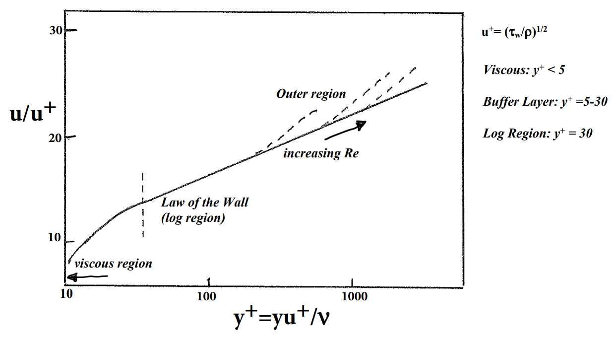
where [latex]\kappa[/latex] and B are constants determined from experimental results and shown to be [latex]\kappa =0.41[/latex] and B = 5. Actually there are also theoretical arguments that can be made to show that [latex]\kappa =0.41[/latex]. This constant stress layer result is only valid fairly close to the surface, but has been shown over a wide range of conditions (different fluids, different Reynolds numbers, etc.) to be very accurate. The non-dimensional variable, [latex]\frac{x_2{v_f}}{\nu }[/latex], is often given the symbol [latex]{x_2}^+\ or\ y^+[/latex], and [latex]\frac{\overline{u_1}}{{v_f}}=u^+[/latex], resulting in a non-dimensional velocity profile valid close to the wall that is expressed in terms of the wall shear stress contained in the variable [latex]u^+[/latex] and [latex]x_2^+[/latex].

This relationship for boundary layer flow of [latex]u^+[/latex] versus [latex]y^+[/latex] is shown in the figure below. Note that the region in which there is a log profile extends from approximately [latex]x_2^+=30[/latex] until the outer flow region is reached. The outer flow region is shown as a dashed line and begins further and further away from the wall (greater values of [latex]x_2^+[/latex]) with increasing Reynolds numbers. Close to the wall ([latex]x_2^+<30[/latex]) the turbulence is greatly suppressed by the wall and the log-profile is no longer valid. For [latex]x_2^+=0-5[/latex] the flow is dominated by viscous forces and it can be shown that [latex]u^+=y^+[/latex] (a linear velocity profile). Pressure gradients along the wall are known to effect the outer region primarily.