V. Potential Flows
In this chapter we will introduce a number of “basic ideal flows”. These flows will form a basis from which we can construct more complex flows. The basic principle we are relying on is “superposition”. This allows the linear addition of various flows that then result in more complicated flows. This is possible because the basic underlying equations that govern the flows are linear.
We have shown that there is an orthogonal relationship that exists between two variables that describe the flow, streamfunction and velocity potential, for ideal (irrotational and incompressible with zero viscous forces) flows. The orthogonal condition indicates that if we know one of these it is rather straight-forward to determine the other. We will use both of these flow descriptors to some extend, but mostly use the streamfunction representation of the various flows that we will consider. We will also restrict our results to two dimensional cases, although this is not necessary in general. Our basic equations are the Laplace equations we found in the previous chapter for the streamfunction, [latex]{\psi}[/latex], and velocity potential, [latex]{\phi}[/latex].
For ideal flows we have the simplified continuity equation that treats the density as a constant, and allows the elimination of the density directly in the equation. This results in a relationship among the velocity components that must hold true to satisfy conservation of mass. Also, the irrotational flow condition requires the vorticity to be zero which leads to additional conditions on velocity derivatives within the flow. The boundary conditions need to be specified for such flows, and are required to solve the governing equations. Since these flows are inviscid we do not have the no-slip boundary condition to help specify the value of the velocity. This implies that the velocity may be some (finite) value at a surface, not equal to the surface velocity). However, we can require that a surface be impermeable, that is no flow crosses the boundary. This then assures that the component of the velocity normal to the surface must be zero. So at least we can say something quantitative about a velocity component.
Basic Flows
In this section we present the governing equations for several basic flows. These equations are solutions of the Laplace equation and are determined through required boundary or imposed flow conditions. We deal with steady two dimensional flows.
Uniform Flow
The most simple flow (other than zero flow) is a steady uniform flow. This condition is a constant velocity in a given direction such that the velocity vector does not vary spatially. We designate this velocity as [latex]{U}[/latex]. If we align our coordinate system along the direction of [latex]{U}[/latex], such that [latex]{x{}_{1}}[/latex] is the direction of [latex]{U}[/latex], then there is only one nonzero velocity component. The streamfunction would be expected to be a straight line along the direction of [latex]{U}[/latex] as well. Using the definition of [latex]{\psi}[/latex] we obtain the following:
[latex]u=U=\frac{\partial \psi }{\partial x_2}[/latex]
Integrating this in [latex]{x{}_{2}}[/latex] we obtain an expression for the streamfunction:
[latex]\psi =Ux_2+f(x_1)[/latex]
But since
[latex]v=0=-\frac{\partial \psi }{\partial x_1}[/latex]
then [latex]{\psi}[/latex] is not a function of [latex]{x{}_{1}}[/latex] and we obtain
[latex]\psi =Ux_2+C\tag{5.1}[/latex]
We can arbitrarily set [latex]\psi = 0[/latex] at [latex]{x{}_{2} = 0}[/latex] so that
[latex]\psi =Ux_2\tag{5.2}[/latex]
If we proceed along the same line to solve for [latex]{\phi}[/latex] from its definition relative to the partial velocity derivative, Eqn. (4.1), the result is:
[latex]\phi =Ux_1\tag{5.3}[/latex]
where we have set [latex]{\phi}= 0[/latex] at [latex]{x{}_{1}} = 0[/latex], other wise there is an additive constant which is equal to the potential at [latex]{x{}_{1}} = 0[/latex].
For a condition of uniform flow, again with velocity of U, but at some angle [latex]{\alpha }[/latex] to the [latex]{x{}_{1}}[/latex] axis we have the following (the reader is encouraged to obtain this result by integrating the definition of the streamfunction):
[latex]\psi =U\left(x_2cos\alpha -x_1sin\alpha \right)+C\tag{5.4}[/latex]
The constant C is determined by a “datum” value of [latex]{\psi}[/latex] that passes through some point. For instance if [latex]\psi =0[/latex] at [latex](0,0)[/latex] then [latex]{C }= 0[/latex].
Going back to uniform flow (two dimensional) aligned in the [latex]{x_{1}}[/latex] direction we can find the volumetric flow rate per depth through some area say between [latex]{x{}_{2}} = 0[/latex] and [latex]{x{}_{2}}= 4[/latex] as:
[latex]\dot{Q}{'}[/latex] = [latex]\Delta \psi =U(4-0)=4U[/latex]
Source/Sink Flow
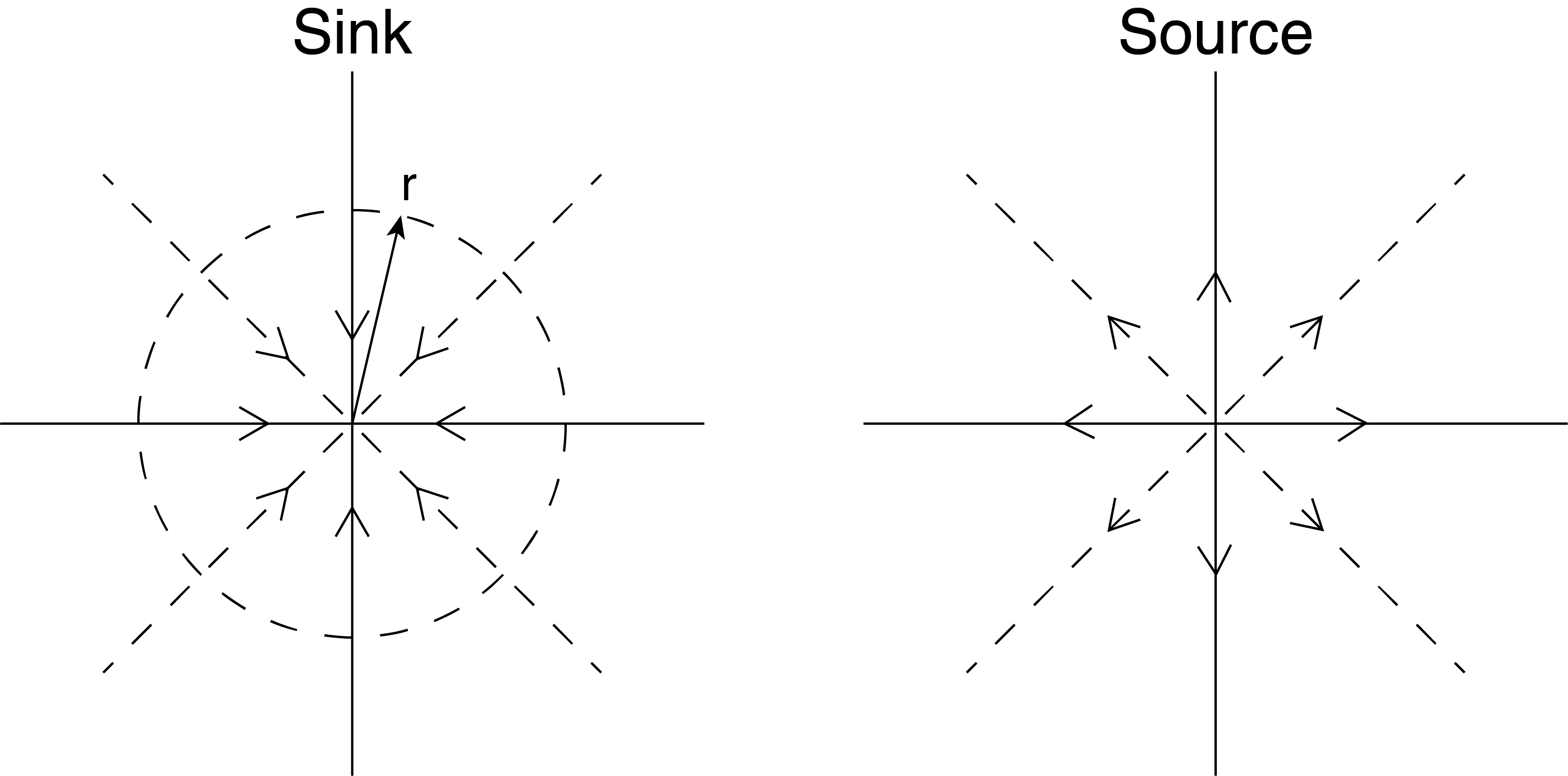
In two dimensional flow a source or a sink of flow is possible, since it implies that flow enters or leaves a given two dimensional plane. We treat this as a rate of gain (source) or loss (sink) of mass at some point within the flow. An example of this might be a simulation of a drain say in a tank with a flat bottom. Along the bottom plane flow leaves the plane of the bottom at a small opening. Here we shrink the size of the opening to a point (which is hard to imagine since we have mass flow rate through this point, since the velocity associated with this point is infinite across the plane). Despite these unrealistic characteristics, if we move away from this “singularity” point of infinite velocity and zero area we can assign a flow rate. This is illustrated in Fig. 5.1, which illustrates how flow approaches the sink along the plane with velocity vectors that are inwardly, straight radial streamlines, as shown as vector lines in Fig. 5.1.
By drawing a circle of an arbitrary radius, r, shown as the dashed line in Fig. 5.1, the flow rate is determined by integrating the velocity around the circle. This is because the circle represents the flow area (per unit depth into the page), and the velocity vectors are each normal to the circle based on symmetry. The result for the mass flow rate per unit depth into the page is:
[latex]\dot{m}{'}=\rho v_r2\pi r[/latex]
Note that [latex]v_r[/latex] is negative for a sink and positive for a source.
If a larger circle is drawn the same mass flow rate occurs into the point, but since the area is larger the velocity at the new larger circle is less. One can solve for the velocity, [latex]v_r[/latex], at any radial position, [latex]{r}[/latex], as:
[latex]v_r=\frac{\dot{m}{'}}{2\pi \rho }\frac{1}{r}=\frac{\dot{Q}{'}}{2\pi }\frac{1}{r}\tag{5.5}[/latex]
For a constant steady volumetric flow, [latex]\dot{Q}{'}[/latex], we see that the velocity decreases linearly as [latex]{ r}[/latex] increases. So this flow has straight streamlines all represented as radial lines from the center point. We see how the velocity increases rapidly in magnitude as [latex]{ r}[/latex] goes to zero, at which point it becomes infinite (or undefined). Based on the orthogonal condition between the velocity potential and streamfunction we see that lines of constant potential are circles (like the dashed line shown in Fig. 5.1.)
We can combine the constants in Eqn. (5.5) [latex]{\mu }_s=\frac{\dot{Q}{'}}{2\pi }[/latex], where [latex]{{\mu}_{s}}[/latex] is the “source strength” with units of [latex]m{}^{2}/s[/latex] in SI units such that:
[latex]v_{r,source}=\frac{{\mu }_s}{r}\tag{5.6}[/latex]
Eqn. (5.6) represents the flow from a source with strength [latex]{{\mu}_{s}}[/latex]. The source pumps fluid into the plane of flow with streamlines that are radially outward.
The flow can be reversed such that the flow along the radial lines is inward. This implies flow is exiting the plane, and this is a “sink”, with velocity inward, which has a negative [latex]{r }[/latex]component:
[latex]v_{r,sink}=-\frac{{\mu }_s}{r}\tag{5.7}[/latex]
The streamfunction is found by integrating the velocity based on the definition of the streamfunction using cylindrical coordinates:
[latex]v_r=\frac{\partial \psi }{r\partial \theta }=\frac{{\mu }_r}{r}[/latex]
[latex]\psi ={\mu }_s\theta\tag{5.8}[/latex]
Velocity potential lines are found from the definition of the potential relative to the velocity:
[latex]v_r=\frac{\partial \phi }{\partial r}=\frac{{\mu }_s}{r}[/latex]
Integrating this results in:
[latex]\phi ={\mu }_sln\ r\tag{5.9}[/latex]
Vortex Flow
Now consider a swirling flow such that the streamlines are circles. This implies that there is no radial velocity component, only [latex]v_{\theta }[/latex]. We label this swirling flow as a “vortex”, often called a “free vortex” since it is free from external forcing. It is also irrotational. If streamlines are circles as is shown in Fig. 5.2 then velocity potential lines must be straight radial lines from the center of the circle to be orthogonal to the streamlines.
To construct a flow with the above characteristics we examine the possible flow in cylindrical coordinates. Here we use the definition of the streamfunction in cylindrical coordinates:
[latex]v_{\theta }=-\frac{\partial \psi }{\partial r}[/latex]
[latex]{\omega }_z=0=\frac{\partial \left(rv_{\theta }\right)}{\partial r}[/latex]
So if we consider the flow to be given by its velocity [latex]v_{\theta }=c/r[/latex], where [latex]{C}[/latex] is a constant, then the vorticity will be zero as required. Inserting this into the definition for the streamfunction above yields:
[latex]\psi =-Cln\ r\tag{5.10}[/latex]
Next we define the “circulation” [latex]\mathrm{\Gamma }[/latex], as the line integral of the velocity around a closed line, or a loop, as:
[latex]\mathrm{\Gamma }\mathrm{=}\oint{v_{\theta }ds}\tag{5.11}[/latex]
This has units of [latex]m{}^{2}/s[/latex] in SI units. Inserting the expression for [latex]v_{\theta }[/latex] above and noting that [latex]ds=rd\theta[/latex] with the integration carried out between 0 and 2[latex]{\pi}[/latex], we get:
[latex]\mathrm{\Gamma }{=}\oint{v_{\theta }ds}=2\pi C \tag{5.12}[/latex]
The result is that the circulation within the vortex is a constant that can be determined knowing [latex]{C}[/latex]. We can replace C with [latex]{rv}_{\theta }[/latex] and solve for the velocity as:
[latex]v_{\theta }=\frac{\mathrm{\Gamma }}{2\pi r}=\frac{{\mu }_v}{r} \tag{5.13}[/latex]
where we define the “vortex strength” as:
[latex]{\mu }_v=\frac{\mathrm{\Gamma }}{2\pi }\tag{5.14}[/latex]
And also using the definition of vorticity, which must be zero to be irrotational, as:
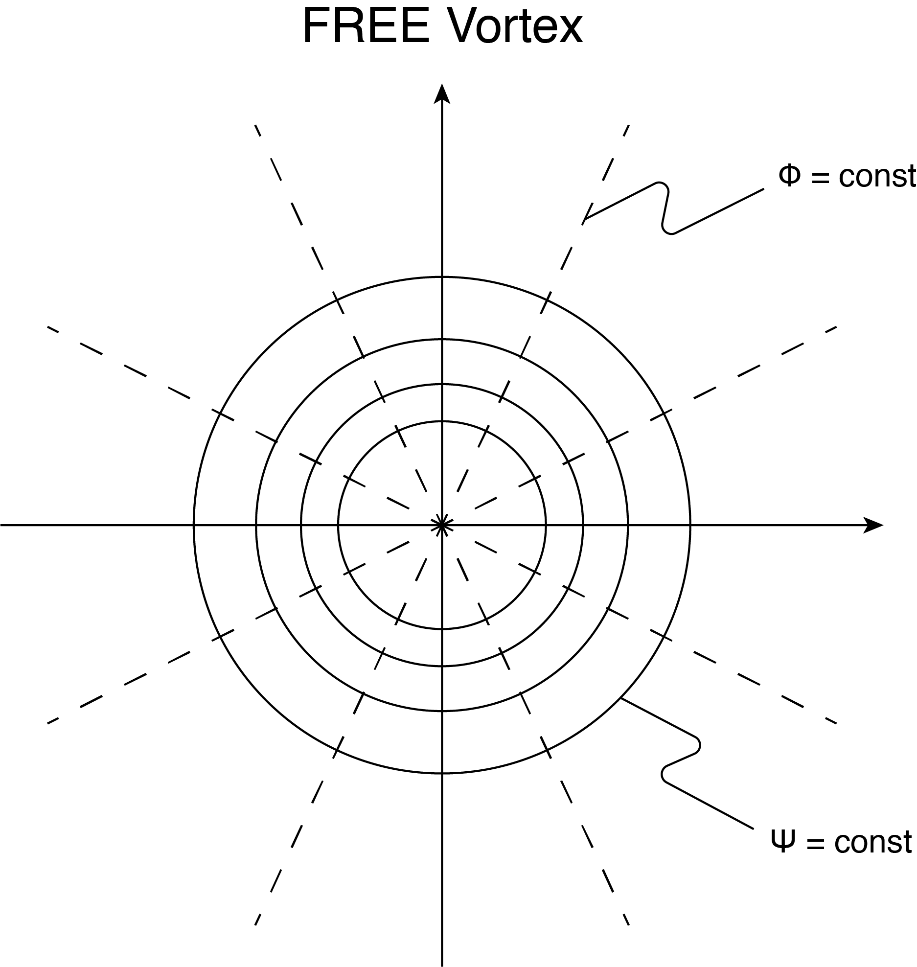
The flow for a free vortex is shown in Fig. 5.2 indicating streamlines as circles and the velocity potential as straight radial lines. Notice that theses lines are just the inverse of what we found for the source.
Since streamlines can have the velocity direction either counterclockwise or clockwise and still have the same general form with the same equations as shown above the sign convention is that a counterclockwise rotation is positive, and a clockwise rotation is negative. This is expressed in the value of [latex]{\Gamma},[/latex] or [latex]{\mu}_{s}[/latex]. In other words counterclockwise flow has positive circulation.
One last interesting aspect of the free vortex and the circulation is as follows. We use the vector identity:
[latex]\int{\left(\mathrm{\nabla }\times \boldsymbol{V}\right)dA=\oint{\boldsymbol{V}\cdot d\boldsymbol{s}}}[/latex]
where [latex]\boldsymbol{V}[/latex] is any vector, [latex]{dA}[/latex] is an area and [latex]{d}\textbf{s}[/latex] is the vector distance along a closed loop integration around the area [latex]{A}[/latex]. If we let [latex]\boldsymbol{V}[/latex] be the velocity and noting that the vorticity is [latex]\boldsymbol{\omega }=\left(\mathrm{\nabla }\times \boldsymbol{V}\right)[/latex] and that the loop line integral is the circulation given above, then we can see that:
[latex]\mathrm{\Gamma }\mathrm{=}\oint{v_{\theta }ds}=\int{\boldsymbol{\omega }dA}\tag{5.15}[/latex]
Consequently the circulation is the area integral of the vorticity in some selected area within the flow. Note that we are dealing with a two dimensional flow and dA is within the plane of the flow so the vorticity is aligned along a vector out of the plane.
Now we have a bit of a dilemma. A free vortex has finite values of velocity [latex]v_{\theta }[/latex] that result is a certain circulation. This circulation is proportional to the vorticity within the flow. But we have said that the flow is irrotational, which means that the vorticity is zero. How can the circulation be nonzero while the vorticity is zero? The answer is that the vorticity (that drives the circular velocity) is concentrated at the center of the circle. Away from the center of the circle we know the vorticity is zero since the velocity we are using, [latex]v_\theta[/latex], was based on the vorticity being zero. If one calculates the circulation about a circular loop of radius [latex]r{}_{1}[/latex] (an area of [latex]\pi r{}_{1}{}^{2}[/latex]) and then repeats this calculation for a larger area of radius [latex]r{}_{2}[/latex], the result will be the same. This shows that in the area between [latex]r{}_{1}[/latex] and [latex]r{}_{2}[/latex] there is no added vorticity since the circulation remains the same. This can be done for any arbitrarily small radius [latex]r{}_{1}[/latex], showing that in the limit of r going to zero there is no vorticity within the flow except at r=0. A free vortex has a concentration of vorticity at r = 0. Also, the velocity must go to infinity, a velocity singularity. Interestingly this says that we can have isolated vorticity concentrations within an otherwise irrotational flow field.
Superposition
As stated previously superposition is a powerful tool that allows us to construct more complex flows from several simple flows. This is possible since the governing equation for the streamfunction, that describes streamlines, and the velocity potential are linear, is the Laplace equation.
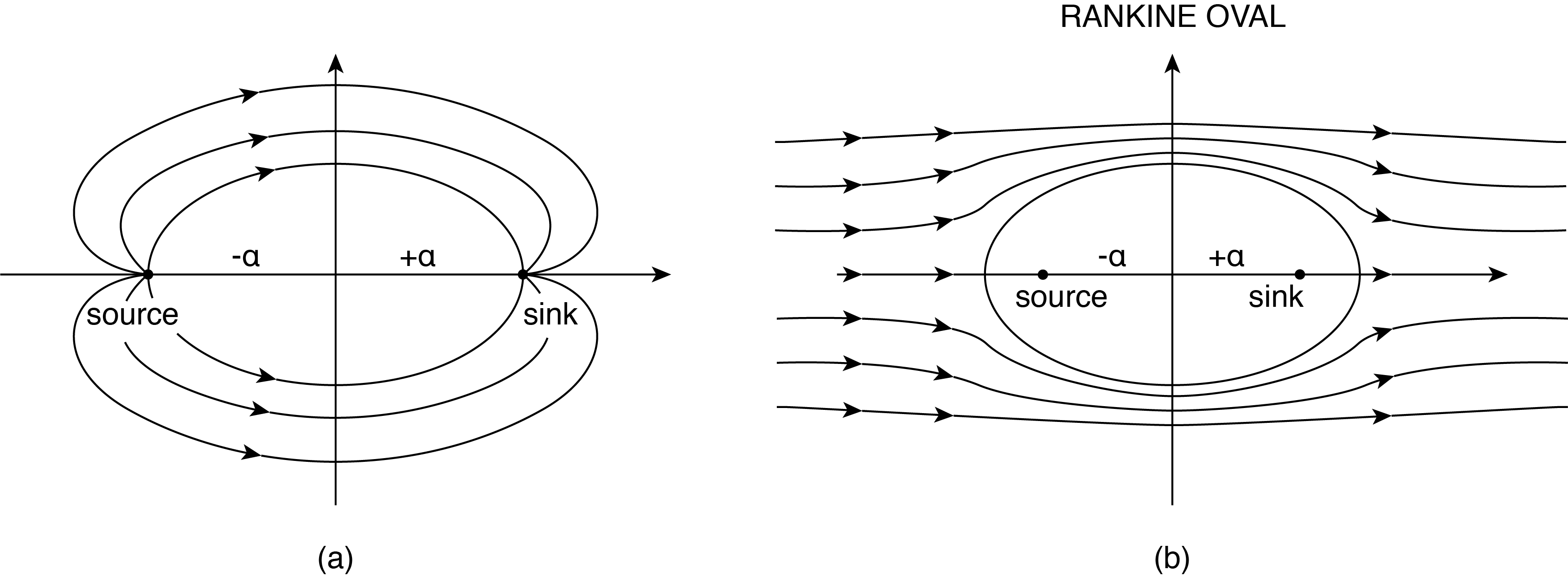
We begin by examining the flow field in the vicinity of a source and sink. We place the source and sink on the [latex]{x{}_{1}}[/latex] axis separated by distance 2a, as is shown in Fig 5.3 (a), with the origin mid way between each. The source is on the left (negative [latex]{x{}_{1}}[/latex], and the sink is on the right (positive [latex]{x{}_{1}}[/latex]). The streamfunction,or the velocity potential, at any point in the flow can be obtained by added together the streamfunction, or velocity potential, from the source plus that for the sink. However, care must be taken into account since our previously obtained equations were written assuming the source/sink were located at the origin of our coordinate system. In this case they are shifted along the [latex]x_1[/latex] axis. The result for any point P, located at ([latex]{x{}_{1},x{}_{2}}[/latex]) in the flow at distance [latex]r{}_{1}[/latex] and [latex]r{}_{2}[/latex]from the sink and source, respectively is:
[latex]\psi ={\psi }_{source}+{\psi }_{sink}[/latex]
[latex]\psi ={\mu }_s{\theta }_1-{\mu }_s{\theta }_2 \tag{5.16}[/latex]
where it is assumed the source and sink have equal but opposite strength and the angles are shown in Fig. 5.3. Similarly for the velocity potential:
[latex]\phi ={\mu }_sln\ r_2-{\mu }_sln\ r_1=\ {\mu }_sln\ \frac{r_2}{r_1}\tag{5.17}[/latex]
In order to arrive at an equation for the streamfunction for the combined flow we use a trig identity:
[latex]tan({\theta }_1\pm {\theta }_2)=\frac{tan{\theta }_1\pm \ tan\ {\theta }_2}{1\mp tan\ {\theta }_1tan\ {\theta }_2}[/latex]
So taking the arctan of both sides and noting that [latex]tan\ {\theta }_1=\ \frac{x_2}{x_1+a}[/latex] and [latex]tan\ {\theta }_2=\frac{x_2}{x_1-a}[/latex], so that the right hand side of the above equation becomes: [latex]arctan\ \left(\frac{2ax_2}{{x_1}^2-a^2+{x_2}^2}\right)[/latex], the streamfunction is:
[latex]\psi =-{\mu }_s\ arctan\ \left(\frac{2ax_2}{{x_1}^2-a^2+{x_2}^2}\right)\tag{5.18}[/latex]
For example, the streamfunction at [latex]P = (3,4)[/latex] for a = 2 is [latex]\psi ={-\mu }_s(37.3^o)[/latex].
At this point we have a source and sink separated by a distance of 2a. Extending this we can add a uniform flow in the positive [latex]{x{}_{1}}[/latex] direction to the combined source sink flow to obtain the following:
[latex]\psi =\ Ux_2-{\mu }_s\ arctan\ \left(\frac{2ax_2}{{x_1}^2-a^2+{x_2}^2}\right)=Ur\ sin\ \theta +{\mu }_s\left({\theta }_1-{\theta }_2\right)\tag{5.19}[/latex]
where the last term is the result written in cylindrical coordinates. If we set the streamfunction equal to some constant we can plot the associated streamline from Eqn. (5.19). In particular setting [latex]\psi =0[/latex] an oval results as shown in Fig. 5.3 (b). This is known as the Rankine Oval. The characteristics of this oval can be adjusted by inserting different values for [latex]{\mu}_{s}[/latex] for a given [latex]{U}[/latex]. The characteristics of the oval are:
[latex]\text{Major axis }(x{}_{2}=0) =\ 2a{\left(1+\frac{2{\mu }_s}{a}\right)}^{1/2}[/latex]
[latex]\text{Minor axis }(x{}_{1}=0) =2a\left(cot\ \frac{h/2a}{2{\mu }_s/aU}\right)\text{ (where }{h }\text{ = minor axis)}\tag{5.20}[/latex]
It is possible then to model the flow over an oval surface with an approach velocity of U by Eqn. (5.19). The velocity is determined by taking the derivatives of [latex]\psi[/latex] relative to [latex]x_1[/latex], and [latex]x_2[/latex]. The geometry of the oval can be adjusted by varying the strength of the source/sink as well as their locations, [latex]{a}[/latex].
Doublet
A doublet is a result of construction of a flow field using the superposition of a source and a sink that are placed very close to each other. The superposition of these two will result in flow leaving the source and entering the sink. The flow lines form circular paths as the flow attempts to leave the source while being drawn in to the sink. By making the strength of the source and sink identical a symmetric flow will result. It will be shown how this flow establishes a streamline that is a circle in the limit of the source and sink approaching each other spatially. This type of flow has powerful applications to simulate more complicated flows as we will see.
To extend the use of a source and sink of equal strength to a doublet we take the limit as their separation distance [latex]a \rightarrow 0[/latex]. First we note that the arc tan of a small number is equal to the number so [latex]arctan\ \left(\frac{2ax_2}{{x_1}^2-a^2+{x_2}^2}\right)=\frac{2ax_2}{{x_1}^2-a^2+{x_2}^2}[/latex] then we have:
[latex]\psi =-\frac{2a{{\mu }_sx}_2}{{x_1}^2-a^2+{x_2}^2}[/latex]
Since we want [latex]a \rightarrow 0[/latex] we will also let [latex]{\mu }_s \rightarrow \infty[/latex] at the same time and say [latex]a{\mu }_s=C[/latex], where [latex]{C}[/latex] is some constant. This may seem arbitrary but it assures us that the streamfunction doesn’t vanish to zero and since we can set [latex]{\mu }_s[/latex] to any desired value. The result is that we can rewrite the equation for the streamfunction of a doublet as:
[latex]\psi ={-\mu }_d\frac{x_2}{{x_1}^2+{x_2}^2}\tag{5.21}[/latex]
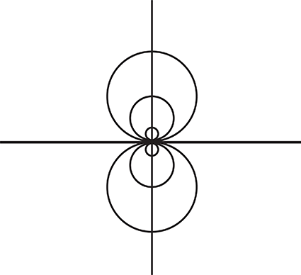
where [latex]{\mu}_{d}{}_{\ }= 2C[/latex] a constant that determines the “strength of the doublet”. This equation can be rearranged:
[latex]{x_1}^2+{\left(x_2+\frac{{\mu }_d}{2\psi }\right)}^2={\left(\frac{{\mu }_d}{2\psi }\right)}^2[/latex]
Noting that for a constant value of [latex]\psi[/latex] the coefficient on the right inside the parenthesis, and the same term added to [latex]{x{}_{2}}[/latex] is a constant resulting in an equation of a circle. The center of the circle changes with changing values of [latex]\psi[/latex] as does the radius of the circle. The result is a series of streamlines for selected values of [latex]\psi[/latex], each of which is a circle centered along the [latex]{x{}_{2}}[/latex] axis as is shown in Fig. 5.4. Notice that the radius of the circle is [latex]\frac{{\mu }_d}{2\psi }[/latex].

Uniform Flow over a Cylinder
The doublet can be added to a uniform flow in the positive [latex]{x{}_{1}}[/latex] direction resulting in a streamfunction given by:
[latex]\psi =Ux_2-\frac{{\mu }_dx_2}{{x_1}^2-a^2+{x_2}^2}\tag{5.22}[/latex]
This equation can be recast in cylindrical coordinates where [latex]{r{}^{2} = x{}_{1}{}^{2}+x{}_{2}{}^{2}}[/latex], [latex]{x{}_{1} = r cos \theta}[/latex] and [latex]{x{}_{2} = r sin \theta}[/latex] and we define [latex]a\ =\ {\left(\frac{{\mu }_d}{U}\right)}^{1/2}[/latex], a constant for a given value of [latex]{U}[/latex], the result is:
[latex]\psi =Ur\ \ sin\theta -Ua^2\frac{sin\ \theta }{r}=Ur\ sin\theta \left(1-\frac{a^2}{r^2}\right)\tag{5.23}[/latex]
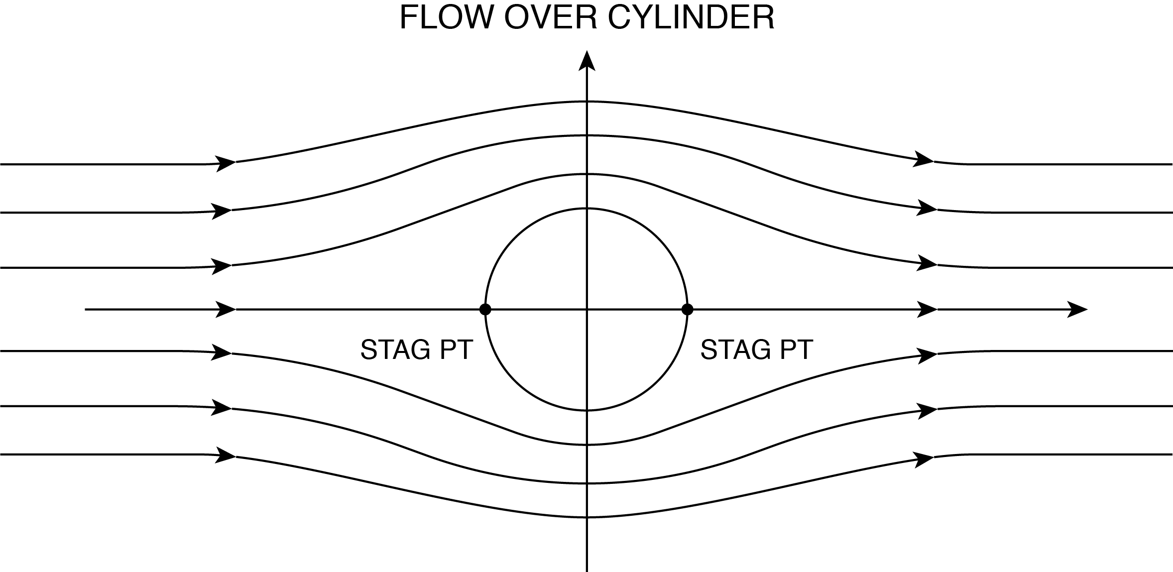
It can be seen that in the limit of large values of [latex]{r}[/latex] the flow reverts back to uniform flow and the contribution for the doublet goes to zero. If we let [latex]\psi =0[/latex] then [latex]{r }= {a}[/latex], a constant. That is to say, the streamfunction of [latex]\psi =0[/latex] is a circle of radius a. So we have now constructed the flow field for uniform flow over a cylinder of radius [latex]{a}.[/latex]
From this the velocity components in the [latex]{r,\theta}[/latex] coordinates are found to be:
[latex]v_r=\frac{\partial \psi }{r\partial \theta }=U\ cos\theta \ \left(1-\frac{a^2}{r^2}\right)[/latex]
[latex]v_{\theta }=-\frac{\partial \psi }{\partial r}=-U\sin\theta \ \left(1+\frac{a^2}{r^2}\right)\tag{5.24}[/latex]
and the velocity vector is [latex]{V{}^{2}}({r,\theta}) = {v_r}^2+{v_{\theta }}^2[/latex]. The streamline distribution is shown in Fig. 5.5. We are only interested in the flow on the outside of the circle, which represents a cylinder. It is important to note that at [latex]{r }= {a}[/latex], the velocity is not zero and depends on [latex]{\theta}[/latex]. So at different positions around the cylinder surface the velocity will change. The largest velocity occurs at [latex]{\theta} = 90{}^{o}[/latex] and [latex]270{}^{o}[/latex], which represents the top and bottom of the cylinder. This is where the streamlines converge the most indicative of high velocity flow. Also at [latex]{\theta} = 0{}^{o}[/latex] and [latex]180{}^{o}[/latex] the velocity is zero. These are stagnation points on the cylinder. Notice also that the streamlines are symmetric about the [latex]{x{}_{1}}[/latex] and [latex]{x{}_{2}}[/latex] axes. This has important implications on the forces that exist on the cylinder caused by the flow.
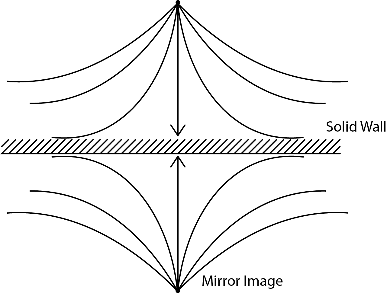
Imaging
There is a method, call imaging, that allows for the insertion of impervious walls or boundaries within a flow. The basic idea here is that a streamline can be used to simulate a solid boundary since it does not allow flow to cross the streamline location. Consequently, if basic flow elements can be combined to yield a streamline that is of the desired shape of a boundary then it satisfies the required flow. For instance, in the condition of uniform flow over a cylinder described above flow elements are combined (uniform flow and a doublet) that result in a simulation of flow over a cylinder, of radius.
Consider the case of a source flow in the vicinity of a flat wall. This may be a simulation of pumping fluid from a well into the surrounding porous region near a solid boundary, such as a rock formation. This could be reversed and have flow into the well (sink). This is shown in Fig. 5.6 where the source is some distance away from the flat wall. We take the wall to be the [latex]x_1[/latex] axis and the source to be a distance “[latex]{l}[/latex]“: away from the wall. If we make the strength of a “mirror image” of the source on the other side of the wall the flow becomes symmetric about the wall with the wall being a streamline (no flow crosses it). Note here that the velocity component in the [latex]{x{}_{2}}[/latex] direction at the wall is zero but not the [latex]{x{}_{1}}[/latex] component. Without providing further details the superposition results in the following equation for the streamfunction:
[latex]\psi =\ {\mu }_s\left({\theta }_1+{\theta }_2\right)[/latex]
[latex]{\theta }_1[/latex] and [latex]{\theta }_2[/latex] are measured from the source and its image, respectively, to any point within the flow. This is similar to what was done when combining a source and sink resulting in the Rankine Oval. In fact the analysis following Eqn. (5.16) can be repeated for this flow but the sign in front of [latex]\theta_2[/latex] replaced with the positive sign shown above for [latex]\psi[/latex].
We introduce one more superposition, that of uniform flow, a doublet and a vortex. The combined streamfunction is:
[latex]\psi =\ Ur\ sin\ \theta \ -{\mu }_d\ \frac{sin\ \theta }{r}-{\mu }_vln\ r\ +C\tag{5.25}[/latex]
where [latex]{C }[/latex] is a constant that can be determined by setting the value of [latex]\psi[/latex] at some point in the flow, as shown below. The coordinate system used here has its origin at the center of the circle generated by the uniform flow and doublet. The added vortex does not add a radial component of velocity, since its flow streamlines are all circles. The result is adding a [latex]{\theta}[/latex] component of velocity throughout the flow that depends on the radial location. In Eqn. (5.25) the direction of the added circumferential flow is clockwise (negative). To summarize the strengths of the elements we have [latex]{U}, {\mu }_d=Ua^2[/latex] and [latex]{\mu }_v=\ \frac{\mathrm{\Gamma }}{2\pi }[/latex]. We can think of these as adjustable parameters to the flow field.
Rewriting Eqn. (5.25) by combining the first and second term as was done for flow over a cylinder and then setting [latex]{r = a}[/latex] , inserting the expression for [latex]{\mu }_d[/latex], as well as setting [latex]\psi =0[/latex], we have:
[latex]C=\mu_vln[/latex] [latex]a[/latex]
This then sets [latex]\psi=0[/latex] on the circle with radius [latex]a[/latex]. Inserting this value of C in Eqn. (5.25) we obtain:
[latex]\psi =\ U\ sin\ \theta \ \left(r-\frac{a^2}{r}\right)-{\mu }_vln\ \frac{r\ }{a}\tag{5.26}[/latex]
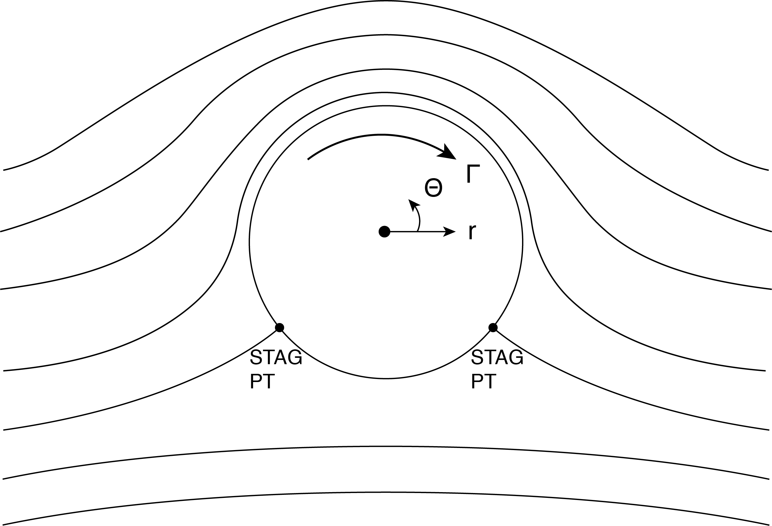
This represents uniform flow over a rotating cylinder as shown in Fig. 5.7, where the streamline representing the cylinder has [latex]{\psi =0}[/latex]. Notice that since we have a clockwise (negative) circulation the cylinder is rotating clockwise. The velocity on the surface of the cylinder now has a contribution caused by the vortex in addition to the velocity found for a non-rotating cylinder. We see that the stagnation points have moved away from along the [latex]x_1[/latex] axis. Since we know that the velocity is zero at the stagnation points we can solve for their location (note that [latex]v_r=0[/latex] everywhere on the cylinder).
[latex]v_{\theta }(r=a)=-\frac{\partial \psi }{\partial r}=-2Usin\ \theta \ +\frac{\mathrm{\Gamma }}{2\pi a}\tag{5.27}[/latex]
or
[latex]sin\theta_{stag}=\frac{\Gamma}{4\pi{aV}}[/latex] for [latex]V_\theta=0[/latex]
We can also determine the pressure distribution around the cylinder surface using Bernoulli’s equation:
[latex]P(r=a)\ =P_{\infty }+\frac{1}{2}\rho U^2-\frac{1}{2}\rho {v_{\theta }}^2-\rho gh\tag{5.28}[/latex]
where [latex]{h }[/latex] is the local height on the circle above the centerline (datum)
[latex]h=a\ sin\ \theta[/latex]
We insert Eqn (5.27) for the velocity on the surface, [latex]v_\theta[/latex], into (5.28) to obtain the expression for the local surface pressure. The integral of the pressure around the circle then determines its net force. First, we find the force component in the [latex]x_2[/latex] direction, this is denoted as the “lift force” per distance into the page, [latex]{F'}_L[/latex]:
[latex]{F'}_L=\ -\oint{P(r=a)\ \ sin\ \theta \ a\ d\theta }[/latex]
Inserting the expression for [latex]{P }[/latex] and noting that integrals of odd powers of the sine functions around the entire circle are zero we are left with:
[latex]{F'}_L=\ -\rho U\mathrm{\Gamma }\ +\ \rho g\pi a^2\tag{5.29}[/latex]
The last term represents the net body force by the fluid on the volume of the circle (per distance into the page) or the buoyancy force. The lift force is usually defined without the buoyancy force included so we write:
[latex]{F'}_L=\ -\rho U\mathrm{\Gamma }\tag{5.30}[/latex]
A few things should be stated about this result. First, recall that the viscous force is not included so this is only due to the pressure distribution. Also, when the circulation is zero there is no lift force (there is still a buoyancy force however). We can conclude that the circulation provides the means to create asymmetric conditions around the circle so that a net pressure force occurs. This expression is often called the Kutta-Joukowsky Law who showed this equation to hold for other shapes as well, and is often used in aerodynamics to determine the lift force on two dimensional airfoils based on the circulation associated with the flow around the wing. The sign convention is such that a counterclockwise rotation results in a downward force, and a clockwise rotation results in a upward force for flow along the positive [latex]{x{}_{1}}[/latex] axis. It is surprisingly accurate for real flows considering the restrictions on its application. This tends to indicate that viscous forces are small at best. It is only accurate for flows that have not separated from the object surface. We will discuss separation when we get into viscous flow affects.
The Kutta-Joukowsky Law (or theorem) as applied to an airfoil requires what is known as the Kutta condition. This is a condition on the flow at the trailing edge that says that the flow exits the airfoil on the top and bottom surfaces of the airfoil with equal velocity and pressure. This implies that the flow does not tend to wrap around the back end or trailing edge of the airfoil and is the boundary condition that allows the calculation of the lift using Eqn. (5.30).
If interested see this website (en.wikipedia.org/wiki/Kutta_condition).
Complex Variables for Potential Flow Analysis
In this section the analysis methods presented for potential flow are expanded using some additional mathematical tools that allows for complex representation of flows and illustrates how complex flows can be analyzed. The flow itself is restricted to the conditions associated with potential flow which allows flows to be evaluated using superposition of the Laplace equation.
Basic Formulation of Complex Variables
For ideal flows we focus on the use of the velocity potential and streamfunction, both of which adhere to the Laplace equation, the former representing the conservation of mass, and the latter indicating irrotational flow. Both can be expressed as:
[latex]\nabla^2f=0[/latex]
where [latex]f[/latex] represents either the velocity potential, [latex]{\phi}[/latex], or the streamfunction, [latex]{\psi}[/latex]. The introduction of either of these variables to define the flow field basically replace the velocity vector as the variable of interest. In arriving at a representation of the flow using complex variable notation the variable [latex]z[/latex] is defined as:
[latex]z=x+iy[/latex]
or in cylindrical coordinates as:
[latex]z=r\ \left(cos\theta+i\ sin\theta\right)=re^{i\theta}[/latex]
Here, [latex]i[/latex] is the traditional representation of [latex]i=\sqrt{−1}[/latex]. Next the Cauchy-Riemann conditions for the two variables and are introduced, which is predicated on the fact that these two variables satisfy the Laplace eqn. and are thus harmonic functions. The Cauchy-Riemann conditions as:
[latex]u=\frac{\partial\phi}{\partial x}=\frac{\partial\psi}{\partial y}[/latex]
[latex]v=\frac{\partial\phi}{\partial y}=−\frac{\partial\psi}{\partial x}[/latex]
It should also be noted that based on this definition the functions [latex]{\phi}[/latex] and [latex]{\psi}[/latex] are orthogonal to each other and it is possible to use one or the other to represent the flow.
A new complex function can be defined, whose real and imaginary parts are based on the velocity potential and streamfunction as:
[latex]F=\phi+i\psi\tag{5.31}[/latex]
The derivative of [latex]F[/latex] in terms of [latex]z[/latex] is defined as:
[latex]W\left(z\right)=\frac{dF}{dz}\tag{5.32}[/latex]
Also:
[latex]\frac{dF}{dz}=\frac{dF}{dz}\frac{\partial z}{\partial x}=\frac{\partial F}{\partial x}[/latex]
Consequently, inserting the definition of [latex]F[/latex] we have
[latex]W\left(z\right)=\frac{\partial\phi}{\partial x}+i\frac{\partial\psi}{\partial x}=u−iv\tag{5.33}[/latex]
This result shows that [latex]W(z)[/latex] represents the “complex velocity” of the flow and is determined by the real velocity components [latex]u,v[/latex].
It is often advantageous to use cylindrical coordinates, expressed as [latex]r,{\theta}[/latex] in two dimensions. The transformation from [latex]x,y[/latex] to [latex]r,{\theta}[/latex] is:
[latex]u=u_rcos\theta−u_\theta sin\theta[/latex]
[latex]v=u_rsin\theta+u_\theta cos\theta[/latex]
The expression for the complex velocity is then (by direct substitution and using the identity of [latex]\cos{\theta}−isin\ \theta=e^{−i\theta}[/latex]) :
[latex]W=\left(u_r−iu_\theta\right)e^{−i\theta}\tag{5.34}[/latex]
The use of the complex variable representation in terms of [latex]F[/latex] can then be converted back into the physical space velocity components, [latex]u,v[/latex], through its derivative relative to the variable [latex]z[/latex]. The magnitude of the local velocity vector is found from [latex]W[/latex] by taking the square root of [latex]WW^*[/latex], where [latex]W^*[/latex] is the complex conjugate of [latex]W[/latex]. Once the velocity is determined then the pressure field is directly determined from the Bernoulli Equation.
Some examples will help illustrate the use of complex variables to represent rather simple flows.
Uniform Flow
A uniform flow of magnitude [latex]U[/latex] in the [latex]x[/latex] direction becomes:
[latex]\phi=Ux=Ur\cos{\theta\ and\ \psi=Uy=Ur\ sin\theta}[/latex]
[latex]F=Ux+iUy=U\left(x+iy\right)=Uz[/latex]
[latex]W=u−iv=\frac{dF}{dz}=U[/latex]
Note that for a flow, [latex]V[/latex], in the [latex]y[/latex] direction [latex]F[/latex] is equal to [latex]-iVz[/latex].
By tilting the uniform flow (direction of [latex]U[/latex]) by angle [latex]{\alpha}[/latex] relative to the [latex]x[/latex] axis the general expression for [latex]F[/latex] in terms of [latex]z[/latex] becomes:
[latex]F=Uze^{−i\alpha}[/latex]
[latex]u=Ucos\ \alpha;v=Usin\ \alpha[/latex]
Source/Sink Flow
A source and sink flow is radial flow from a point and has a strength proportional to its volumetric flow rate such that for any circle centered about the origin of the source or sink, the line integration about the circle yields the volume flow rate per depth into the plane of the circle (recall that we are only dealing with two dimensional flows). A source has a positive strength with flow outward from the center and a sink has a negative strength (flow is inward towards the center). If the volume flow rate per depth is [latex]Q’[/latex] then the strength is designated as [latex]{\mu_s} = Q’/2{\pi}[/latex]. The equations governing the velocity potential lines and streamlines are:
[latex]\phi=\mu_s\ln{r\ and\ \psi=}\mu_s\theta[/latex]
The resulting expression for the complex potential is:
[latex]F=\mu_s\ln{r+i\ \mu_s\ \theta=\ \mu_s(\ln{r+i\ \theta)=\mu_s\ln{\left(re^{i\theta}\right)=\mu_s\ln{z}}}}[/latex]
To locate a source or sink at a point other than the origin, say at location [latex]zo[/latex], we have:
[latex]F=\mu_s\ln(z−z_o)[/latex]
Vortex Flow
A vortex flow is one with only a circumferential velocity component about the origin. The velocity decays proportional to (1/[latex]r[/latex]), where [latex]r[/latex] is the radial coordinate. Notice that the resultant streamlines and potential lines for this flow are orthogonal to the streamlines and potential lines for a source flow. The integral of the velocity around a closed path that includes the origin is defined as the circulation, [latex]{\Gamma}[/latex]. For convenience we chose a circular path of radius [latex]r[/latex]:
[latex]\Gamma=\oint{u\bullet d l=\oint{v_\theta r d\theta=2\pi C}}[/latex]
Where [latex]C=v_\theta r[/latex] which is a constant since [latex]v_\theta[/latex] varies as 1/[latex]r[/latex]. We define [latex]C=\mu_v[/latex] as a measure of the strength of the vortex as
[latex]\mu_v = \Gamma/2\pi[/latex]
So, noting that velocity potential lines are radial and streamlines are circular (counterclockwise) as:
[latex]\phi=\mu_v\theta[/latex]
[latex]\psi={−\mu}_v\ln{r}[/latex]
[latex]F=\mu_v\theta−i{\ \mu}_v\ln{r=\mu_v\left(\theta−i\ ln\ r\right)}[/latex]
[latex]F=\ −i\mu_v\ln{re^{i\theta}}[/latex]
Lastly, the complex velocity can be written as:
[latex]W\left(z\right)=−i\frac{\mu_v}{z}=−i\frac{\mu_v}{r}e^{−i\theta}[/latex]
The negative sign for this expression for [latex]W[/latex] results in a rotation in the counterclockwise direction, which is typically selected as “positive” rotation. Notice the resemblance to the formulation for the source flow and vortex flow representation keeping in mind the orthogonal condition of [latex]\phi[/latex] and [latex]\psi[/latex]. It would be a good exercise to generate plots of the above equations for velocity potential and streamfunction.
There may be some concern that a vortex, which contains vorticity can be considered as irrotational flow. This can be explained as follows. If one were to form a contour anywhere in the flow that does NOT contain the origin (the location of the vortex center) then it can be shown that the circulation is zero. One could conclude that all of the vorticity is located at the center, representing a singularity. The flow driven by this singularity is indeed irrotational. Another way to establish this is to form two contour circles both with centers at the vortex origin but of different radii. It is easily shown then that the difference of the circulation between these two is zero, concluding that for arbitrarily selected contour circles there is no rotational flow between them – so the flow must everywhere be irrotational except at the center.
Flow in a Sector
A sector is defined here to be a region in space near the intersection of two lines, as in a corner with an arbitrary angle. There are general formulations for flows in the region of a sector that can be written in as:
[latex]F=Az^n=Ar^n(\cos{n\theta}+i\sin{n\theta)}\tag{5.35}[/latex]
Where “[latex]n[/latex]” represents a parameter to be specified, usually as a constant for a given flow, and “[latex]A[/latex]” is a constant for a specific flow, and shown below to be proportional to the velocity far from the sector, representative of the flow into the sector. An example of this class of flows is uniform flow where [latex]A=U[/latex] and [latex]n=1[/latex]. Note that uniform flow can be thought of as flow over a flat surface that is parallel to the uniform flow direction (there are no viscous forces so the no slip boundary condition does not hold). The flat surface can be thought of as a sector with an intersection of two lines with the lines being parallel. Or, the angle between the two lines is [latex]\pi[/latex]. The general expression above corresponds to the following expression for velocity potential and streamfunction:
[latex]\phi=Ar^n\cos{(n\theta)}[/latex]
[latex]\psi=Ar^n\sin(n\theta)[/latex]
Using these two expressions we can easily locate lines of constant streamfunction can be found, and in particular when [latex]\psi=0[/latex]: when [latex]\theta=0[/latex] and [latex]\pi/n[/latex]. The flow between these two radial lines represents flow in a “sector”, as seen in the Fig. 5.8, below.
Using the definition of the complex velocity potential, [latex]W[/latex]:
[latex]W=\frac{dF}{dz}=nAz^{n−1}=nAr^{n−1}e^{i(n−1)\theta}[/latex]
Expanding the exponential reveals that the velocity components in [latex]r,\theta[/latex] coordinates are:
[latex]u_r=nAr^{n−1}\cos(n\theta)[/latex]
[latex]u_\theta=nAr^{n−1}\sin(n\theta)[/latex]
By inserting different values for the parameter “[latex]n[/latex]” different flows can be simulated. Some examples are given below.
[latex]n = 1:[/latex]
[latex]u=A[/latex] and [latex]v = 0[/latex] (uniform flow)
[latex]n = 2:[/latex]
[latex]u=2Ar\cos{(\theta)}[/latex]
[latex]v=2Ar\sin{(\theta)}[/latex]
or in Cartesian coordinates: [latex]u=2Ax;\ v=2Ay[/latex]
[latex]\psi=−Ar^2\sin{\left(2\theta\right)}=−Axy[/latex]
or for a constant streamfunction (along a streamline) we have:
[latex]xy = C[/latex]
(where [latex]C[/latex] is a constant determined by the value of [latex]\psi[/latex] at a given location). This latter flow, for a range of values of [latex]C[/latex] yields flow into a right angled corner where the location ([latex]0,0[/latex]) is the position of the corner. Note that [latex]\psi=0[/latex] along the axes. The reader is encouraged to plot this function for different values of streamfunction to visualize the flow.
The corresponding flow into a corner of arbitrary angle, [latex]\alpha[/latex], can be expressed as:
[latex]F=Az^{\pi / \alpha}[/latex]
Note that [latex]Az^n[/latex] is equivalent to [latex]Ar^n [cos(n\theta)+i \enspace sin(n\theta)][/latex] which can then be restated in terms of [latex]\pi / \alpha=n[/latex], so that for [latex]\alpha=\pi /3[/latex] we have [latex]n=3[/latex]. This then relates [latex]n[/latex] to the turning angle of the corner flow. For instance, if [latex]n=3/2[/latex] we have an angle of [latex]2\pi /3[/latex] which is greater than 90o. We can also have flow over a flat plate parallel with the flow if [latex]n=1[/latex].
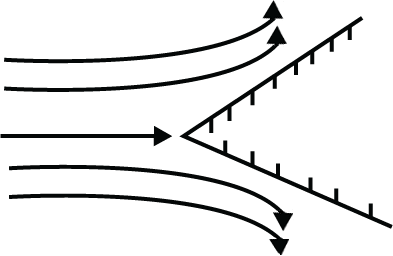
A wedge flow for [latex]\alpha > \pi[/latex]
Wedge flow resembles the flow that divides at the front side (or leading edge) of an object and is a reasonable model for the flow over the leading portion of certain objects. This is illustrated in Fig. 5.9 where flow impinges on an object with a stagnation point at the wedge vertex and then accelerates along the top and bottom surfaces as the streamlines converge. With [latex]\alpha>\pi[/latex] then [latex]n<1[/latex].
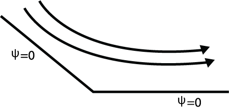
An extreme for wedge flow is flow around a sharp edge, shown in Fig. 5.10 below. Here the flow is moving parallel with a surface, reaches a sharp edge of the surface, and then flows around the edge and then back parallel with the surface. The streamfunction is typically given the value of zero on the surface, and the surface is infinitely thin and flat.
This flow is represented mathematically in terms of a [latex]F(z)[/latex] and constant, [latex]A, n=1/2[/latex] as:
[latex]F\left(z\right)=A\ z^{1/2}[/latex]
[latex]F\left(z\right)=\ A\ r^{1/2}e^{i\frac{\theta}{2}}[/latex]
[latex]\psi=Ar^{1/2}\sin{\frac{\theta}{2}\ }[/latex]
This expression for the streamfunction can be shown to be equal to zero along the surface for [latex]\theta = 0, 2\pi[/latex]. The velocity is obtained from the streamfunction to be:
[latex]u_r=\frac{1}{r}\frac{\partial\psi}{\partial\theta}=\frac{A}{2r^{1/2}}\cos{\frac{\theta}{2}\ \ \ \ \ \ u_\theta=\ −\frac{A}{2r^{1/2}}}\sin{\frac{\theta}{2}}[/latex]
it can be verified that for [latex]0 < \theta < \pi: u_r > 0[/latex] and [latex]u_\theta < 0;[/latex] and [latex]\pi < \theta < 2\pi:u_r < 0[/latex] and [latex]u_\theta > 0[/latex]. This assures the flow reversal around the edge.
Using the flows above written in terms of the constant [latex]A[/latex] we have assumed [latex]A[/latex] to be a real number, but this is not required. We can express this as a complex number by including [latex]e^{−i\beta}[/latex] as a new term: [latex]Ae^{−i\beta}[/latex], where in this expression [latex]A[/latex] is a real number and [latex]{\beta}[/latex] is a constant not the same as used above to define the turning angle of the flow. The result is
[latex]F=Ae^{−i\beta}z^n=Ar^ne^{i(n\theta−\beta)}\tag{5.36}[/latex]
Noting that the real part of F is the velocity potential and the imaginary part is the streamfunction we have:
[latex]\phi=Ar^n\cos(n\theta−\beta)[/latex]
[latex]\psi=Ar^n\sin(n\theta−\beta)[/latex]
This streamfunction expression shows us that when using the complex representation for the constant multiplying [latex]z^n[/latex] there is introduced a rotation of the streamlines through angle [latex]\beta[/latex] using the same coordinate system when compared to the streamfunction when the coefficient is real (not complex).
Doublet
Next, we introduce the concept of a doublet using complex notation (the superposition of a source and sink brought together in the limit as the separation distance goes to zero – but never actually reaches zero separation). This can be expressed as:
[latex]F=\frac{\mu_D}{r}e^{−i\theta}[/latex]
[latex]\phi=\frac{\mu_D}{r}\cos{\theta}[/latex]
[latex]\psi=\frac{\mu_D}{r}\sin{\theta}[/latex]
where [latex]\mu_D[/latex] is a constant representing the strength of the doublet. Lines of constant streamfunction [latex]\psi = B[/latex] become:
[latex]\psi=B=\frac{−\mu_D\ r\ sin\theta}{r^2}=\frac{−\mu_Dy}{\left(x^2+y^2\right)}[/latex]
[latex]x^2+(y+\frac{\mu_D}{2B})^2=\left(\frac{\mu_D}{2B}\right)^2[/latex]
This last equation illustrates that we have an equation of a circle with the center located along the [latex]y[/latex] axis with the position changing depending on the value of [latex]B[/latex], which implies different streamfunction values and therefor different streamlines for each [latex]B[/latex]. The radius of each circle is determined by ([latex]\mu_D/2B[/latex]) which depends on the value of the streamfunction. Also, each circle is tangent to the [latex]x[/latex] axis at [latex]x = 0[/latex], or the line with [latex]\theta = 0[/latex] at [latex]r = 0[/latex]. See the sketch below in Fig. 5.11 of streamlines.
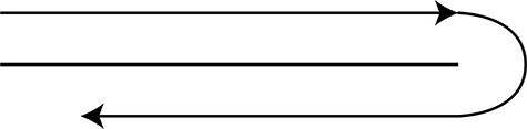
Rankine Half-Body
More complicated flows using complex variable representation based on the superposition of simpler flows can be formed with any proper representation of the simpler flows. An example is the Rankine half-body. In some ways this has characteristics similar to the wedge flow identified above in that we are interested in the flow approaching an object and the initial region near the leading edge. However, rather than flat plates forming a corning with a sharp point we have the simulation of flow over a rounded leading-edge surface. In this case we superimpose a uniform flow with a source located at the origin of the coordinate system, both expressed using complex variables. Here we have:
[latex]F=Uz+\mu_s\ln{z}[/latex]
To obtain the velocity components in the ([latex]r,\theta[/latex]) coordinates we use the definitions of the velocity potential (or we could use the streamfunction):
[latex]u_r=\frac{\partial\phi}{\partial r}=Ucos\ \theta+\frac{\mu_s}{r}[/latex]
[latex]u_\theta=\frac{1}{r}\frac{\partial\phi}{\partial\theta}=−Usin\ \theta[/latex]
At the very front, or leading edge of the body, the velocity should become zero, representative of a stagnation point. So, setting each velocity component equal to zero we can determine where the stagnation point should occur.
[latex]u_r=0:\ \ Ucos\ \theta=−\frac{\mu_s}{r}[/latex]
[latex]u_\theta=0:\ \ U\sin{\theta=0}[/latex]
There are two solutions to the above set of equations: [latex]\theta = 0[/latex] and [latex]\theta = \pi[/latex]. However, for [latex]\theta = 0[/latex] the value of [latex]r[/latex] becomes negative from the first equation, which is an invalid condition so the only realistic solution for the location of the stagnation point is ([latex]\mu_s /U,\pi[/latex]). By increasing the source strength, [latex]\mu_sv[/latex], the stagnation point moves further upstream in the flow. The streamfunction that passes through this point is found by noting that [latex]u_\theta=−\frac{\partial\psi}{\partial r}[/latex] such that integrating and setting [latex]\theta = \pi[/latex] then [latex]\psi_{stag}=\mu_s\pi[/latex]. Since the streamfunction passing through the stagnation point is on the body then a general streamfunction expression for the body becomes
[latex]\psi_{body}=Ur_{body}\sin{\theta_{body}}+\mu_s\theta_{body}[/latex]
In this expression the subscript “body” represents [latex]r,\theta[/latex] coordinates that are on the body which will be a constant value of the streamfunction. A plot of a constant value of [latex]\psi_{body}=\mu_s\pi[/latex] (which is specified by the stagnation point given above) can be used to determine the body surface. In general, we have:
[latex]r_{body}=\frac{\mu_s(\pi−\theta_{body})}{U\sin{\theta_{body}}}[/latex]
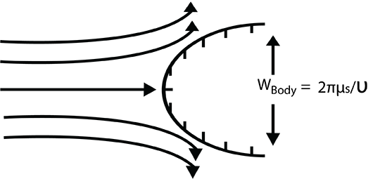
One can imagine that for increasing r in the first or fourth quadrant the influence of the source will diminish (since we are moving away from the source). Consequently, the flow is expected to eventually become streamlines that are again parallel with the oncoming flow. For the streamline of the body, in the limit of large r we can write an expression for the total width of the body, [latex]w_{body}[/latex] :
[latex]w_{body}=\frac{2\pi\mu_s}{U}[/latex]
By increasing the source strength for a given freestream velocity [latex]U[/latex] the width of the body increases and it is possible to model flow over the object of any desired width.
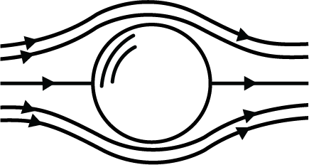
Enclosed Bodies
It is possible to continue on with the idea of flow over an object and create a completely enclosed object (this requires an enclosing streamline such as a circle or ellipse) to simulate flow over the enclosed object. The streamlines inside the body are of no interest here, just those flowing around the outside of the body and how the velocity and pressure vary. As an example, we simulate the flow over a circular cylinder. This will involve the superposition of a uniform flow and a doublet at the origin. This can be expressed in our complex representation as:
[latex]F\left(z\right)=Uz+\frac{\mu_D}{z}[/latex]
The strength of the doublet for a given flow [latex]U[/latex] will determine the radius of the cylinder. Consider a desired radius [latex]a[/latex] for a given uniform flow [latex]U[/latex]. We can write the complex potential for the circle as:
[latex]F\left(z\right)=Uae^{i\theta}+\frac{\mu_D}{ae^{i\theta}}[/latex]
Noting that the streamfunction is the imaginary part of this expression which yields:
[latex]\psi=\left(Ua−\frac{\mu_D}{a}\right)\sin{\theta}[/latex]
We can force the value of the streamfunction to be [latex]\psi=0[/latex] at [latex]r = a[/latex] by setting the strength of the doublet to [latex]\mu_D=Ua^2[/latex]. Consequently, we end up with flow of velocity [latex]U[/latex] over a cylinder of radius [latex]a[/latex]. We insert the strength of the doublet into the expression for [latex]F(z)[/latex]:
[latex]F=U(z+\frac{a^2}{z})[/latex]
Again, we are only interested in the flow outside of the cylinder, as shown in Fig. 5.13.
As we will see later, it is possible, through a proper transformation of the flow over a cylinder, to obtain the flow over objects, such as an airfoil. However, to make this more physically correct we will want to introduce circulation to the flow to simulate the circulation that occurs for an actual airfoil that provides the lift force experienced by the airfoil. Recall from a vortex flow that circulation is based on circumferential flow, with strength proportional to the [latex]u_\theta[/latex] velocity component. Superimposing a uniform flow over a cylinder with radius [latex]a[/latex], with a vortex of strength [latex]\mu_v[/latex] rotating in the clockwise direction, results in the following:
[latex]F=U\left(z+\frac{a^2}{z}\right)+i\mu_v\ln{z+c}[/latex]
where we add the constant [latex]c[/latex], this will allow us to assign the value of the streamfunction to the cylinder surface, at [latex]r = a[/latex]. By setting [latex]z=ae^{i\theta}[/latex] to be on the cylinder surface the value of the complex potential can be evaluated and thereby obtaining the streamfunction value in terms of the unknown constant [latex]c[/latex]. By setting [latex]c=\ −i\mu_v\ln{a}[/latex] it is straightforward to show that the streamfunction is in fact equal to zero for all [latex]\theta[/latex] at [latex]r = a[/latex]. Then using this value for [latex]c[/latex] and combining c with the second term (combining the [latex]ln[/latex] terms) results in the following expression for the flow over a cylinder with circulation:
[latex]F=U\left(z+\frac{a^2}{z}\right)+i\mu_v\ln{\frac{z}{a}}[/latex]
Note that the above expression is for circulation with clockwise rotation, for counterclockwise rotation the ln term is negative.
The velocity field associated with the above expression for [latex]F(z)[/latex] is:
[latex]u_r=U\left(1−\frac{a^2}{r^2}\right)\cos{\theta}[/latex]
[latex]u_\theta=-U\left(1+\frac{a^2}{r^2}\right)\sin{\theta−\frac{\mu_v}{r}}[/latex]
Notice that it is the vorticity that provides the circumferential flow component. Also, along the surface of the cylinder the velocity is not necessarily zero. In fact, since this is a streamline then the value of [latex]u_r[/latex] must be zero so no flow crosses the cylinder, but [latex]u_\theta[/latex] is only zero at two points. These points are stagnation points because both velocity components are zero resulting in zero velocity. The locations of these two points are found by setting [latex]u_\theta = 0[/latex] and solving for [latex]\theta[/latex]:
[latex]\sin{\theta_{stagnation}=\frac{\mu_v}{2Ua}}=\frac{\Gamma}{4\pi Ua}[/latex]
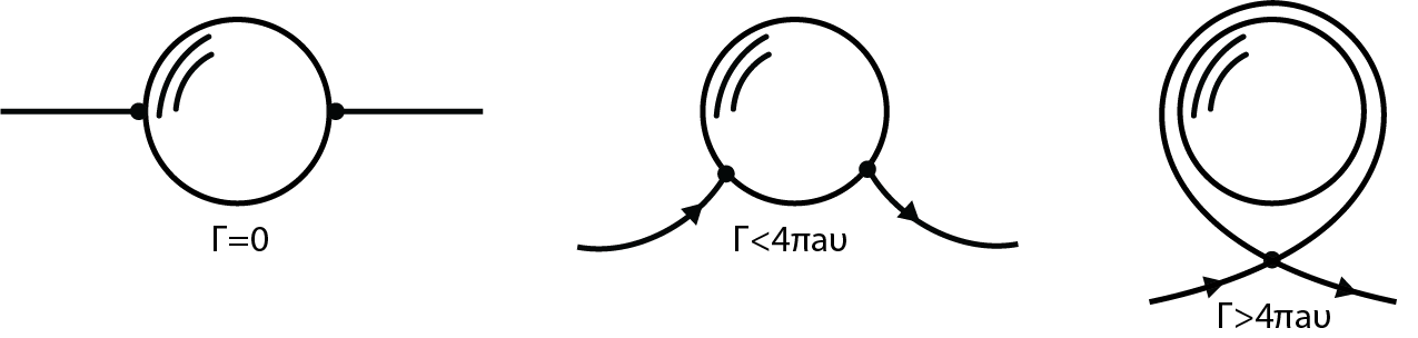
If the circulation is zero ([latex]\mu_v = 0[/latex]) then the stagnation points are at [latex]\theta = 0, 2\pi[/latex], implying symmetric flow both relative to the [latex]x[/latex] and [latex]y[/latex] axis. See Fig. 5.14 for representation of stagnation points for different circulation conditions. For clockwise rotation greater than zero stagnation points will move to the third and fourth quadrants. For counterclockwise rotation, the stagnation points will be in the first and second quadrants. When the strength of the clockwise circulation is large enough to result in [latex]\theta = 3\pi /2[/latex] and the two points coincide on the “bottom” of the cylinder. For larger circulation strengths than this the stagnation point actually moves off of the cylinder.
At this point it is instructive to evaluate the consequences of the added circulation to flow over a cylinder. As we have seen from above, the circulation removes symmetry across the [latex]x[/latex] axis within the flow. That is the streamline distribution for the third and fourth quadrants is different from the first and second quadrants of the flow. However, this circulation does not change the symmetry that exists across the [latex]y[/latex] axis (the flow in the first and fourth quadrants is symmetric with the second and third quadrants). Recall from the Bernoulli equation (viscous forces are ignored and we have a steady flow) that the pressure field will retain a similar symmetry with the velocity field. The symmetry across the [latex]y[/latex] axis indicates the pressure on the “front” half of the cylinder will be identical to that on the “back” half of the cylinder and the net force in the x direction will be zero. However, across the [latex]x[/latex] axis the loss in velocity symmetry implies a difference in pressure distribution on “top” of the cylinder versus the “bottom”. Also, for circulation with a clockwise rotation the velocity on top will be greater than that on the bottom resulting in lower pressure on the top. The net effect is an upward force on the cylinder by the pressure field. If the rotation is reversed there would be a net downward force on the cylinder.
The determination of the force on a body with external flow around it in potential flow can be determined from the Kutta-Joukowski law which relates the net lift on the body to the circulation, [latex]\Gamma[/latex], generated by the flow and the magnitude of the freestream velocity, [latex]U[/latex], as:
[latex]Lift/span=−\rho U\Gamma[/latex]
This relationship is shown in an earlier part of this chapter. It is also shown below in the context of conformal mapping. In this formulation, if the circulation is negative (clockwise) then the force direction will be positive (upward lift) when there is positive flow over the body (left to right). This can be derived for any shaped two-dimensional body with an associated circulation calculated from the line integral about an enclosed area that includes the body. This law can be shown through the use of Newton’s law relating total force (lift plus pressure) to rate change of momentum and the integration of the pressure field obtained from the Bernoulli equation for steady two-dimensional, irrotational inviscid flow. We show this also in the next section. The interested student can review the derivation of this from many references or online (en.wikipedia.org/wiki/Kutta–Joukowski_theorem) using the basic tools of complex representation of the velocity field.
For the circular cylinder case the circulation is specified within the strength of the vortex and is used in conjunction with the freestream velocity to specify the flow conditions associated with a given freestream velocity and cylinder radius.
Conformal Transformations
As mentioned previously it is possible to transform the results for flow over a cylinder with circulation to that of flow over an airfoil, allowing the determination of the lift force through the solution to the magnitude of the lift force for flow over the cylinder. The idea of a transformation in this sense is that by altering the coordinate system it is possible to change from a circular geometry to a different geometry. Once this transformation is specified it is possible to calculate the flow at certain points within the circular geometry and assign the flow results to points in the new, different geometry.
Consider a mapping function [latex]\zeta=\zeta(z)[/latex] which establishes a relationship between coordinates [latex]\zeta[/latex] and [latex]z[/latex] (where again [latex]z = x +iy[/latex]). Consequently, a known solution expressed in [latex]\zeta[/latex] can then be transformed into the [latex]z[/latex] coordinate. The condition for conformal mapping in this sense is that the velocity potential (which satisfied the Laplace equation in the original coordinate must also be satisfied in the new coordinate. The other condition is that new coordinate must satisfy the Cauchy-Riemann equations. These state the following where the new coordinates are, say, ([latex]\xi,\eta[/latex]) and the original coordinates are ([latex]x,y[/latex]):
[latex]\frac{\partial\xi}{\partial x}=\frac{\partial\eta}{\partial y}\ and\ \frac{\partial\xi}{\partial y}=−\frac{\partial\eta}{\partial x}[/latex]
Under these conditions it can be shown that the complex potential, [latex]F(z)[/latex], in a given coordinate which determines the velocity potential and streamfunction, can be shown to satisfy the Laplace equations for the velocity potential and streamfunction in the [latex]\zeta[/latex] plane. The local solutions in the [latex]z[/latex] plane are found from the solutions in the [latex]\zeta[/latex] plane by using the relationship given by [latex]\zeta=\zeta(z)[/latex]. In other words, a solution at a point in [latex]\zeta[/latex] has the same value at the corresponding point in [latex]z[/latex]. In additional to this, if we take our previous definitions for [latex]W(z)[/latex] we can write:
[latex]W\left(z\right)=\frac{dF(z)}{dz}=\frac{d\zeta}{dz}\frac{dF(\zeta)}{d\zeta}=\frac{d\zeta}{dz}W(\zeta)[/latex]
This says that the mapping function derivative with respect to [latex]z[/latex] defines the relationship between the complex velocity solutions in each coordinate frame. Lastly, it can also be shown that the strengths of the various flow elements used within one frame are not altered in the transformed coordinate frame. These relationships now allow one to solve a given problem, such as flow over a cylinder with circulation, and interpret the results in another coordinate frame which may change the geometry of the object.
As an example, consider using the Joukowski transformation:
[latex]z=\zeta+\frac{C^2}{\zeta}[/latex]
with [latex]C[/latex] being a constant that determines the shape of the boundary in transformation. For instance a circle of radius a given by [latex]\zeta=ae^{i\theta^\ast}[/latex] while setting [latex]C = a[/latex] results in:
[latex]z=a\left(e^{i\theta^\ast}+e^{−i\theta^\ast}\right)=2a\cos{\theta^\ast}[/latex]
and the resultant [latex]z[/latex] plane shape will be a flat plate extending from [latex]-2a[/latex] to [latex]+2a[/latex] along the [latex]x[/latex] axis in the [latex]z[/latex] plane. Note that here, [latex]\theta*[/latex] is used to represent the angle coordinate in the [latex]\zeta[/latex] plane (not [latex]z[/latex] plane). This illustrates a transformation between a circle, in [latex]\zeta[/latex], to a flat plate in [latex]z[/latex]. Here we are interested in points outside of the radius of the circle and how they transform to points in the [latex]z[/latex] plane.
Continuing this, by noting that the stagnation points in the [latex]\zeta[/latex] plane are determined by the circulation, as shown previously for flow over a cylinder, then when the circulation is zero the stagnation points are at [latex]\theta\ast= 0,\pi[/latex]. The stagnation points in the z plane then are found through the transformations as at [latex]x=\pm2a[/latex], or at the ends of the flat plate.
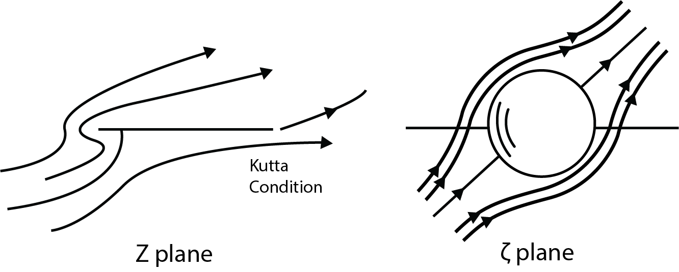
The more interesting case is when we have a flat plate with the freestream flow at some angle, [latex]a[/latex], to the [latex]x[/latex] axis. This is usually defined to be the angle of attack. When this occurs a stagnation point will form on the “bottom” side of the plate when the freestream velocity has a positive angle relative to the x axis (which forms the freestream velocity direction). This is shown in fig. 5.15, below. At this stagnation point the flow separates, with part of the flow moving forward in the positive [latex]x[/latex] direction and some of the flow moves in the negative [latex]x[/latex] direction. The latter flow then must turn around the corner or edge of the flat plate as shown in the figure. Also, the trailing edge will have a relative movement of the stagnation point away from the trailing edge of the plate, resulting in flow having to go around the trailing edge and up along the surface. Since this flow is inviscid the potential flow velocity around an infinitely thin plate must go to infinity since the radius of curvature is zero. This does not happen in a real flow due to viscous effects slows the fluid and resulting in a finite radius of curvature and flow separation at the edge. In a real airfoil the leading edge has a finite thickness and can potentially eliminate flow separation unless the angle of attack is too large. But the trailing edge is typically very thin. The resulting flow condition preventing separation at the trailing edge is the Kutta condition imposed at the trailing edge. See the earlier discussion of the Kutta condition. The idea is that the flow adjusts itself to prevent this separation by imposing local circulation near the trailing edge to offset the separation flow. If circulation is added to the flow to move the stagnation point to the trailing-edge then the flow at the trailing edge will have equal velocity on the top and bottom surfaces of the plate (and by Bernoulli equation equal pressures) such that the flow will leave the trailing edge smoothly and not wrap around the trailing edge.

Considering flow around a cylinder in the [latex]\zeta[/latex] plane at an angle of attack of [latex]\alpha[/latex] relative to the [latex]x[/latex] axis, or [latex]\theta =0[/latex]. The uniform freestream must be rotated by angle [latex]\alpha[/latex], and this results in the following representation of the complex potential:
[latex]F\left(\zeta\right)=U\left(\zeta e^{−i\alpha}+\frac{a^2}{\zeta e^{−i\alpha}}\right)+i\mu_v\ ln\frac{\zeta}{a}[/latex]
However, we wish to impose the Kutta condition as well. To do this we must add circulation equivalent to moving the stagnation point to the trailing edge, or [latex]z = 2a[/latex]. For this value of [latex]z[/latex] the corresponding value of [latex]\zeta[/latex] is [latex]a[/latex], which is on the cylinder at ([latex]a,0[/latex]). To achieve this additional rotation of the flow by angle [latex]\alpha[/latex] in the [latex]\zeta[/latex] plane is required. We use the equation for the stagnation point position, [latex]\theta_stag[/latex], to see that the required circulation is [latex]\Gamma=4\pi Uasin\ \alpha[/latex].
So inserting this value of circulation into the vortex strength above we obtain:
[latex]F\left(\zeta\right)=U\left(\zeta e^{−i\alpha}+\frac{a^2}{\zeta e^{−i\alpha}}\right)+i2Ua\ sin\alpha\ ln\frac{\zeta}{a}[/latex]
This can be written in terms of the [latex]z[/latex] plane with [latex]\zeta=\frac{z}{2}+\sqrt{\left(\frac{z}{2}\right)^2−a^2\ }[/latex]
as:
[latex]F(z)=U\left(\left(\frac{z}{2}+\sqrt{\left(\frac{z}{2}\right)^2−a^2}\right)e^{i\alpha}+\frac{a^2e^{i\alpha}}{\left(\frac{z}{2}+\sqrt{\left(\frac{z}{2}\right)^2−a^2}\right)}+i2a\ sin\alpha\ ln\left(\frac{1}{a}\left(\frac{z}{2}+\sqrt{\left(\frac{z}{2}\right)^2−a^2}\right)\right)\right)[/latex]
Noting that the imaginary part of [latex]F(z)[/latex] represents the streamfunction. Fig. 5.16 below represents the flow in both the [latex]z[/latex] and [latex]\zeta[/latex] planes.
We can easily determine the lift force with the known circulation to be:
[latex]L=\rho U\Gamma=4\pi\rho U^2a\sin{\alpha}[/latex]
Expressing this nondimensionally, as a lift coefficient by dividing by ([latex]1/2 \rho U^2 c[/latex]) where [latex]c[/latex] is the length of the plate (the chord length) which is equal to [latex]4a[/latex] we obtain:
[latex]C_L=2\pi\sin{\alpha}[/latex]
This is the theoretical lift coefficient for a thin (flat) airfoil at an angle of attack of [latex]\alpha[/latex], as was shown previously in this chapter. For small angles of attack, we have [latex]C_L=2 \pi \alpha[/latex].
Blasius Theorem and Lift Force for an Arbitrary Body
The lift force for a rotating cylinder in a uniform inviscid flow is given by [latex]L = - \rho U \Gamma[/latex] (where the circulation is positive if counterclockwise and flow is from left to right). What is rather amazing is that the object shape is not critical in the use of this same equation as long as the value of the generated circulation is determined properly.
The Blasius Theorem (also referred to as the Blasius Integral Laws), is a means to obtain the total force on the object within a flow. Ideally the surface velocity distribution would be found, then using the Bernoulli equation the pressure along the surface is found, which could be integrated to find the net force on the object. However, this procedure can be circumvented through the use of the Blasius Theorem.
At any location on the object surface the expression for the local force, [latex]dF[/latex], in terms of the velocity potential, can be found. Specifically, the force is decomposed into drag and lift components, noting that drag is in the negative [latex]x[/latex] direction, as:
[latex]dF=dF_D−idF_L=−Pdy−iPdx=−iP(dx−idy)[/latex]
Now to extend this around the entire object it is needed to integrate around the closed path forming the object (by sign convention we go counterclockwise) as:
[latex]F_D−iF_L=−i\oint{Pdz^\ast}[/latex]
[latex]z^\ast=x−iy[/latex]
Where [latex]z*[/latex] is the complex conjugate of [latex]z[/latex]. The pressure is determined from the Bernoulli equation with the surface velocity written as
[latex]{U_s}^2=\left[(u+iv)(u−iv)\right]_s[/latex]
[latex]u+iv=({u_r}^2+{u_\theta}^2)^{1/2}e^{i\theta}[/latex]
[latex]dz=|dz|e^{i\theta}[/latex]
The last two expressions show that the velocity and surface are parallel with each other, both at the same angle, as must be the case for a solid surface in inviscid flow. So, we can show that [latex](u+iv)dz*[/latex] is a real number (using the fact that the velocity slope equals the surface slope, or [latex]v/u = y/x[/latex], so the imaginary part goes to zero) and that [latex](u+iv)dz*=(u-iv)dz[/latex]. Finally, the velocity is determined by:
[latex]W=\left(u−iv\right)[/latex]
So, by inserting for the pressure in terms of the velocity from the Bernoulli equation, and using the above express for [latex]U_s[/latex] along with the relationship for [latex]W[/latex] in terms of the velocity components it can be show after a bit of manipulation that:
[latex]F_x−iF_y=\frac{i\rho}{2}\oint{W^2dz}[/latex]
The above expression is valid for steady, potential flow and often called the “Blasius Theorem”. Notice that the drag component is the negative of the real part of the right hand side and the lift component is the negative of the imaginary part.
In potential flow the integration around any closed contour (say a contour around the surface of a body versus a contour around the body far from the body itself) can be shown to be the same. For this to be true there can be no singularities that occur between the contours. So, in this case no sources or sinks or vortices, etc. can exist between the surface contour and a contour far from the surface. Flow around an arbitrarily shaped object may be generated by putting a distribution of singularities, such as vortices, around the shape contour and adjust their strength distribution to form a closed contour of some desired shape. This is discussed in detail in the next chapter. In the flows considered here there are no singularities outside of the body itself. So, we can take a contour far from the body out into the free stream. All of the distributed singularities will appear, from far away, as if they are all located at the coordinate system origin (assumed to be located near or in the object-although this may not be necessary). The superposition representation of the complex potential can be written by eliminating the small distances from singularity location and the origin. One can then insert the complex velocity associated with the superposition into the above equation for force. The unique aspect here is that as the contour moves further and further away from the body the complex velocity can be simplified by dropping terms that are small, such as for a vortex we have terms like [latex]i\Gamma /2 \pi z[/latex] and for a doublet we have [latex]\mu_D /z^2[/latex]. Note that here a positive circulation is designated as clockwise, as is typically done in aerodynamic applications. If we only retain terms ~[latex]1/z[/latex] and perform a series expansion then by complex variable theory the contour integral is equal to [latex]2 \pi i \sum{residuals}[/latex].
The residuals are determined by taking the square of the complex velocity as shown in the integral above, and dropping terms higher than say [latex]1/z[/latex]. Then the residual is the coefficient of the [latex]1/z[/latex] term which is multiplied by [latex]2 \pi i[/latex] to obtain the value of the integral. The real part is [latex]F_D[/latex] and the negative of the imaginary part is [latex]F_L[/latex].
This can be illustrated using the complex potential for a uniform flow, vortex and doublet (flow over a rotating cylinder): [latex]F=Uz+\mu_v\ln{z+\frac{\mu_D}{z}}[/latex]. Taking the [latex]z[/latex] derivative to form the complex velocity, [latex]W[/latex], and then squaring this and only retaining up to the [latex]1/z[/latex] terms, the coefficient of the [latex]1/z[/latex] term will be [latex]2i \mu_v[/latex] resulting in the following for the force:
[latex]F_D−iF_L=\frac{i\rho}{2}\left(2\pi i\frac{\left(i\Gamma U\right)}{\pi}\right)=0−i\left(\rho U\Gamma\right)[/latex]
This states the there is a net lift force dependent of the circulation and zero drag force and is the identical to the result presented previously. The circulation here is that due to the sum total effect of the distribution of vortices around the object. This result is often called the Kutta-Zhukhovsky theorem.
