VIII. Boundary Layer Flows
In this chapter, we discuss the physical attributes associated with boundary layer flows. The governing equations are developed from the Navier-Stokes equation. The laminar boundary layer flow characteristics and interpretation of the associated forces generated by the flow are presented and discussed. This flow is a viscous dominated flow, rather than a pressure dominated flow. We will not explore the details associated with boundary layers on curved surfaces or surfaces that have flows influenced by an existing pressure gradient. Some physical insight into these conditions will be presented, however, and the concept of flow separation is introduced.
The pioneering work of Ludwig Prandtl soon after the beginning of the 20th century lays most of the groundwork for boundary layer analysis. His work has lead to an entire field of study that allows a combination of viscous dominated flows with inviscid flows. Prandtl used a very detailed combination of experimental and analytical methods to approach a very complex problem — the influence of fluid friction on streamline flows. He was very interested in wing theory and how to model real wing flows and their associated forces of lift and drag. The concept of a thin airfoil theory was developed and applied to three-dimensional wings. Here we will look at the basic physics associated with boundary layer theory and how these flows can be modeled for the laminar flow conditions. Turbulent flows are introduced in a later chapter.
Physical Attributes of a Boundary Layer
A boundary layer flow is defined to be the region of a larger flow field that is next to the surface and has significant effects of wall frictional forces. Since the region of interest is near the surface and the surface is assumed to be impervious to the flow then the velocity is nearly parallel to the surface. The general flow is shown in Fig. 8.1. Flow is from left to right and there is an upstream “leading edge” where the surface begins. At the leading edge (defined as the coordinate system origin), the flow immediately next to the surface begins to experience frictional forces due to the no slip boundary condition.
The fluid outside of this thin layer is directly unaffected by the wall friction. As the flow goes downstream the slower moving fluid near the surface exerts frictional forces on the fluid further away from the surface. This process is one of diffusion of momentum loss in a direction normal to the surface that results in a reduction of the local fluid velocity. The rate of diffusion depends on the viscosity of the fluid. As this happens the region slowed by friction grows such that the thickness of the boundary layer, [latex]\delta[/latex], increases along the flow direction. At the outer edge of this viscous region, where the flow is no longer affected or slowed by the surface generated friction, the velocity is called the “freestream” value. The boundary layer flow shown in Fig. 8.1 represents a laminar flow condition where the boundary layer thickness extends further away from the surface at locations further along the flow direction. Turbulent flow has a similar trend but has some distinct differences in the velocity distribution and is discussed in a later chapter. Both laminar and turbulent flows must follow the no-slip boundary condition at the surface, resulting in zero relative velocity at the surface. The boundary layer thickness is affected by the turbulence and results in a thicker boundary layer in general.
Although we said that the flow is principally along the surface in the narrow boundary layer, there needs to also be a “wall-normal” velocity component, or [latex]u{}_{2}[/latex] using our coordinate system. The requirement of a non-zero velocity component away from the surface can be shown by using a control volume starting from the leading edge and extending downstream an arbitrary distance [latex]{x}_{1}[/latex] as shown in Fig. 8.2. Note that the control volume has the same area for flow inlet and outlet in the stream-wise direction, that is [latex]\mathrm{h}[/latex] is a constant. By applying conservation of mass to this control volume we obtain the following for steady flow:
[latex]0={\dot{m}}_3+{\dot{m}}_2-{\dot{m}}_1[/latex]
where the subscripts refer to the different mass flows shown in Fig. 8.2, subscript 1 is the flow coming into the control volume from the left at the leading edge, subscript 2 is the flow going out the right side at distance x downstream and subscript 3 is flow that goes out the top. The flow coming in at the leading edge has a uniform velocity of U over the vertical distance h. The outflow at distance [latex]x{}_{1}[/latex] has been slowed by friction such that the velocity varies from zero at the surface to U at the outer edge of the boundary layer. Integrating this downstream velocity profile over the same vertical distance h will result in a lower mass flow rate than at the leading edge since [latex]{\dot{m}}_2<{\dot{m}}_1[/latex]. Consequently, [latex]{\dot{m}}_3[/latex] > [latex]0[/latex] or, there must be a positive outflow, [latex]{\dot{m}}_3[/latex], resulting in a velocity component out the top of the control volume. The no-slip boundary condition requires that all velocity components are zero at the surface. This implies that the vertical velocity component must start at zero and increase with increasing [latex]x{}_{2}[/latex]. Also, streamlines associated with the flow must deflect upwards along the flow direction to account for the nonzero [latex]{x}_{2}[/latex] velocity component, as is shown in Fig 8.2.
The characteristics of the developing velocity profile along the flow direction, [latex]{x}_{1}[/latex], can be used to understand the distribution of the surface shear stress [latex]\tau_{s}[/latex]. Since the boundary layer grows larger in the flow direction, as more and more of the fluid above the surface is slowed by friction, then at any given height, [latex]{x}_{2}[/latex], the velocity in the [latex]{x}_{1}[/latex] direction must decrease going in the [latex]{x}_{1}[/latex] direction. That is [latex]\frac{\partial u_1}{\partial x_1} < 0[/latex].
The result of this is that the velocity distribution has a decreasing value of [latex]\frac{\partial u_1}{\partial x_2}[/latex] near the surface. That is to say, the velocity is always zero at the surface and always extends to [latex]\mathrm{U}[/latex] at the edge of the boundary layer, [latex]{x}_{2} = \delta[/latex], so as [latex]\delta[/latex] increases the velocity derivatives [latex]\frac{\partial{u_1}}{\partial{x_2}}[/latex] everywhere within the flow must decrease. Based on this, the value of [latex]\frac{\partial u_1}{\partial x_2}[/latex] at the surface decreases in the [latex]{x}_{1}[/latex] direction. Using the definition of the shear stress and noting that [latex]\frac{\partial u_1}{\partial x_1}=0[/latex] at the surface, we see that
[latex]{\tau }_s=\mu \ {\left(\frac{\partial u_2}{\partial x_2}\right)}_{x_2=0}\tag{8.1}[/latex]
where the subscript [latex]x_2=0[/latex] means that it is evaluated at the surface. Since the surface velocity derivative decreases along [latex]{x}_{1}[/latex] then so does the surface shear stress and the qualitative result is the trend of [latex]\tau_s[/latex] shown in Fig. 8.2. Notice that the surface shear stress does not reach a constant value, as in pipe flow, since the flow never becomes fully developed, or [latex]\frac{\partial{u_1}}{\partial{x_1}}\neq 0[/latex].
If the surface is perfectly flat then the freestream flow outside the boundary layer will be nearly parallel with the surface (in the [latex]{x}_{1}[/latex] direction) at velocity U, except for the small upward velocity component described earlier. For parallel straight flow the change of pressure along the flow, and normal to the flow, is zero as we saw in inviscid flow. If we anticipate that the thickness, [latex]\delta[/latex], of the boundary layer is relatively thin (we will show this to be the case later in this chapter when we develop the boundary layer equations) then the change of pressure due to hydrostatic effects between the outer edge of the boundary layer and the surface is small, even if the fluid is a liquid. However, even if hydrostatic pressure rise is not small across the boundary layer the change in pressure along the flow should in fact approach zero near the surface because the change in pressure along the flow is zero just outside of the boundary layer. This is explained by the following. The hydrostatic pressure change is the same between two vertical points evaluated at different locations along [latex]{x}_{1}[/latex]. So the difference of pressure in the [latex]{x}_{1}[/latex] direction, [latex]\frac{\partial P}{\partial x_1}[/latex] will be identical for positions near the edge of the boundary layer and near the surface. So if [latex]\frac{\partial P}{\partial x_1\ }=0[/latex] just outside the boundary layer then it is also zero inside the boundary layer. The net effect of this is that for a flat surface the pressure gradient along the flow is essentially zero. We will show this to be true based on the governing equations later in this chapter. We could extend this further for a curved surface and deduce that the pressure gradient for flow over the curved surface is the same outside and inside the boundary layer if the boundary layer is thin.
So a summary of the main attributes we will rely on for the analysis of boundary layers at this point are: (i) the boundary layer is thin, [latex]\delta[/latex] >> [latex]L[/latex], (ii), the wall normal velocity is small but finite, [latex]{u}_{2}[/latex] << [latex]{u}_{1}[/latex], (iii) for a (nearly) flat surface the pressure gradient is zero, [latex]{\partial {P}}/{\partial {x}_{1}} = 0[/latex], (iv) the outer edge of the boundary layer velocity is the freestream velocity, U, which is determined by inviscid flow conditions.
Boundary Layer Equations
The boundary layer equations are a somewhat simplified form of the Navier-Stokes equations based on the physical attributes of the flow, listed above. The flow here is taken to be steady and two-dimensional, with velocity components in [latex]{x}_{1}[/latex] and [latex]{x}_{2}[/latex], which we designated by ([latex]{u}_{1}, {u}_{2}[/latex]). Note that it is possible to have a more complex unsteady three dimensional version of boundary layer flow that is beyond the scope here. As part of the solution we will show that [latex]{u}_{1}[/latex] >> [latex]{u}_{2}[/latex]. We assume the surface is perfectly flat and parallel to the oncoming fluid flow direction so there is no pressure gradient along the flow direction. Finally, we neglect any gravitational forces and assume we have incompressible flow. Strictly speaking the boundary layer equations do not require the pressure gradient to be zero, and can be treated as a parameter that allowed for some curvature of the surface (not flat).'
With the above conditions we write the [latex]{x}_{1}[/latex] direction Navier-Stokes equation as:
[latex]\rho \left(u_1\frac{\partial u_1}{\partial x_1}+u_2\frac{\partial u_1}{\partial x_2}\right)=\mu \left(\frac{{\partial }^2u_1}{\partial {x_1}^2}+\frac{{\partial }^2u_1}{\partial {x_2}^2}\right)\tag{8.2}[/latex]
we combine this with the differential conservation of mass for an incompressible flow:
[latex]\left(\frac{\partial u_1}{\partial x_1}+\frac{\partial u_2}{\partial x_2}\right)=0\tag{8.3}[/latex]
At this point we have two-dimensional partial differential equations in two variables. It is worth noting here that the pressure gradient in the y direction, across the flow, is reduced to a very small number under the conditions that the [latex]u{}_{2}[/latex] component of velocity is very small compared with [latex]u{}_{1}[/latex], and that the boundary layer is thin so that there is essentially zero hydrostatic pressure variation across the flow. This can be shown by noting that all terms in the [latex]{x}_{2}[/latex] momentum equation containing [latex]u{}_{2}[/latex] become very small and the body force term is small since changes in [latex]{x}_{2}[/latex] are small, therefor the pressure gradient in [latex]{x}_{2}[/latex] must also be small. This process will become clearer in our discussions of scaling of the [latex]{x}_{1}[/latex] momentum equation below.
Next we scale the variables in the governing equation. This means coming up with appropriate scaling for each variable (dependent and independent) that is on the order of the maximum value of the variable. For instance, the characteristic length scale for flow over a flat plate with length L would be just L. Similarly, the characteristic velocity scale for the [latex]{x}_{1}[/latex] velocity component would be the freestream velocity, U. Below is listed the characteristic scales for the various variables (note that the scales may not be constant values as is noted by the choice of scale for [latex]{x}_{2}[/latex]):
[latex]x_1-L\tag{8.4}[/latex]
[latex]x_2-\ \delta[/latex]
[latex]u_1-U_{\infty }[/latex]
[latex]u_2-unknown[/latex]
In general L can be any length of surface. We select [latex]\delta[/latex] to be the boundary layer thickness that coincides with this selected length in the analysis below. That is to say that the largest value of [latex]\delta[/latex] occurs at [latex]x_1=L[/latex]. But in general [latex]\delta[/latex] varies as we move in the [latex]{x}_{1}[/latex] direction. We do not know how large [latex]u{}_{2}[/latex] may be, but we can determine this by examining the conservation of mass, Eqn. (8.3). To do this we use the above scaling to form nondimensional variables, denoted by the superscript ``*'' by dividing each variable by its scale value:
[latex]{x_1}^*=\frac{x_1}{L}\tag{8.5}[/latex]
[latex]{x_2}^*=\frac{x_2}{\delta }[/latex]
[latex]{u_1}^*=\frac{u_1}{U}[/latex]
[latex]{u_2}^*=\frac{u_2}{V_s}[/latex]
where [latex]V{}_{s}[/latex] is an unknown scale for variable [latex]u{}_{2}[/latex] and is to be determined. Inserting these non-dimensional variables into Equation (8.3), where [latex]u=u^*U[/latex], etc., we obtain:
[latex]\frac{U{}}{L}\left(\frac{\partial {u_1}^*}{\partial {x_1}^*}\right)+\frac{V_s}{\delta }\left(\frac{\partial {u_2}^*}{\partial {x_2}^*}\right)=0=\frac{\partial {u_1}^*}{\partial {x_1}^*}+\frac{V_sL}{\delta U}\left(\frac{\partial {u_2}^*}{\partial {x_2}^*}\right)\tag{8.6}[/latex]
where the last set of terms is a consequence of dividing the first set of terms through by [latex]\frac{U}{L}[/latex]. The coefficient of the first term become one, the coefficient multiplying the second term becomes [latex]\frac{V_sL}{\delta U}[/latex]. At this point we apply an order of magnitude analysis of the terms. Both terms have to balance each other in the equation, being of opposite sign. We use the nomenclature [latex]\mathcal{O}(1)[/latex] to indicate that the value of a term is ``order one''. By proper scaling of the variables we assume that, [latex]\frac{\partial {u_1}^*}{\partial {x_1}^*}[/latex], is [latex]\mathcal{O}(1)[/latex]. That is to say, by proper scaling this derivative using scales that are approximately the maximum value of the variable then the resultant term will not be a very large or a very small number, but rather ``order one''. We make the same assumption for the derivative [latex]\frac{\partial {u_2}^*}{\partial {x_2}^*}[/latex]. Consequently since neither of these derivatives are zero, as we have noted previously for the boundary layer, then for this equation to be valid we must have
[latex]\frac{V_sL}{\delta U}=\ \mathcal{O}(1)[/latex]
With this we can assign the value of the [latex]u{}_{2}[/latex] velocity scale to be:
[latex]V_s=U\frac{\delta }{L}\tag{8.7}[/latex]
By doing so then each term is [latex]\mathcal{O}(1)[/latex]. Keep in mind that we are not trying to find exact values but at this point trying to determine approximately how large or small the scaling values should be. If we now take Equation (8.7) and insert this into Equation (8.6) we end up with:
[latex]\left(\frac{\partial u^*}{\partial x^*}\right)+\left(\frac{\partial v^*}{\partial y^*}\right)=0\tag{8.8}[/latex]
for the nondimensional representation of the conservation of mass with the scaling of the variables given by the relationships above.
Using our new found scaling for [latex]u{}_{2}[/latex] we continue this same non-dimensional process for the other terms in the Navier-Stokes Equation (8.2). That is, replacing all of the variables with the nondimensional variables, and then dividing the resulting equation by the coefficient of the first term, [latex]\frac{{\rho U}^2}{L}[/latex] resulting in:
[latex]{u_1}^*\frac{\partial {u_1}^*}{\partial {x_1}^*}+{u_2}^*\frac{\partial {u_1}^*}{\partial {x_2}^*}=\frac{\mu }{\rho UL}\left(\frac{{\partial }^2{u_1}^*}{\partial {{x_1}^*}^2}+\frac{L^2}{{\delta }^2}\frac{{\partial }^2{u_1}^*}{\partial {{x_2}^*}^2}\right)\tag{8.9}[/latex]
This nondimensional equation, that incorporates the scaling given above, leads to some profound conclusions. First note that the coefficient on the right hand side of the two terms in parentheses, which are the fluid friction terms, is the inverse of the Reynolds number that we define for boundary layer flows: [latex]Re_L=\frac{{\rho U}_{\infty }L}{\mu }[/latex]. This Reynolds number is based on the freestream velocity and the total length of the surface. We have included a subscript L on the Reynolds number to inform us of the selected length scale. Next we have the coefficient [latex]\frac{L^2}{{\delta }^2}[/latex] of the last term in parentheses. Since we have assumed that the boundary layer is thin ([latex]\delta \ll L[/latex]) then this coefficient will be large. Since each of the derivatives is assumed to be order one through proper scaling, then the entire second term in parentheses must be much larger than the first term, or:
[latex]\frac{{\partial }^2{u_1}^*}{\partial {{x_1}^*}^2} \ll \frac{L^2}{{\delta }^2}\frac{{\partial }^2{u_1}^*}{\partial {{x_2}^*}^2}\tag{8.10}[/latex]
So the frictional forces in the boundary layer are dominated by the term containing [latex]\frac{{\partial }^2{u_1}^*}{\partial {{x_2}^*}^2}[/latex]. This term is the net angular deformation caused by shearing stress. The first term is the linear deformation caused by the normal viscous stress. This result is consistent with the fact that the thin boundary layer will have very large derivatives of velocity in the [latex]{x}_{2}[/latex] direction when compared with the [latex]{x}_{1}[/latex] direction. So neglecting the normal viscous stress contribution the resulting nondimensional form of the boundary layer equation for steady flow over a flat surface is:
[latex]{u_1}^*\frac{\partial {u_1}^*}{\partial {x_1}^*}+{u_2}^*\frac{\partial {u_1}^*}{\partial {x_2}^*}=\frac{\mu }{\rho UL}\left(\frac{L^2}{{\delta }^2}\frac{{\partial }^2{u_1}^*}{\partial {{x_2}^*}^2}\right)\tag{8.11}[/latex]
There is one more conclusion that can be arrived at from this scaling. Noting that the shearing contribution derivative, [latex]\frac{{\partial }^2{u_1}^*}{\partial {{x_2}^*}^2},[/latex] is [latex]\mathcal{O}(1)[/latex] as are each of the nondimensional acceleration terms on the left hand side, then in order for this equation to be balance [latex]\left(\frac{\mu }{\rho UL}\frac{L^2}{{\delta }^2}\right)[/latex] should also be [latex]\mathcal{O}\left(1\right)[/latex]:
[latex]\frac{\mu }{\rho UL}\left(\frac{L^2}{{\delta }^2}\right)\sim \ \mathcal{O}(1)[/latex]
or
[latex]Re{_L}\sim \frac{L^2}{{\delta }^2}\tag{8.12}[/latex]
This last condition implies that for a thin boundary layer to exist the Reynolds number should be large. So for large Reynolds numbers in boundary layer flows with a surface length of L the boundary layer thickness, [latex]\delta[/latex], is proportional to the square root of [latex]Re{}_{L}[/latex] which we can write as:
[latex]\frac{\delta }{L}={\frac{C}{\sqrt{Re}_{x_1}}}\tag{8.13}[/latex]
where C is some unknown constant inserted to make the equation quantitatively correct. Consequently, for very small values of [latex]L[/latex] the boundary layer conditions do not hold since [latex]Re{}_{L}[/latex] is small.
The nature of the governing equation given by Eqn. (8.11) is that it is a parabolic partial differential equation. Since it only requires one boundary condition in [latex]{x}_{1}[/latex], which can be selected at [latex]{x}_{1} = 0[/latex] (the leading edge) where the velocity is given as [latex]U[/latex], then the solution is independent of any downstream boundary condition. This means it can be solved at any arbitrary position [latex]{x}_{1}{}_{\ }[/latex] along the surface. This also implies that the result (8.13) is valid by replacing L with location [latex]{x}_{1}{}_{.\ \ }[/latex]. Doing this we have a Reynolds number based on any position [latex]{x}_{1}[/latex]:
[latex]Re_{x_1}=\frac{\rho Ux_1}{\mu }[/latex]
and Equation (8.13) can be expressed as:
[latex]\frac{\delta }{x_1}={\frac{C}{\sqrt{Re}_{x_1}}}\tag{8.14}[/latex]
Equation (8.14) predicts that the boundary layer grows proportional to the distance [latex]x{}_{1}{}^{1/2}[/latex] (recall that there is a factor [latex]x{}_{1}[/latex] contained in the [latex]{Re}_{x_1}[/latex]); also this will not be valid for very small values of [latex]x_1[/latex].
Using Eqn. (8.12) the final form of the boundary layer equation for flow over a flat surface is:
[latex]{u_1}^*\frac{\partial {u_1}^*}{\partial {x_1}^*}+{u_2}^*\frac{\partial {u_1}^*}{\partial {x_2}^*}=\frac{{\partial }^2{u_1}^*}{\partial {{x_2}^*}^2}\tag{8.15}[/latex]
From our discussion of the characteristics of the boundary layer we have the following boundary conditions:
(i) [latex]{x}_{2}= 0: u{}_{1}=0, u{}_{2} =0[/latex] (no-slip),
(ii) [latex]{x}_{2} = \delta: u{}_{1}[/latex] = U
(iii) [latex]{x}_{1} = 0: u{}_{1}[/latex] = U
This equation seems to have eliminated all parameters (like viscosity, density and Re). However, recall that [latex]{x}_{2}[/latex] is non-dimensionalized using [latex]\delta[/latex] and also [latex]u_2[/latex] is non-dimensionalized using [latex]\delta[/latex]. In order to determine [latex]\delta[/latex] one needs to know the relationship between [latex]\delta[/latex] and Re. So even though we may be able to solve Eqn. (8.15) there is still work to do to interpret the results.
Laminar Boundary Layer Solution
The solution to the boundary layer equations for steady flow over a flat surface parallel with the oncoming flow, with the associated boundary conditions, is called the Blasius solution. This was accomplished around 1913 originally by Paul Blasius, a graduate student of Prandtl's. Noting that Eqn. (8.15) shows that the basic equation consists of two convective acceleration terms and one viscous term which can be written in terms of the original dimensional variables as:
[latex]\rho \left(u_1\frac{\partial u_1}{\partial x_1}+u_2\frac{\partial u_1}{\partial x_2}\right)=\mu \left(\frac{{\partial }^2u_1}{\partial x_2}\right)\tag{8.16}[/latex]
with the conservation of mass as Equation (8.3).
Following the general solution approach of Blasius we can introduce the streamfunction, and use it to replace the velocity components:
[latex]u=\frac{\partial \psi }{\partial x_2};\ \ \ \ v=-\frac{\partial \psi}{\partial x_1}\tag{8.17}[/latex]
We have previously shown that this definition for two dimensional, incompressible flow satisfies conservation of mass, by inserting these expressions into Equation (8.3). Substituting these two expressions in terms of [latex]\psi[/latex] for the two velocity components in Equation (8.16) results in:
[latex]\frac{\partial \psi }{\partial x_2}\left(\frac{{\partial }^2\psi }{\partial x_1\partial x_2}\right)-\frac{\partial \psi }{\partial x_1}\left(\frac{{\partial }^2\psi }{\partial x^2_2}\right)=\nu \left ( \frac{\partial^3\psi}{\partial x^3_2} \right )\tag{8.18}[/latex]
Here we have also divided through by density to obtain the kinematic viscosity, [latex]\nu = \mu / \rho[/latex], as the coefficient of the viscous term which is the only parameter in the equation (a constant for a given fluid). Although the resulting equation seems formidable the use of the streamfunction has reduced the two velocities into a single dependent variable [latex]\psi[/latex].
The streamfunction, with SI units of [latex]m{}^{2}[/latex]/s, is nondimensionalized as:
[latex]f\left(\eta \right)=\frac{\psi }{{\left(\nu x_1U\right)}^\frac{1}{2}}\tag{8.19}[/latex]
a non-dimensional similarity variable, [latex]\eta[/latex], is defined to combine [latex]x_{1}[/latex] and [latex]x[/latex] into a variable:
[latex]\eta =\frac{x_2}{{\left(\frac{\nu x_1}{U}\right)}^{1/2}}=x_2{\left(\frac{U}{\nu x_1}\right)}^{1/2}\tag{8.20}[/latex]
The new variable f is assumed to be only a function of [latex]\eta[/latex]. This will be verified by inserting these new variables into the original equation and see if the result is only [latex]\eta[/latex] dependent. Each of the terms in Eqn. (8.18) are transformed into the ([latex]f,\eta[/latex]) variables using the chain rule similar to what was done in chapter 7 to determine the governing equation for a suddenly accelerated flat surface. Similarly, the non-dimensional stream function of Eqn. (8.18) can be written in terms of [latex]u_1[/latex] and [latex]u_2[/latex] and inserted into Eqn. (8.16). The result is the following, using the prime designation to represent the derivative with respect to [latex]\eta[/latex]
[latex]u_1=\frac{\partial\psi}{\partial x_2}\frac{\partial \psi }{\partial \eta }\frac{\partial \eta }{\partial x_2}=\frac{\partial \psi }{\partial \eta }\left(\frac{U}{\nu x_1}\right)=f'U\tag{8.21}[/latex]
[latex]u_2=\frac{U}{2\sqrt{Re_x}}\left( \eta f' -f \right)\tag{8.22}[/latex]
[latex]\frac{\partial u_1}{\partial x_1} =\frac{\eta}{2}\frac{U}{x_1}f^{"}\tag{8.23}[/latex]
[latex]\frac{\partial u_1}{\partial x_2}=Uf^{"}\left(\frac{U}{\nu x_1}\right)^{1/2}\tag{8.24}[/latex]
[latex]\frac{{\partial }^2u_1} {\partial {x_2}^2} = \frac{U^2f^{'''}}{\nu x_1} \tag{8.25}[/latex]
Substituting all of this into our boundary layer equation, (8.16), with a little bit of manipulation the result becomes:
[latex]f^{'''}+\frac{1}{2}ff^{''}=0\tag{8.26}[/latex]
This now is a single variable ordinary differential equation, which shows that [latex]f = f(\eta)[/latex] resulting in a similarity equation. To obtain a solution the boundary conditions need to be specified in terms of [latex]\eta[/latex]. Specifically there are three: [latex]x_2=0:u_1=u_2=0[/latex] (no slip condition) so
[latex]f\left(0\right)=f'\left(0\right)=0[/latex]
[latex]x_2\ge \delta :u_1=U[/latex] so
[latex]f'\left(\eta \to \infty \right)=1.0\tag{8.27}[/latex]
The no slip condition for [latex]u_{2}[/latex] results in [latex]f\left(0\right)=0[/latex] since [latex]f'\left(0\right)=0[/latex] for the no slip condition of [latex]u_{1}[/latex] so by Eqn. (8.22) [latex]f\left(0\right)=0[/latex]. Also, we take the boundary condition at the edge of the boundary as [latex]\delta \rightarrow \infty[/latex] since [latex]U[/latex] remains constant for [latex]x_2[/latex] > [latex]\delta[/latex] . Physically this imposes an asymptotic limit of the solution for large [latex]\delta[/latex], or beyond the edge of the boundary layer.
The solution to Equation (8.26) along with the boundary conditions of Equations (8.27) is rather straight forward using a Runge-Kutta technique. However, this was not the case when Blasius solved this equation numerical by hand back in the early 1900s at the University of Göttingen.
The results of the numerical solution of Eqn (8.26) are expressed as [latex]f'\left(\eta \right)=u_1/U_{\infty }[/latex] and are shown in Figure (8.3). Obviously [latex]u_{1}/U[/latex] varies from zero at the surface ([latex]\eta = 0[/latex]) and approaches 1.0 at [latex]x_{2} = \delta[/latex]. The value of [latex]\delta[/latex] can be determined from this plot, however one must select a value of [latex]f'\left(\delta \right)[/latex] close to 1.0, and typically 0.99 is chosen. At this value of [latex]f'\left(\delta \right)[/latex] the value of [latex]\eta \simeq 5.0[/latex]. Using the definition of [latex]\eta[/latex] given above and setting it equal to 5.0 when [latex]x_{2} = \delta[/latex] results in:
[latex]5=\frac{\delta }{{\left(\frac{\nu x_1}{U}\right)}^{1/2}}[/latex]
Rearranging this yields an expression for the boundary layer versus [latex]x_{1}[/latex]:
[latex]\frac{\delta }{x_1}=\frac{5}{{Re_{x_1}}^{1/2}}\tag{8.28}[/latex]
This shows that [latex]C = 5[/latex] in Eqn. (8.13). Eqn. (8.28) allows for the evaluation of the boundary layer thickness, [latex]\delta[/latex], at any [latex]x_{1}[/latex] location for a given value of U and viscosity [latex]\nu[/latex]. Using the solution in Fig. (8.3) also allows for the evaluation of the velocity components, [latex]{u}_{1}[/latex] and [latex]{u}_{2}[/latex] and any location [latex]x_{1}[/latex] and [latex]x_{2}[/latex] in the boundary layer.
Other aspects of the flow can also be found from the solution. The total force on the surface caused by fluid flow friction can be found from the surface stress, [latex]{\tau }_s=\mu \frac{\partial u_1}{\partial y}[/latex], which requires evaluating the velocity derivative at the surface, [latex]x_{2}[/latex] = 0. The non-dimensional form is used to evaluate [latex]\frac{\partial u_1}{\partial y} \text{ at } x_2 =0[/latex]. Using Eqn. (8.24) we have:
[latex]{\left(\frac{\partial u_1}{\partial x_2}\right)}_{x_2=0}=f''(0)U^{3/2}\sqrt{\frac{\rho }{\mu x_1}} \tag{8.29}[/latex]
where [latex]f''(0)[/latex] is the second derivative of f evaluated at [latex]\eta =0[/latex]. From the Blasius solution [latex]f^{''}\left(0\right)=0.332[/latex]. After multiplying Equation (8.29) by the dynamic viscosity to obtain the surface stress and then dividing by [latex]\frac{1}{2}\rho {U}^2[/latex] which defines the surface skin friction coefficient, [latex]c_f,[/latex] the result is:
[latex]c_f=\frac{{\tau }_s}{\frac{1}{2}\rho U^2}=\ \frac{0.664}{{Re_{x_1}}^{1/2}}\tag{8.30}[/latex]
The above expression can be used to find the local surface stress at any [latex]x_1[/latex] location along the surface (recall [latex]Re_{x_1}=\frac{\rho U_{\infty }x_1}{\mu }[/latex]). This then indicates that for a given freestream velocity of a given fluid the surface shear stress decreases as [latex]{x_1}^{-1/2}[/latex]. The final step to determine the total drag force, [latex]F{}_{D}[/latex], on the surface is to integrate [latex]\tau_s[/latex] over the entire surface using the results of Equation (8.30). [latex]F_d = \int_{0}^{L}\tau_s dx_1S[/latex] which is written as the drag coefficient, [latex]{C}_{D}[/latex]:
[latex]C_D=\frac{F_D}{\frac{1}{2}\rho {U^2{(LS)}}}=\frac{1.328}{{Re_L}^{1/2}} \tag{8.31}[/latex]
where [latex]S[/latex] is the span of the surface in the [latex]x_3[/latex] direction.
The drag coefficient provides a nondimensional convenient expression to determine the overall drag force on a surface. Knowing the length of plate, L, one calculates the [latex]Re{}_{L}[/latex] and then uses (8.31) to find [latex]F_D[/latex].
Pressure Gradient Effects
The above discussion is concerned with forces caused by fluid friction for flow over a surface. The other major contribution to the total force acting on a surface when there is flow over the surface is that of pressure. When the pressure is uniform within the flow it has no contribution to the change of momentum of the flow (zero pressure gradient) along the flow. However, as we have seen for inviscid flow, a pressure distribution over a surface results in a force and this pressure distribution is significantly altered by the flow conditions. Consider flow over a cylinder or Rankine oval where the velocity variation results in a pressure variation at the surface of the oval. The force for inviscid flow can be obtained from the Bernoulli equation to evaluate the local pressure which is then integrated over the surface.
For viscous flows the pressure and surface frictional forces both need to be integrated over the surface. However, importantly, these two can not be treated as independent of each other. That is to say, the pressure distribution is influenced by the velocity distribution, or vice versa, as we see from the Navier-Stokes equation which contains a pressure gradient term. Consequently, one can expect that the velocity distribution within the boundary layer will be altered as the pressure gradient changes (in other words we no longer have Eqn. (8.3) which assumes [latex]\frac{\partial P}{\partial x_1}=0[/latex]). With an altered velocity profile the velocity gradient at the surface also changes indicating that the surface stress changes. The link between pressure gradient and surface stress can be very complex, influenced by the conditions that result in a specific pressure gradient. This is made apparent by considering the Navier-Stokes equation evaluated at the surface, with no slip boundary conditions. In this case acceleration terms are all zero and there is a balance of pressure and viscous forces at the surface:
[latex]\frac{\partial P'}{\partial x_1}=\mu {\left(\frac{{\partial }^2u_1}{\partial {x_2}^2}\right)}_{x_2=0}={\left(\frac{\partial \tau }{\partial x_2}\right)}_{x_2=0} \tag{8.32}[/latex]
For the boundary layer, assuming it is thin, the pressure gradient can be evaluated outside the boundary layer as discussed previously. Also, in this expression we have absorbed the body force term into the pressure term: [latex]P'=P+\rho gh[/latex] where h is the height above some datum. This form of the pressure plus body force accounts for the hydrostatic pressure variation that may occur along the direction [latex]x_1[/latex] caused by changes in elevation given by changes in h.
Eqn. (8.32) provides insight into the flow conditions very close to the surface for changing pressure gradients. For instance, if [latex]\frac{\partial P'}{\partial x_1} < 0[/latex] (a ``favorable pressure gradient'') then the pressure decreases in the flow (or [latex]x_{1}[/latex]) direction. This implies from Eqn (8.32) that the surface stress decreases moving away from the surface as one might expect since it ultimately reaches zero at the edge of the boundary layer, for inviscid flow conditions. For conditions of very large favorable pressure gradients ([latex]\frac{\partial P'}{\partial x_1} \ll 0[/latex]) the decrease of stress with [latex]x_{2}[/latex] is greater and the boundary layer becomes thinner, and the wall shear stress becomes larger. The distribution of stress is shown in qualitatively Fig. 8.4.
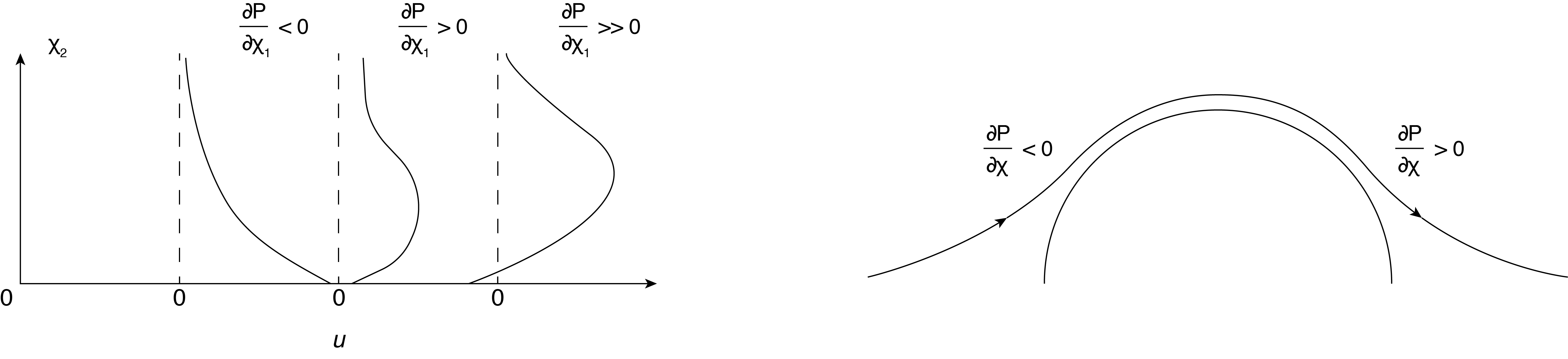
If the pressure gradient has a positive sign, [latex]\frac{\partial P'}{\partial x_{1}}[/latex] > [latex]0[/latex], (an "adverse pressure gradient'') the stress increases with increasing [latex]x_{2}[/latex] away from the surface again as shown in Eqn. (8.32). This implies that at some point the stress reaches a maximum, and then decays to zero at the edge of the boundary layer. See Fig. 8.4. As the adverse pressure gradient increases one can suspect that the gradient of stress near the surface also becomes larger, forcing the stress to approach zero or even go negative as shown in Fig. 8.4. Under these conditions, of negative stress, the implications are that the sign reversal causes the flow in a region near the wall to actually go in the negative, or upstream, [latex]x_{1}[/latex] direction. This is the definition of ``flow separation''. Separated flow no longer adheres to boundary layer flow as part of the flow near the surface is moving upstream and part of the flow further from the surface is moving downstream. This generally results in swirling flow near the surface.
What can cause such a large adverse pressure gradient? One common situation is the existence of large surface curvature, such as flow over a cylinder of diameter D and length S into the page, shown in Fig. 8.5. In these cases the [latex]{x}_{1}[/latex] coordinate is taken as curving along the surface in the flow direction. On the upstream side of the cylinder the pressure gradient is negative as the flow accelerates with increasing velocity. The growth of [latex]\delta[/latex] is not as large as for the zero pressure gradient case, as noted above. As the flow continues over the top (or bottom) of the cylinder the pressure gradient becomes positive, increasing pressure in the flow direction. This is caused by the decrease of velocity for the flow beyond the top (bottom) of the cylinder. The inviscid flow over a cylinder has been studied previously (as a superposition of uniform flow and doublet). For this inviscid case the pressure can be found from the Bernoulli equation and the result can be expressed as the pressure coefficient as:
[latex]c_p=\frac{P-P_{\infty }}{\frac{1}{2}\rho U^2}=1-\frac{{v_s}^2}{U^2}=1-4sin^2\theta\tag{8.33}[/latex]
where [latex]P_{\infty }[/latex] is the pressure for upstream (or downstream) of the cylinder and [latex]v_s[/latex] is the surface velocity at any point around the cylinder (zero at the front and back stagnation points and maximum at the top and bottom). A plot of this inviscid pressure distribution around the cylinder is shown in Fig. 8.5. Notice that the pressure distribution is symmetric and the net force caused by pressure is zero. The maximum pressure is at the stagnation points, as expected, and equal to [latex]P_\infty + \frac{1}{2}pU^2[/latex] from Bernoulli equation.
With the addition of viscous effects, for flow over a cylinder, as described above, the adverse pressure gradient on the rear portion of the cylinder results in flow separation when the freestream flow is sufficiently large. The flow then forms a ``wake'' across the back of the cylinder consisting of swirling, turbulent flow. The result is an asymmetric flow pattern around the cylinder and an asymmetric pressure distribution. In the wake the pressure is not as high as in the inviscid case. We see in the pressure coefficient plot that for viscous flows the pressure recovery on the downstream side is not as large as the inviscid case and the net affect is a downstream drag force. Turbulent flows tend to have a greater pressure recovery and a lower nondimensional drag coefficient ([latex]C_D=\frac{F_D}{\frac{1}{2}\rho U^2DS}[/latex]) when compared with laminar flow.