Chapter 9: Gene Regulation
Genes can be regulated in several different ways, and be regulated transcriptionally (at the gene-level), post-transcriptionally (at the mRNA level), translationally, and post-translationally. Splicing of mRNA can also be regulated and there are many other inputs to regulation still.
Clearly, transcriptional regulation and post-transcriptional regulation are best suited for study by nucleic acid sequence bioinformatics because techniques such as ChIP-seq and RNA-seq can be used to measure the inputs and outputs of these modes of regulation. Here we will focus on regulation by transcription factors using ChIP-seq and regulation by microRNAs using small RNA-seq and RNA-seq.
9.1 Transcription Factors and ChIP-seq
Transcription factors (TFs) are proteins that bind to DNA and are capable of regulating the transcription of genes. TFs can be activators, which activate transcription of the genes they regulate, or repressors, which block the transcription of the genes they regulate.
9.1.1 ChIP-seq Peak identification
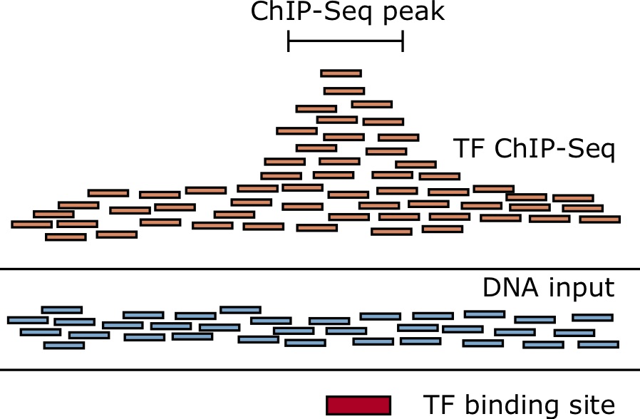
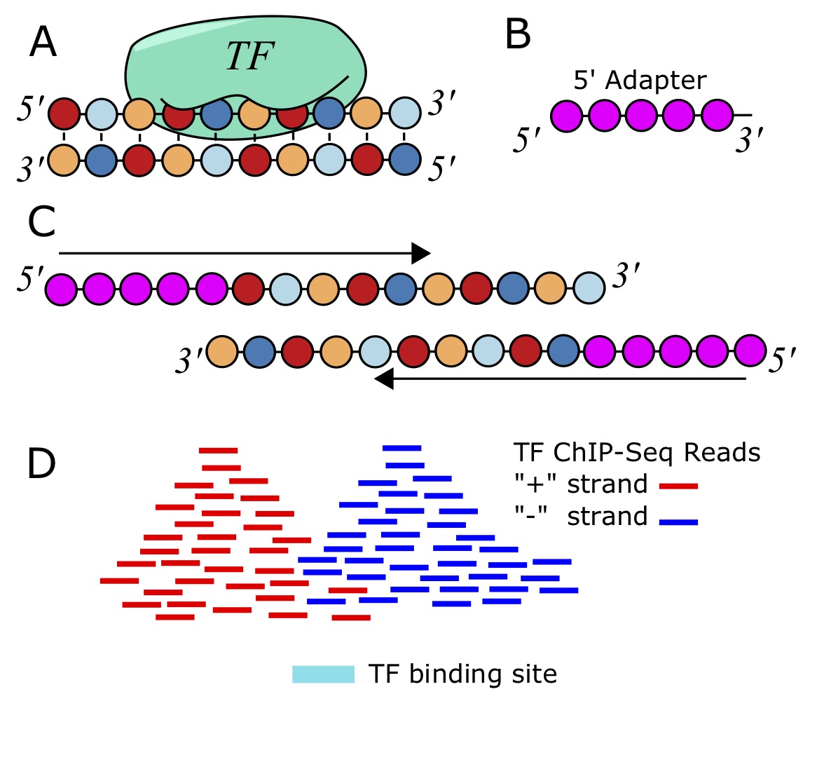
ChIP-seq measures the genome-wide binding of a TF by sequencing DNA fragments that are bound to the TF in a controlled experiment [92 - 94]. Antibodies that recognize epitopes in the protein of interest are used to "pull-down" the protein. When cross-linking is used, such as by adding formaldehyde, everything sticks together, holding the protein to the DNA that it is bound to. After the antibodies and associated chromatin are precipitated out from the solution and isolated, they can be reverse-crosslinked, and then a DNA-extraction is performed. The fragments of DNA are then sequenced using deep sequencing. Despite best efforts to just isolate fragments directly bound the the TF of interest, a lot of spurious reads make it through the process as well. Therefore, we need to sequence a control sample without the antibody, either using the immunogloblulin (IgG) or just naked DNA (input), so that we can look for statistical enrichment of the reads that align to a particular genomic location from the ChIP-Sample compared to this control sample.
Short read alignment with [latex]\texttt{bowtie}[/latex]
Once we have the the reads from the high-throughput sequencer, typically in a FASTQ file, we need to align to the genome. This can be achieved with [latex]\texttt{bowtie}[/latex] and a bowtie index of the genome [95].
$ bowtie -m 1 -S -q hg38 TF_ChIPSeq.fastq TF_ChIPSeq_hg38_bowtie.sam

$ bowtie -m 1 -S -q hg38 DNA_input.fastq DNA_input_hg38_bowtie.sam
In this particular example, we are aligning the fastq files such that we are only retaining alignments that have one hit to the genome. This is done with the "[latex]\texttt{-m 1}[/latex]" option. If one wanted to retain only reads that map to at most [latex]\texttt{M}[/latex] hits, then we would use "[latex]\texttt{-m M}[/latex]" where [latex]\texttt{M}[/latex] is some integer. Recall that [latex]\texttt{hg38}[/latex] is the "base" of the bowtie index of the genome. It is actually defined by a set of files, as described in section 6.4.3. While on the subject of bowtie indexes, we can either download them from the web, such as from Illumina's iGenome datasets (https://support.illumina.com/sequencing/sequencing_software/igenome.html), or we can create one from a genome FASTA file [latex]\texttt{hg38\_genome.fasta}[/latex] with the following command:
$ bowtie-build -f hg38_genome.fasta hg38
Identifying Peaks with Peak Seq
The software PeakSeq was one of the first pieces of software used to identify ChIP-seq peaks using a statistical model [96]. The program divides the genome into segments of length [latex]L_{segment}[/latex] such the number of reads aligning to each genomic segment [latex]i[/latex] from the ChIP-seq sample is [latex]N_{ChIP}(i)[/latex], along with the number of reads from the control sample [latex]N_{control}(i)[/latex]. The statistical significance is assessed using a binomial model. That is, the reads for a particular segment [latex]i[/latex] is assumed to be [latex]N(i) = N_{ChIP}(i) + \alpha N_{control}(i)[/latex] Bernoulli distributed random variables that take the value of [latex]ChIP[/latex] with a probability [latex]p[/latex] and a value of [latex]control[/latex] with a probability [latex]q = 1 - p[/latex]. Then, it is determined whether the number of ChIP-seq reads [latex]N_{ChIP}(i)[/latex] is larger than expected due to chance.
First, a best-fit line of slope [latex]\alpha[/latex] through the data for all segments is computed. The data that are fit is the x-axis has the value of [latex]N_{control}[/latex] and the y-axis has the value [latex]N_{ChIP}[/latex], and each data point is a segment. The best-fit line through the data gives a scale factor [latex]\alpha[/latex] that can be used to scale the number of reads [latex]N_{control}[/latex] for the control sample, to be compared to the number of reads for the ChIP sample. When the scale factor is used, the binomial model uses a probability of [latex]p=\frac{1}{2}[/latex] when comparing [latex]N_{ChIP}[/latex] to [latex]\alpha N_{control}[/latex].
The p-value for a binomial variable is computed as one minus the cumulative distribution function for the binomial distribution [latex]F(k,n,p)[/latex], which gives the probability of observing less than or equal to [latex]k[/latex] successes in [latex]n[/latex] trials of a Bernoulli random variable with probability [latex]p[/latex]. The p-value is computed by
[latex]\mbox{p-value} = 1 - F(N_{ChIP}-1, N,p) = 1 - \sum_{i=0}^{N_{ChIP}-1} {N \choose j } p^{j} (1-p)^{N-j}[/latex]
Each p-value is used in a Benjamini-Hochberg correction described in section 8.4.1.
Identifying Peaks with MACS
[latex]\texttt{Macs}[/latex] is a software that can find ChIP-seqs peaks similar to that of [latex]\texttt{PeakSeq}[/latex] [97]. The difference is that [latex]\texttt{Macs}[/latex] models the length distribution of the ChIP-DNA fragments, which helps it locate binding sites more accurately. There are different versions of [latex]\texttt{Macs}[/latex], but probably the most commonly used is [latex]\texttt{macs14}[/latex], which can be run to identify peaks with commands like
$ macs14 -t TF_ChIP_hg38.bam -c DNA_input_hg38.bam -f BAM -n TF_ChIP_vs_DNA_input -g hs -p 0.01
This program supports other input formats other than [latex]\texttt{bam}[/latex], but this is probably the most common. The [latex]\texttt{-g hs}[/latex] command gives it the effective genome size. This can either be a number, or a two letter abbreviation for the more common model systems. Finally, the [latex]\texttt{-p 0.01}[/latex] specifies a p-value threshold defining what peaks to include.
Peak Modeling with GPS
Other approaches, such as is implemented in Genome Positioning System (GPS) model the distribution of reads around the motif.
9.1.2 Chromatin Modifications
While transcription factors tend to have sharp, well-defined peaks, ChIP-seq performed on antibodies that recognize chromatin modifications tend to be enriched for broad domains that can extend for many megabases. Certain chromatin marks, such as H3K27me3 can be spread out over very large polycomb-repressed domains. Some programs, such as SICER, are specially designed to identify these kinds of broad domains [98]. Other programs such as chromHMM will train an HMM on a set of samples, and segment the genome into multiple genomic states [99].
9.2 MicroRNA regulation and Small RNA-seq
MicroRNAs are processed from endogenous primary transcripts called "pri-miRs" that can either be transcribed as a noncoding RNA or as the the intron of a protein-coding gene. The base of one or more specific hairpin sequences in the pri-miR are processed out by Drosha, resulting in a microRNA hairpin precursor called a "pre-miR". The pre-miR is exported out of the nucleus, and then the loop of the hairpin is removed by Dicer, which is an RNase III enzyme. The result is an RNA duplex of two mature microRNA sequences. The resulting mature microRNAs (miRs) are small (18-25nt) RNA molecules that regulate gene expression throughout the eukaryotes. The word for microRNAs is typically written in lower-case as in "microRNAs" except when at the beginning of the sentence. The regulation by miRs is post-transcriptional, and can either lead to degradation of the transcript it regulates, or translational inhibition. MicroRNAs operate through complementary sequences in the 3' UTRs of transcripts that match the "seed" sequence, defined as positions 2-8 of the mature microRNA. That is, the seed sequence of the miR is complementary to the target site in the 3' UTR of the gene it regulates.
9.2.1 Read abundance
The first thing we might be interested in knowing about a microRNA is the extent to which its mature miR is expressed. This can be done with small RNA-seq, which is RNA-seq performed on size-selected fragments. When aligning microRNA reads, we first have to trim the 3' adapters from the FASTQ files as explained in section 6.3.1.
$ bowtie -m 50 -l 20 -n 2 -S -q hg38 smallRNASeq.fastq smallRNA_hg38_bowtie.sam
To compare across samples, it is best to use a normalized expression count, such as Reads Per Million (RPM), which allows expression levels to be compared between samples of varying depth. For microRNA [latex]m[/latex] with the number of reads mapped to it being [latex]R_m[/latex], the RPM is computed by
[latex]RPM_m = \frac{R_m 10^6}{N}[/latex]
where [latex]N[/latex] is the number of reads in the sample. This equation is similar to RPKM from equation 6.2, but doesn't normalize per length.
This is because microRNAs always have reads spanning the full locus defining the mature microRNA when mapped to the genome, so being a few nucleotides longer doesn't give one mature miR annotation an advantage over a shorter one. Also, normalizing by length can artificially inflate differences between a short miR of length [latex]18nt[/latex] and a longer miR of length [latex]25nt[/latex] (both lengths exist in microRNA databases) even when they both have the same number of reads.
9.2.2 Argonaute CLIP-seq
To directly measure functional mature microRNAs that are actually incorporated into the RISC complex, one can perform AGO-IP, or an immunoprecipitation with an antibody for Argonaute (AGO) [100].
9.2.3 MicroRNA target prediction
There are many databases that contain information on microRNA target sites, such as http://www.microrna.org/microrna/getGeneForm.do (inactive link as of 05/28/2021), which allows you to retrieve alignments of 3' UTRs and associated target sites.
The software [latex]\texttt{TargetScan}[/latex] allows one to predict target sites from a set of miR sequences and a set of UTR sequences. The format is pretty simple, but because of the information used, a simple FASTA file does not suffice. An additional column is required for the taxa ID of the species used for each example. For the microRNAs, the file format contains a tab-delimited list of miR-Family names, seed sequences, and taxa ID:
let-7/98    GAGGUAG    10090

let-7/98    GAGGUAG    10116

let-7/98    GAGGUAG    9031

let-7/98    GAGGUAG    9606

let-7/98    GAGGUAG    9615

miR-18    AAGGUGC    10090

miR-18    AAGGUGC    10116

miR-18    AAGGUGC    9031

miR-18    AAGGUGC    9606

miR-18    AAGGUGC    9615

miR-1/206    GGAAUGU    10090

miR-1/206    GGAAUGU    10116

miR-1/206    GGAAUGU    9031

miR-1/206    GGAAUGU    9606

miR-1/206    GGAAUGU    9615
For example, in this example [latex]9606[/latex] is the taxa ID for human. These taxa IDs are designated by NCBI Taxonomy, at http://www.ncbi.nlm.nih.gov/taxonomy. The 3' UTRs are kept in a similar file that contains sequences from a multiple sequence alignment of the UTR sequences. The UTR file also has taxa IDs for each sequence:
CDC2L6 10090 CCCACUCCCU---CU-------------------------GCUUGGCCUUGGA-----------CUCCAGCAGGGUGGUAUUUGUGUUAC---AAAGACCCCCAG...

CDC2L6 10116 CCCACUGCCC------------------------------GCUUGGCCUCGGGGAGCACAGAGCCGGCGGCAGGGUGGUUUCUGCAAUAC---AAAGAACCCCAC...

CDC2L6 9031 GAGGCUUAACAGACUGCACUGAAAAAGGAAUGGAUUAAAAGCCAGA----AGA-----------CUCCAGCAAUAUGAAGUUCGUGUUGAUGAGAAGAACCAAA-...

CDC2L6 9606 CCAGCUCCCG---UUGGGCCAGGCCAG--------CCCAGCCCAGAGCACAGG-----------CUCCAGCAAUAUG---UCUGCAUUGA---AAAGAACCAAAA...

CDC2L6 9615 CCG-CCACGG------------------------------CCCAGGGCACAGA-----------CUCCAGCAAUAUGAUGUCCGCAUUGA---CAAGAACCAAA-...

FNDC3A 10090 AAAUAUAACUUUAUUUUUAA-CACU--GUAUUACAUUUUAUUUUGUCAUGUACU-AAAAUUAUUUCUGUA---UUGCUUUUAC--AAAAUGGUGGCAUUUAGCAC...

FNDC3A 10116 AAAUAUAACUUUAUUUUUAA-CAC----UAUUACAUUUUAUUUUGUCAUGUACU-AAAAUUAUUUCUGUA---UUGCUUUUAC--AAAAUGGUGGCAUUUAGCAC...

FNDC3A 9031 AGAAACAGAUUUAUUUUAGAAUGCUGCCCAUUACAUUUUACUUUCUCAUAAUCUAAAAAAAAAUUCUGUUCUCUUGCUUUUACAAA-AACA--GGCAUUUAGCAC...

FNDC3A 9606 AAAUAUAACUUUAUUUUUUA--ACU--CUAUUACAUUUUAUUUUGUCAUGUACU-AAAAUUAUUUCUGUA---UUGCUUUUAUAAAAAACAGUGGCAUUUAGCAC...

FNDC3A 9615 AAAUAUAACUUUAUUUUUAA-UACU--GUAUUACAUUUUAUUUUGUCAUGUACU-AAAAUUAUUUCUGUA---UUGCUUUUAC-AAAAACAGUGGCAUUUAGCAC...
These two examples are in fact the first few lines if the sample files given with the TargetScan software. TargetScan is a database of conserved microRNA target sites, but also is a set of software that can be used to predict conserved target sites from two files like these.
$ perl targetscan_70.pl miR_Family_info_sample.txt UTR_Sequences_sample.txt targetscan_output.txt
9.3 Regulatory Networks
Regulatory networks are described by a graph representing the regulatory connections between genes. In some studies, just a small number of connections are described. Other genome-wide studies consider the larger network of connections as a whole. For these genome-wide approaches, the statistical trends in the data become the focus of the investigation.
9.4 Lab 10: ChIP-seq
The data for this project was taken from the paper Zhou et al. 2011, entitled "Integrated approaches reveal determinants of genome-wide binding and function of the transcription factor Pho4" [101]. This paper is studying the binding of the transcription factor Pho4, which binds to a sequence-specific motif described in the paper. We will be looking at the data corresponding to Pho4 under the No Pi conditions.
The raw data for this project is available at this GEO entry: GSE29506, but I have prepared the fastq files for download below.
Step 1: download the script from this directory with wget.
$ wget http://als2077a-unix1.science.oregonstate.edu/Pho4/bedToFasta.pl

$ wget http://als2077a-unix1.science.oregonstate.edu/Pho4/sce_INPUT_NoPi_ChIPSeq.fastq

$ wget http://als2077a-unix1.science.oregonstate.edu/Pho4/sce_Pho4_NoPi_ChIPSeq.fastq

$ wget http://als2077a-unix1.science.oregonstate.edu/sce/sce_R64_1_1.fa
You will download a perl script, 2 FASTQ files, and a FASTA file for the yeast genome. The other data you will use was downloaded in Lab 8 (section 7.5). It would be a good idea to check the file sizes with "[latex]\texttt{ls -l}[/latex]" to confirm that the download was complete.
$ ls -l *fastq

-rw-r--r-- 1 dhendrix dhendrix 2817509732 Mar 10 23:23 sce_INPUT_NoPi_ChIPSeq.fastq

-rw-r--r-- 1 dhendrix dhendrix 746715226 Mar 10 23:31 sce_Pho4_NoPi_ChIPSeq.fastq
Step 2: Align the fastq files to the genome: You need to align both the ChIP-seq data and the INPUT (control) data.
To do this, we first need to create an index to the genome with this command:
$ bowtie-build sce_R64_1_1.fa sce_R64_1_1
Next, align the FASTQ files using bowtie and the following command.
$ bowtie -m 1 -S -q sce_R64_1_1 sce_Pho4_NoPi_ChIPSeq.fastq sce_Pho4_NoPi_ChIPSeq.sam

$ bowtie -m 1 -S -q sce_R64_1_1 sce_INPUT_NoPi_ChIPSeq.fastq sce_INPUT_NoPi_ChIPSeq.sam
The option specified by [latex]\texttt{-m 1}[/latex] ensures that only reads with exactly one hit to the genome will be kept.
Step 3: Find the ChIP-seq peaks with macs. Note that we are using a stringent p-value threshold here to pull out only the strongest peaks.
$ macs14 -t sce_Pho4_NoPi_ChIPSeq.sam -c sce_INPUT_NoPi_ChIPSeq.sam -n Pho4_vs_INPUT -g 1.2e7 -f SAM -p 1e-10 >& macs14.errMacs will produce both peak bed files, and summit bed files. As you may have guessed, the peaks are the full enriched regions, and the summits are the tip of the peaks, and only constitute a small window of 2bp.
Step 4: Use the bed file of the summits to create a FASTA file of of +/- 30bp around the summits:
$ perl Scripts/bedToFasta.pl Pho4_vs_INPUT_summits.bed sce_R64_1_1.fa 30
This perl script was in the directory of Pho4 stuff you downloaded above. Basically, it takes the genomic locations in the bed file, and prints them to a FASTA file. Note that in general, this program is run with the inputs as follows
$ perl bedToFasta.pl [bed file] [genome fasta] [sequence buffer]
Check out the perl script to see what it looks like. It's similar to python in many ways, but different in many as well.
Step 5: Run MEME to find motifs in the peak region:
$ meme Pho4_vs_INPUT_summits.fasta -mod zoops -dna -nmotifs 3 -maxw 8 -revcomp
If you did all the steps correctly, the binding site for Pho4 should be one of the motifs in the MEME output.
Questions to answer for this project: How many peaks do you find at this threshold? You can count the number of lines in a bed file produced for the peaks with the following command:
$ wc -l bedfile
Which motif corresponds to the motif in the paper? Include the LOGO for the motif you found in your results. How many instances of the motif did you find? What is the information content of the motif? Even though this was run with "zoops", you might still expect every peak to have an instance of the motif. How many of the peaks have an instance of the motif?
