Chapter 6: Transcriptomics
Broadly speaking, Transcriptomics is the study of transcriptomes, the sum total of all transcripts in a cell. Transcriptomics seeks to build transcriptome annotations, and to measure differential expression of transcripts from different tissue types or treatments.
6.1 High-throughout Sequencing (HTS)
High-throughput sequencing (also known as deep sequencing) is a technology that has been developed in the late 20th century and continues to improve today. High-thoughtput sequencing has many applications, and most relevant for transcriptomics is deep sequencing of RNA, called RNA-seq. The word "deep" in deep sequencing refers to the depth of sequencing, characterized by:
[latex]D = \frac{N \times L}{T}[/latex]
where the depth [latex]D[/latex] is computed from the number of reads [latex]N[/latex], the length of the reads [latex]L[/latex], and the size of the transcriptome [latex]T[/latex]. The size of the transcriptome [latex]T[/latex] can be thought of the length of the union of all transcripts for a particular system. A depth of [latex]2\times[/latex] means that on average a location in the genome would have [latex]2[/latex] reads mapping to that location, assuming a uniform distribution of reads. This equation assumes that the reads are uniformly distributed, which is almost never true. Nevertheless it serves as a good approximation.
High-throughput sequencing can produce hundreds of millions of reads per sequencing lane, and in many cases the lane is multiplexed to include multiple samples per lane. This technology has enabled scientists to study biological phenomena at a genome-wide scale, and has enabled the discovery of a number of properties of transcription.
6.2 RNA Deep Sequencing
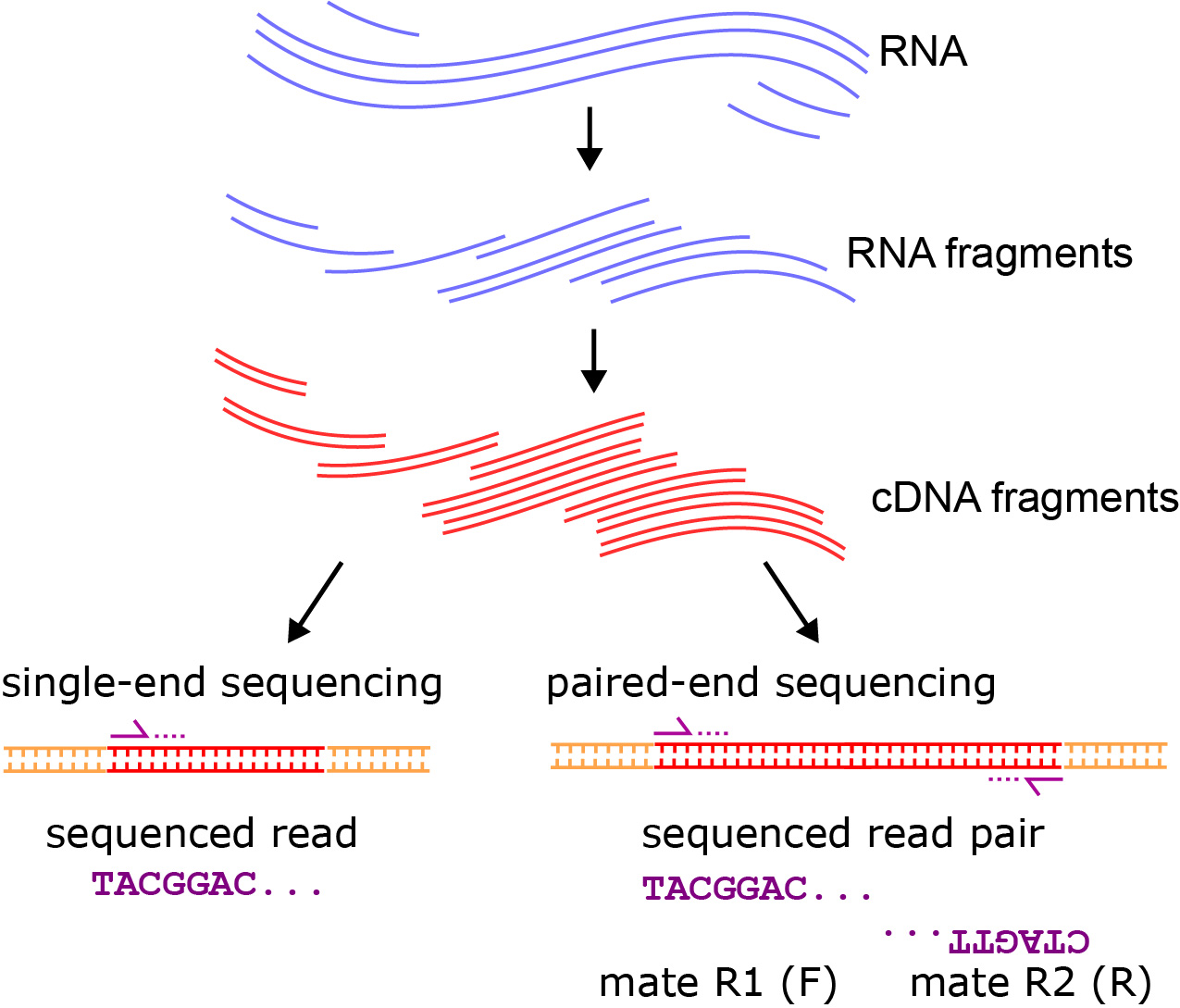
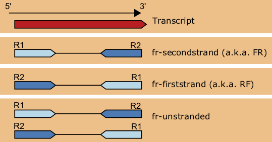
RNA deep sequencing is a method where a cDNA library is created for an RNA sample, and is sequenced using high-throughput sequencing, producing hundreds of millions of reads. Notably, there are different types of RNA-seq data sets. First, single-end reads involve the sequencing of one read per cDNA fragment, typically in the 5' to 3' direction. Paired-end reads have two reads per fragment, with the two paired-reads called "mates". Often the first mate is sequenced in the direction of transcription, and the second mate is sequenced in the opposite 3' to 5' direction. This, however, can vary on the sequencing technology used. The manual for tophat 2 (https://ccb.jhu.edu/software/tophat/manual.shtml) provides the information on Figure 6.4.
6.2.1 Single-end Sequencing
Single-end Sequencing produces one read per fragment, so it can be good for transcript quantification, but may not resolve differences in expression across splice variants or different isoforms of the same gene. Therefore, it can be good for quantifying small RNA expression, or expression at the gene-level when splice variants are not a concern.
6.2.2 Paired-end Sequencing
Paired-end Sequencing produces two reads per fragment, and where typically a fragment size distribution is known or estimated. The result is the information of both reads in a pair, often called ``mates", can be helpful in transcriptome assembly and more precise quantification of different splice variants.
Important: to get the most out of paired-end sequencing, the fragment size should be larger than the combined read length (sum of both reads).
Typically with paired end data, one receives two [latex]\texttt{fastq}[/latex] files labeled [latex]\texttt{R1}[/latex] and [latex]\texttt{R2}[/latex]. The reads in each file correspond to pairs if they have the same read ID, excluding the possibility of the reads to be labeled [latex]\texttt{R1}[/latex] and [latex]\texttt{R2}[/latex] or possibly [latex]\texttt{\1}[/latex] and [latex]\texttt{\2}[/latex]. In practice, the library type can be determined by aligning paired reads from both the R1 and R2 [latex]\texttt{fastq}[/latex] files to the genome, and examining the relative orientation of the reads and overlapping transcripts.
6.3 Small RNA sequencing
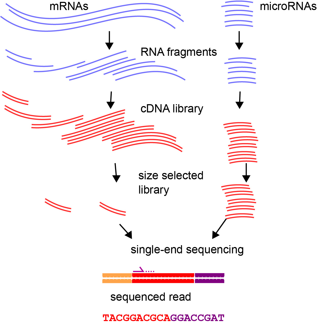
For small RNA sequencing, one typically uses single-end sequencing, which results in one read per cDNA fragment, typically in the 5' to 3' direction.
6.3.1 Adapter Trimming
Small RNA sequencing uses size-selected small RNA samples and high-throughput sequencing. Such a protocol can be used to sequence RNA species such as microRNAs and piRNAs whose endogenous mature nucleotide sequences can be shorter than the read length used to sequence them. A challenge presented here is that the 3' adapter sequence needs to be removed before aligning these sequences. For example, the program [latex]\texttt{cutadapt}[/latex] can be used to trim adapter sequences from an input FASTQ file.
cutadapt -a ATCTCGTATGCCGTCTTCTGCTTG reads.fastq > reads_trimmed.fastq
where we are trimming off the Illumina TruSeq Small RNA 3' adapter sequence.
6.3.2 Alignment of small RNA reads
In general, for both small RNAs and large RNAs, RNA-seq read alignment typically takes a FASTQ file as input, aligns to the genome, and produces a BAM or SAM file as the output.
One method for aligning reads such as small RNA reads is [latex]\texttt{bowtie}[/latex]. As one of the first methods for aligning deep sequence data, it does not allow gaps (not until bowtie2) but has other functionality such as colorspace read mapping. As a simple example, you would need to build an index of the genome that you'll be aligning to (here we are using human genome version hg38) using [latex]\texttt{bowtie-build}[/latex]. The index of the genome, much like a BLAST index created with [latex]\texttt{makeblastdb}[/latex] provides a quick look-up of genomic locations to assist with the alignment.
$ bowtie-build -f hg38.fasta hg38
Then you would align the reads (a FASTQ file) to the genome index to create an alignment (a SAM file).
$ bowtie -m 50 -l 20 -n 2 -S -q hg38 smallRNA_reads.fastq smallRNA_hg38.sam
This command takes in several options. In general, the command is the following:
$ bowtie [options]
The terms in square brackets represent optional parameters, and the angle brackets correspond to required (or highly recommended for most practical purposes) input files, but you wouldn't type the angle brackets. In this example, we have a few options specified:
$ bowtie -m 50 -l 20 -n 2 -S -q hg38 smallRNA_reads.fastq smallRNA_hg38.sam
The [latex]\texttt{"-m 50"}[/latex] specifies reads to have no more than 50 hits to the genome. The [latex]\texttt{"-l 20"}[/latex] specifies a seed length that will be used for matching to the genome. The number of mismatches to the seed is specified as [latex]2[/latex] in the [latex]\texttt{"-n 2"}[/latex] command. The [latex]\texttt{"-S"}[/latex] specifies SAM output, and [latex]\texttt{"-q"}[/latex] specifies FASTQ input.
6.3.3 Colorspace
As mentioned, [latex]\texttt{bowtie}[/latex] has the ability to align colorspace reads. Colorspace reads typically come in a [latex]\texttt{.csfasta}[/latex] file like this:
>311_5120_1770

T322302111212131102211023200

>311_5120_1780

T303223021112121311011230122
The numbers correspond to the "colors", which are not literal colors, but rather groups of dimers designated by the groups in Table 6.3.3 and in Figure 6.3.
| Dimer Groups | Color | |||
|---|---|---|---|---|
| AA | CC | GG | TT | 0=blue |
| AC | CA | GT | TG | 1=green |
| AG | CT | GA | TC | 2=yellow |
| AT | CG | GC | TA | 3=red |
The quality scores (PHRED score values) will be in an accompanying [latex]\texttt{.qual}[/latex] file:
>read1

31 31 29 31 28 29 33 22 32 28 33 32 28 30 32 30 31 ...

>read2

31 28 29 32 28 22 32 28 33 32 28 30 32 30 31 31 32 ...
Consider the sequence [latex]\texttt{T32230211}[/latex]. The sequence is determined through a process called "double interogation". Each nucleotide is determined by two color characters. Therefore, the first character, called the "primer base", gets the process going. The primer base is removed along with the adjacent color character before alignment. The rest is determined as follows. First number is [latex]3[/latex] after the [latex]\texttt{T}[/latex], leading to the only dimer in the row [latex]3[/latex] starting with [latex]\texttt{T}[/latex], which is [latex]\texttt{TA}[/latex]. Next, the number is [latex]2[/latex] after the [latex]\texttt{A}[/latex] from before. The only dimer available starting with [latex]\texttt{A}[/latex] is [latex]\texttt{AG}[/latex]. This process is continued across the sequence giving the complete sequence [latex]\texttt{TAGATTCAC}[/latex].
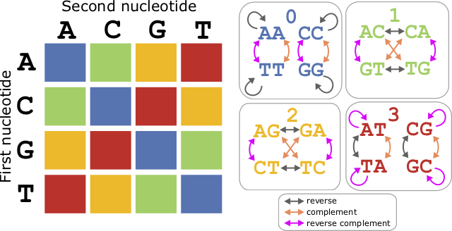
Color space also has the property that the reverse colorspace sequence is the reverse complement of the original. In the previous example, we saw that the colorspace sequence [latex]\texttt{T32230211}[/latex] encoded the DNA sequence
[latex]\texttt{TAGATTCAC}[/latex]. The reverse colorspace sequence would be [latex]\texttt{T11120322}[/latex], which encodes the reverse complement [latex]\texttt{TGTGAATCT}[/latex]. This rule holds accept for the the first character, which is the priming base. Note that both colorspace sequences also had an additional number at the beginning ([latex]3[/latex] for the first one, and [latex]1[/latex] for its reverse complement) which does not work with this reverse/reverse complement rule.
6.3.4 Quantifying small RNA Expression
For small RNA sequencing, the length is less of a concern. For example, with mature microRNAs, whether it is 18 or 25nt, you typically sequence one read per fragment. This fact suggest that small RNA reads don't need to be normazlied by the length. Therefore, for a microRNA [latex]m[/latex] with [latex]R_m[/latex] reads mapping to it out of [latex]N[/latex] total mapped reads, we would compute the expression [latex]RPM_m[/latex] as
[latex]{\label{RPMeq} RPM_m = \frac{R_m 10^6}{N }}[/latex]
(6.1)
With the module [latex]\texttt{pysam}[/latex], you can load a BAM file with the following command:
import pysam

bam = pysam.AlignmentFile("smallRNA_hg38.bam", "rb")
In this command, the "rb" term specifies "read" and "bam". If it was a SAM file, you would just use "r". You can retrieve the reads overlapping a genomic location with a command like this:
miR_count = bam.count(chrom,start,end)
Where [latex]\texttt{chrom,start,end}[/latex] are a predefined set of variables that could have been read in from a GFF file similar to Lab 6. For this function, the chromosome is a string, and the start ad stop are both ints. These ints behave like normal python boundaries, with start 0-based and the end being 0-based non-inclusive.
A better method of counting the microRNAs might also check the strand of the read.
import pysam

bam = pysam.AlignmentFile("smallRNA_hg38.bam", "rb")
chrom,start,end,strand = location
miR_count = 0

for read in bam.fetch(chrom,start,end):

    if read.is_reverse:

        if strand == '-':

            miR_count += 1

    else:

        if strand == '+':

            miR_count += 1
6.4 Long RNA sequencing
The sequencing of long RNAs, such as mRNAs and long non-coding RNAs (lncRNAs) requires long read sequencing, or simply called "RNA-seq". Single-end Sequencing produces one read per fragment, so it can be good for transcript quantification, but may not resolve differences in expression across splice variants or different isoforms of the same gene. Therefore, it can be good for quantifying small RNA expression, or expression at the gene-level when splice variants are not a concern.
6.4.1 Quality Trimming
It is good practice to trim off low-quality nucleotides from the reads based on the PHRED score. Similar to adapter trimming, this will improve the alignment.
$ fastq_quality_trimmer -t 30 -l 18 -i input_reads.fastq -o output_trimmed_reads.fastq
Is the PHRED score threshold specified by [latex]\texttt{"-t 30"}[/latex] a good one? The [latex]\texttt{"-l 18"}[/latex] threshold specifies that trimmed reads less than 18nt should be discarded.
6.4.2 Paired-end Library Types
The different arrangements of paired-end reads depticted in Figure 6.4. In practice, the library type can be determined by aligning paired reads from both the R1 and R2 fastq file to the genome, and examining the relative orientation of the reads and overlapping transcripts.
6.4.3 Methods of Read Alignment
The first step of an RNA-seq analysis is aligning the reads to the genome. Actually, there are approaches to RNA-seq without a genome discussed in section 6.4.6. For organisms with an assembled genome, the typical approach is to align the reads to the genome. There are many different programs to do this, with different features. For eukaryotic organisms, it is important that the alignment allows for gaps corresponding to introns. Another important consideration is the number of mismatches allowed in the alignment. For a highly polymorphic genome, for example, one would want to increase the number of allowed mismatches under the assumption that the transcripts sequenced could be transcribed from a slightly different genome.
RNA-seq read alignment typically takes a FASTQ file as input, aligns to the genome, and produces a BAM or SAM file as the output.
Methods for aligning RNA-seq reads include [latex]\texttt{hisat}[/latex] and [latex]\texttt{tophat}[/latex], although [latex]\texttt{hisat2}[/latex] is considered the most updated software. These programs allow gaps and both are derived from [latex]\texttt{bowtie2}[/latex].
Alignment with [latex]\texttt{hisat2}[/latex]
The first step of aligning is to have an index of the genome. As with bowtie, you would need to build an index of the genome that you'll be aligning to (here we are using human genome version hg38) using [latex]\texttt{hisat2-build}[/latex]. Note that the index files created here won't be compatible with [latex]\texttt{bowtie}[/latex] and vice versa.
$ hisat2-build hg38.fasta hg38
Then you would align the reads (a FASTQ file) to the genome index to create an alignment (a SAM file) using [latex]\texttt{hisat2}[/latex].
$ hisat2 -q --rna-strandness F -x hg38 -u RNAseq_reads.fastq -S RNAseq_hg38.sam
This command takes in several options. In general, the command is the following:
$ hisat2 [options] -x -u -S
Where the square bracket terms are optional, and the angle brackets are required (or highly recommended for most practical purposes). In this example, we have a few options specified:
$ hisat2 -q --rna-strandness F -x hg38 -u RNAseq_reads.fastq -S RNAseq_hg38.sam
The [latex]\texttt{"--rna-strandness"}[/latex] specifies that the reads are sequenced in the direction of transcription. It could also be [latex]\texttt{R}[/latex] or if not stated would assume unstranded reads by default. The [latex]\texttt{"-q"}[/latex] specifies FASTQ input, but this is the default so not strictly needed. Other options could include [latex]\texttt{--max-intronlen 100000}[/latex] if you wanted to keep intronic gaps less than 100kb.
Alignment with [latex]\texttt{tophat}[/latex]
As an example of aligning reads to the genome, let's consider [latex]\texttt{tophat}[/latex], which is part of the Tuxedo suite. For the other steps of the RNA-seq analysis pipeline we will also examine parts of the tuxedo suite pipeline.
In the case of [latex]\texttt{tophat}[/latex], which uses bowtie2 for the alignment, the creation of the index is based on the Burrows-wheeler transform. The index of the genome consists of multiple files, but each has the same prefix, or "file base" as an input. For example, with the mouse genome [latex]\texttt{mm10.fasta}[/latex] that has a file base [latex]\texttt{mm10}[/latex], we will have the six files [latex]\texttt{mm10.1.bt2}[/latex], [latex]\texttt{mm10.2.bt2}[/latex], [latex]\texttt{mm10.3.bt2}[/latex], [latex]\texttt{mm10.4.bt2}[/latex], [latex]\texttt{mm10.rev.1.bt2}[/latex], [latex]\texttt{mm10.rev.2.bt2}[/latex].
So, using default parameters, aligning with [latex]\texttt{tophat}[/latex] would be performed by the following command:
$ tophat -o reads_mm10_tophat mm10 reads.fastq
where the [latex]\texttt{-o}[/latex] option species the output directory where the output files are going to go. Probably the most important of the output files in this directory is the BAM file called [latex]\texttt{accepted\_hits.bam}[/latex]. This file contains a sorted record of the alignment information. There are other files created such as log files that could provide useful information for tracking down issues if something goes wrong. Also among these output files is [latex]\texttt{junctions.bed}[/latex], which provides a BED file of all splice junctions identified, and the number of reads that span that particular junction.
Of course, we don't always want to run [latex]\texttt{tophat}[/latex] with default parameters. For example, we might want to align with a reference annotation, such that only gaps are considered that correspond to gaps in an input GTF file. To achieve this, we would use the following command:
$ tophat -o reads_mm10_tophat --no-novel-juncs -G ensembl_mm10.gtf mm10 reads.FASTQ
Here we have specified to not include any novel junctions with the [latex]\texttt{--no-novel-juncs}[/latex] flag. Required with this flag is to specify a GTF file with the [latex]\texttt{-G}[/latex] flag. In this case we have specified an annotation from Ensembl for mm10.
We may consider adding to this a command to specify the number of mismatches (the default is 2). This can be changed with the [latex]\texttt{-N/--read-mismatches}[/latex] flag.
Quantifying Expression
Gene expression studies measure the expression levels of genes by attempting to quantify the number of mRNA transcripts per gene. There are a number of ways to compute gene expression, with varying accuracy and different pros and cons.
6.4.4 Quantifying Expression with Microarrays
Microarrays allow for high-throughput measurement of gene expression through the use of hybridization probes. The probes are DNA sequences that are complementary to the transcripts that you would like to measure (or more precisely the cDNA created from the transcripts). Because of the requirement of probes to detect the gene expression, one or more probes for each gene needs to be designed. This puts a constraint on the genes that one can detect. Also, different hybridization energies can complicate the analysis in some cases, as this would need to be controlled for.
6.4.5 Quantifying Expression with RNA-seq
When quantifying expression with RNA-seq, it is important to consider a normalization of the data that best controls for the fact that sequencing depth may vary from experiment to experiment, and gene lengths are highly variable. Longer genes generate more fragments, and hence result in more reads per physical mRNA molecule. One method that has these properties is RPKM, which stands for Reads Per Kilobase of gene length per Million reads mapped. For a gene [latex]g[/latex] of lenxth [latex]L_g[/latex], with [latex]R_g[/latex] reads mapping to it out of [latex]N[/latex] total mapped reads, we would compute the expression [latex]RPKM_g[/latex] with
[latex]{\label{RPKMeq} RPKM_g = \frac{R_g 10^9}{L_g N }}[/latex]
(6.2)
Taking this idea further, another measure of expression is the FPKM, or Fragments Per Kilobase of gene length per Million reads mapped. Here, the fragment refers to the cDNA fragment from which the read was sequenced. For example with paired-end reads, we have two reads per fragment. If one of the mates was of poor quality or did not map, the reads would underestimate the number of fragments mapping to this location. For example, when aligning with [latex]\texttt{tophat}[/latex], there is an option [latex]\texttt{"--no-discordant"}[/latex], which would only allow reads where both mates properly map the the same chromosome or scaffold. When this option is not used, there are cases where one fragment corresponds to one read (either [latex]\texttt{R1}[/latex] or [latex]\texttt{R2}[/latex]) or both reads. When the [latex]\texttt{--no-discordant}[/latex] option is used, each fragment corresponds to two reads.
Measuring Differential Expression with RNA-seq
The program [latex]\texttt{cuffdiff}[/latex] is part of the [latex]\texttt{cufflinks}[/latex] software package, and it computes expression values of genes and identifies significantly differentially expressed genes. with default parameters, we can run cuffdiff to compare the expression of two RNA-seq experiments with the following command (input on one line):
$ cuffdiff -o treatment_vs_control -L treatment,control \\

    ensembl_mm10.gtf treatment_mm10/accepted_hits.bam control_mm10/accepted_hits.bam
So we note that in this case it is required that we specify a GTF annotation file to use to use such that the expression of the genes annotated in this file are quantified. Furthermore, we need two BAM files, presumably both aligned with Tophat using the same parameters. The [latex]\texttt{-L}[/latex] parameter specifies "labels" for the BAM file compared, such that the output files will use these in the file header. For each BAM file, we could also give SAM files, or a comma-separated list of BAM files corresponding to individual replicates for that experiment. The [latex]\texttt{-o}[/latex] command specifies the output directory in which the results will be print. Lastly, the [latex]\texttt{"\\"}[/latex] is used to split the command on two lines here, but is not necessary to type.
The results of a cuffdiff computation is a set of many files. Among them are differential expression files called [latex]\texttt{.diff}[/latex] files. There are files for the genes and for the isoforms for the genes given by [latex]\texttt{gene\_exp.diff}[/latex] and [latex]\texttt{isoform\_exp.diff}[/latex] files respectively. These [latex]\texttt{diff}[/latex] files contain the information on the genomic location of the transcript, as well as FPKM values for the samples compared. Furthermore, it has the log fold change of these expression values, as well as output from a statistical test to identify significantly differentially expressed genes.
Intersection Count, Union Count, and the True Expression
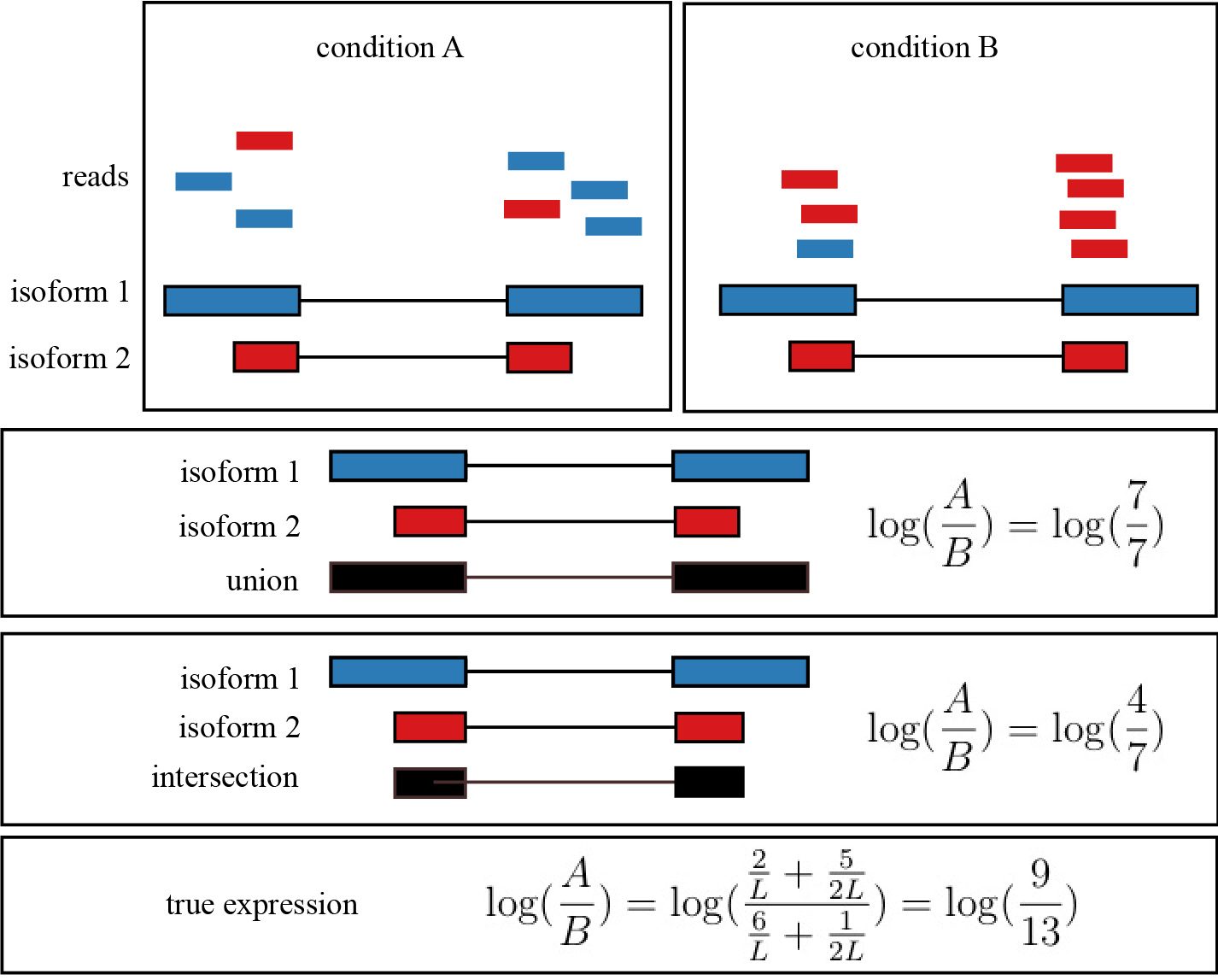
When counting reads that overlap a gene model, there are different approaches to quantifying the expression of a gene with multiple transcript isoforms. For example, the intersection count would take the expression of all exons that are common to each isoform in a particular gene. The union count take the perspective of counting the reads that overlap the union of all exons for a particular gene. As pointed out in Trapnell et al. 2013, there are issues with both of these models. Figure 6.5 demonstrates a scenario with both the intersection and union count models fail to accurately depict the expression of a gene.
6.4.6 Transcriptome Assembly
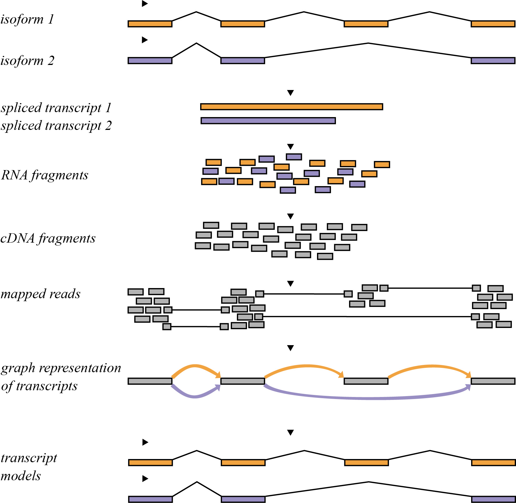
Transcriptome assembly is the process by which the aligned reads are compiled into transcript models that best represent the read data. At minimum, a transcript model must consist of reads that map to that location. Introns must be supported by a gapped alignment that spans the intronic region, typically further requiring that the donor and acceptor sites are present at the start and end of the intron (GU on the 5' end and AG on the 3' end of the intron). We may optionally want to assemble a transcriptome for an RNA-seq experiment when we don't have a transcriptome annotation available. We may also want to perform this step when none is available. A schematic of how this process is performed is depicted in Figure 6.6
Stringtie
In general, running [latex]\texttt{stringtie}[/latex] uses commands of the following form:
$ stringtie [options] RNAseq_reads.bam -G human_RefSeq.gtf -o transcriptome_v2.gtf
Where the square bracket terms are options. In fact, the [latex]\texttt{"-G"}[/latex] is also optional, but builds the transcriptome assembly using the provided GTF file as a guide. Other options include for example [latex]\texttt{"-j 2"}[/latex] would require 2 reads to build a splice junction, rather than the default value of [latex]1[/latex].
You can also use stringtie to combine and merge several GTF files into one. There are two ways to do this.
$ stringtie --merge [options] gtf_file_list.txt
Where [latex]\texttt{gtf\_file\_list.txt}[/latex] is a list of GTF files. Alternatively, you can specify the GTF files in a series after the command:
$ stringtie --merge [options] human_transcripts1.gtf human_transcripts2.gtf
Cufflinks
The next step of the Tuxedo suite that corresponds to transcriptome assembly is [latex]\texttt{cufflinks}[/latex]. This can be run with default parameters with the following command:
$ cufflinks reads_mm10_tophat/accepted_hits.bam
where we have specified the BAM file produced from the previous [latex]\texttt{tophat}[/latex] commands. We may want to add a reference annotation to our command. This may seem counter-intuitive since the purpose is to create our own new transcriptome assembly, but doing so allows cufflinks to assign gene names corresponding to known gene names in the annotation file. We can do this with the updated command:
$ cufflinks -g ensembl_mm10.gtf reads_mm10_tophat/accepted_hits.bam
Note that we are specifying the same GTF file as before, but cufflinks uses a lower-case "-g", whereas [latex]\texttt{tophat}[/latex] uses an upper-case "-G". We may want to consider is to make the alignment run "quietly", by reducing the number of printed messages with the [latex]\texttt{-q}[/latex] option. Another option worth considering is the [latex]\texttt{-I}[/latex] option (capital i), which specifies the maximum intron length, or gap-length to consider. Restricting this can occasionally remove artifacts since the default is [latex]300,000[/latex]bp.
Transcriptome Assembly without a Reference Genome
There are approaches to assemble a transcriptome and quantify gene/transcript expression without a reference genome. Prominent among them is the suite called "Trinity", which consists of three pieces of software, as the name suggests [54].
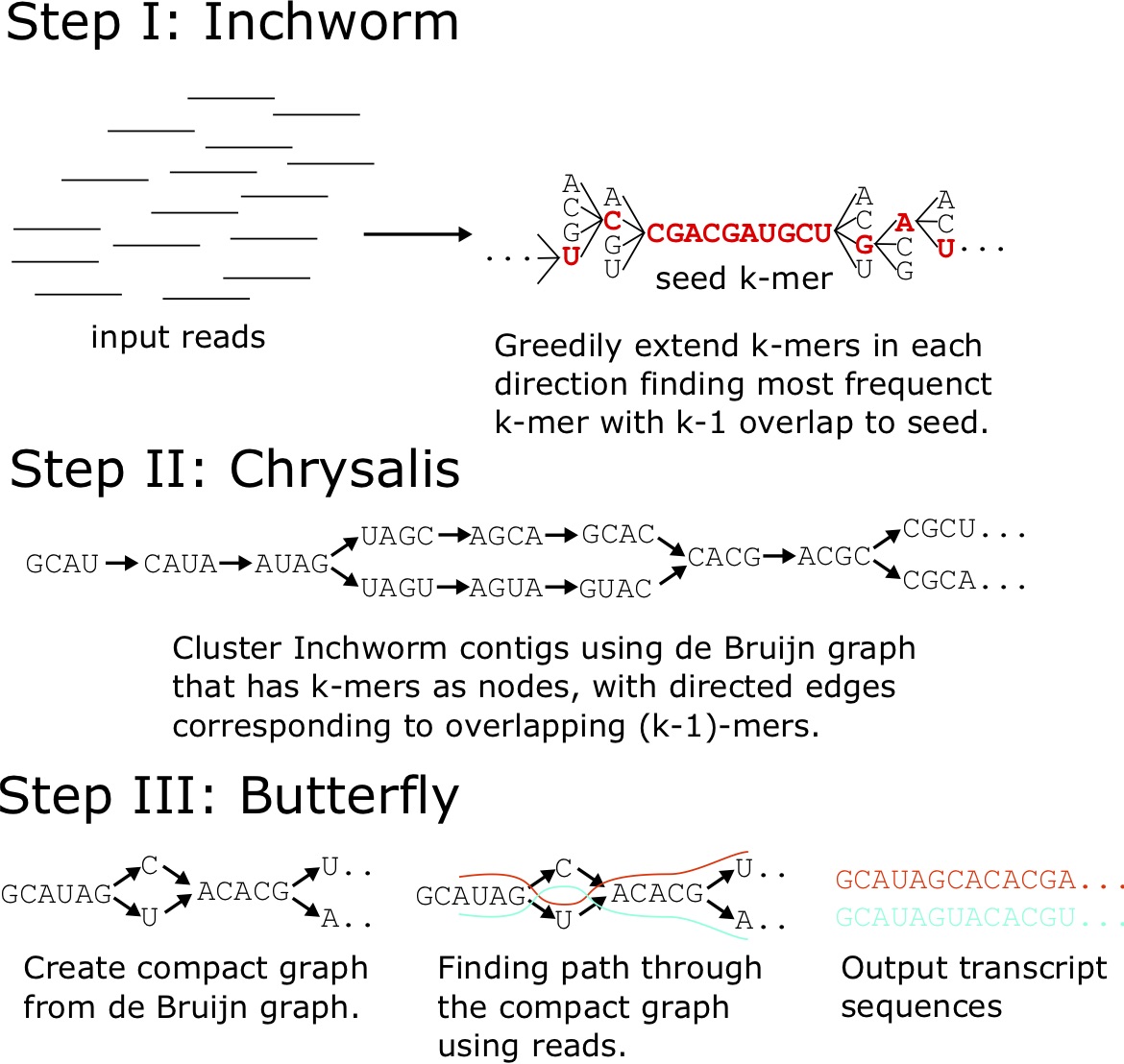
The software components of Trinity work in series to create a transcriptome assembly in three steps (Figure 6.7). First, [latex]\texttt{Inchworm}[/latex] clusters reads by common [latex]K[/latex]-mers (subsequences of length [latex]K[/latex]). Next, [latex]\texttt{Chrysalis}[/latex] clusters contigs into components consisting of matched [latex]K[/latex]-mers, and builds a de Bruijn graph from these components. In the last step, [latex]\texttt{Butterfly}[/latex] assembles transcript models from the de Bruijn graph [54].
6.5 Single-Cell Transcriptomics
While traditional RNA-seq measures gene expression on many, typically heterogeneous cells, single-cell RNA-seq (scRNA-seq) is a method for measuring gene expression in hundreds of individual cells [55]. While these methods do reduce heterogeneity compared to bulk measurements, they do have a large amount of technical noise [56].
6.6 Transcription Initiation
Transcription Initiation is a remarkable process, because it is very much a needle-in-a-haystack phenomena. Somehow, the cell is able to pinpoint specific single-nucleotide positions out of the genome, and use these specific positions as the start of a transcript. This first nucleotide that is transcribed is called the Transcription Start Site (TSS).
In many cases, transcription initiation begins with the recognition of the core promoter, which is a collection of binding sites that direct the initiation of transcription. In eukaryotes, RNA polymerase II does not directly recognize the core promoter sequences. Instead, a collection of proteins called transcription (activation) factors (TAFs) mediate the binding of RNA polymerase and the initiation of transcription. Only after certain transcription factors are attached to the promoter does the RNA polymerase bind to it. The completed assembly of transcription factors and RNA polymerase bind to the promoter, forming a transcription initiation complex.
In prokaryotes, transcription begins with the binding of RNA polymerase to the promoter in DNA. At the start of initiation, the core enzyme is associated with a sigma factor that aids in finding the appropriate -35 and -10 base pairs upstream of promoter sequences. When the sigma factor and RNA polymerase combine, they form a holoenzyme.
6.6.1 Methods of Mapping Transcription Start Sites (TSSs)
There are many methods that have been developed for the mapping of transcription start sites. Most of these methods rely on the biochemistry of the 5' end of transcribed RNA.
Cap Analysis of Gene Expression (CAGE)
CAGE sequencing begins by capping the 5' ends of small transcript fragments, which are then extracted, reverse transcribed to DNA, PCR amplified and sequenced. CAGE reads tend to map at the transcription start site of genes , but in practice do map at and around these locations. The CAGE technique precedes that of high-throughput sequencing and was used before then, but has benefited from the depth associated with new sequencing techniques.
Rapid Amplification of edna Ends (RACE)
In RACE, a cDNA copy of the mRNA is produced through reverse transcription, PCR amplification of the cDNA copies. There are different methods for 5' RACE and 3' RACE, resulting in the proper mapping of both the 5' end and the 3' end of genes. 3' RACE uses the poly(A) tail of genes for priming during the reverse transcription. 5' RACE uses a gene-specific primer that recognizes a known region of the gene of interest.
Database of Transcription Start Sites (DBTSS)
The Database of Transcription Start Sites (DBTSS) is a resource of experimentally mapped transcription start sites, through a method called TSS-seq, and is primarily focused on human and mouse, but contains other species. This database now contains 491 million TSS tag sequences collected from 20 different human tissues and 7 different human cell cultures. The DBTSS can be accessed at http://dbtss.hgc.jp/.
The TSS-seq method ligates the Illumina sequencing adapter to the 5' cap site of the mRNA, performs full-length cDNA creation, and high-throughput sequencing. The uniquely mapping sequencing reads are then mapped to the genome, and clustered into [latex]500[/latex]bp bins. TSCs overlapping internal exons are then removed, and each cluster is either associated with the most likely RefSeq transcript, or labeled as intergenic
6.7 Transcription
Transcription is carried out by RNA Polymerase, which makes a RNA copy of the template strand of a gene's DNA sequence. Measurements of the binding of RNA Polymerase II (Pol II) to genes has revealed that not all genes have the same binding profiles over their promoter regions and gene bodies.
6.7.1 Measuring RNA Polymerase binding: Pol II ChIp-seq
Pol II ChIP-seq provides a signal the binding of Pol II to the genomic DNA. It measures the recruitment of Polymerase to the genome, but the Ser5 of the Pol II complex needs to be phosphorylated for transcription to begin. Therefore, many of these protocols use antibodies that specifically recognize the Ser5-Phosphorylated form of Pol II as well as other forms.
Briefly, chromatin samples are crosslinked and sonicated into fragments. Chromatin is immunoprecipitated with a RNA Pol II antibody, or cocktail of antibodies that recognize different forms of Pol II. DNA fragments are then isolated and sequenced with HTS. These reads are then mapped to the genome, and the number of reads that map to a particular genomic region is indicative of the time that Pol II spends binding to that region.
6.7.2 RNA Polymerase II Stalling
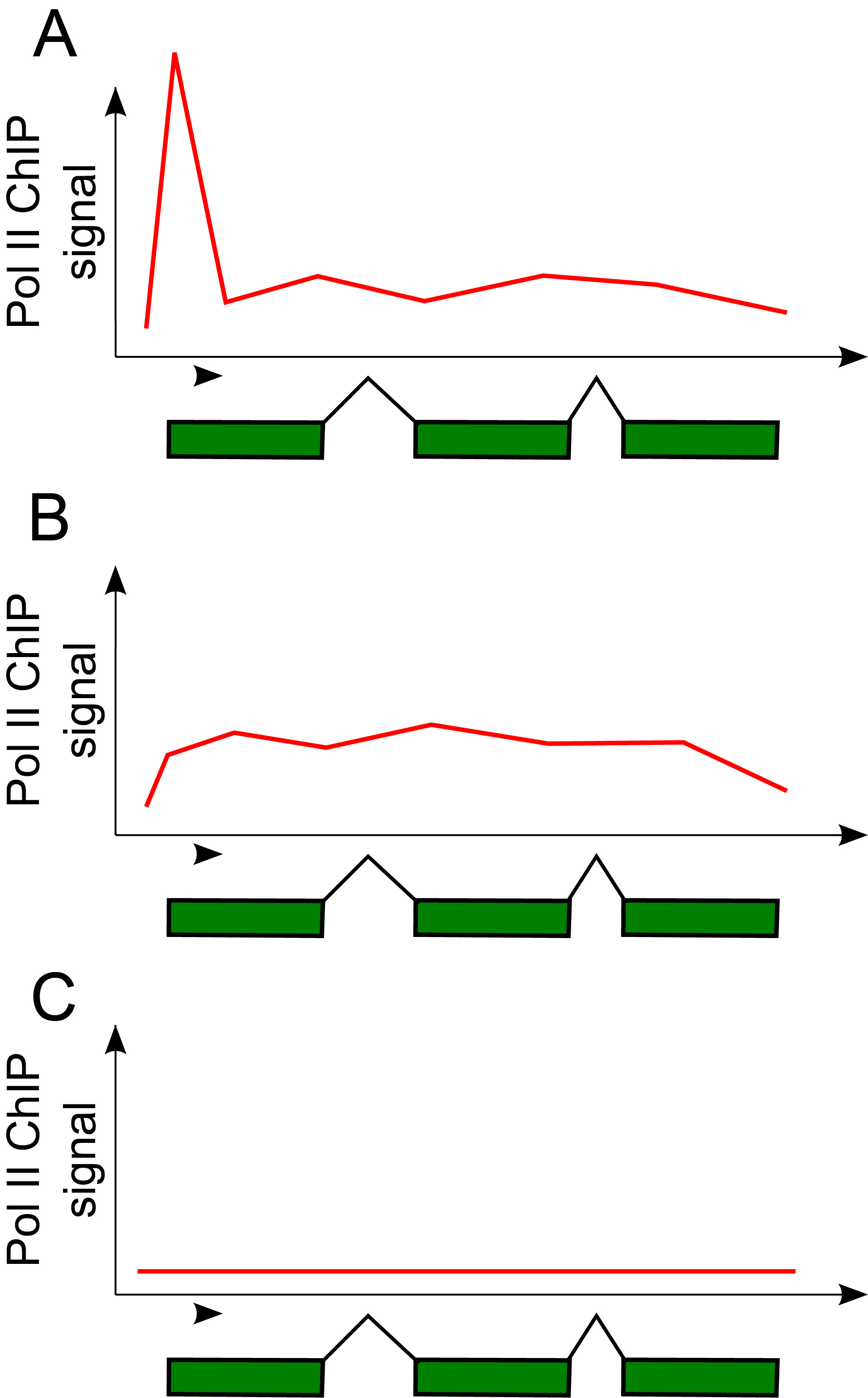
One of the phenomena observed using Pol II ChIP-seq is stalling (Pol II Stalling) [57]. Stalled Pol II is capable of quickly responding to input signals because the transcript is already initiated, and hence is called "poised" [58] for rapid activation. Pol II Stalling is associated with a greater proportion of Pol II ChIP-seq reads at and around the TSS of genes compared to the gene body. For a Pol II signal given by [latex]S(i)[/latex] for position [latex]i[/latex] of the genome, The state of being stalled is defined by a large stalling index:
[latex]SI = \frac{max_{TSS} \{ S(i) \} }{median_{gene} \{ S(i) \}}[/latex]
where [latex]max_{TSS} \{ S(i) \}[/latex] indicates the maximum signal value [latex]S(i)[/latex] within some distance of the TSS of the gene, and [latex]median_{gene} \{ S(i) \}[/latex] indicates the median signal value within the gene body [57].
6.8 Elongation
Elongation is characterized by the release of Pol II from the promoter, and the production of RNA transcripts. In mammalian genes, the Pol II elongation rates are about 0.5kb per minute in the first few kilobases, and increases to 2-5kb per minute after 15kb [59].
6.8.1 Measuring Nascent Transcription: GRO-seq
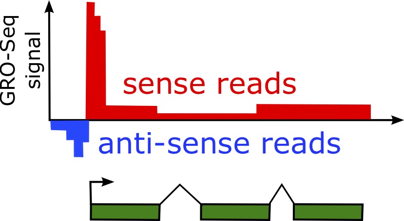
While Pol II ChIP-seq measures DNA-associated Pol II, Global Run-On Sequencing (GRO-seq) measures transcriptionally engaged Pol II, by detecting nascent RNA transcripts. GRO-seq involves a nuclear run-on experiment on a genome-wide scale, where engaged Pol II incorporates bromo-tagged nucleotides, and is followed by RNA isolation and deep sequencing [60].
6.8.2 Divergent Transcription
One of the phenomena observed using Global Run-On sequencing (GRO-seq) is that of divergent transcription [61]. Divergent transcription is characterized by nascent transcripts associated with both the sense and anti-sense strand of the gene.
6.9 Lab 7: RNA-seq
The data for this project was taken from a paper by Kurasz et al., which describes a study of gene expression in Salmonella enterica serovar Typhimurium and the effect of nucleic acid damage induced by mitomycin (MMC), which is a chemotherapy drug, and other compounds [62]. We will look at the MMC data in this project. I'm assuming you're working in a new directory called [latex]\texttt{Lab7}[/latex].
Due to the large amount of data generated, I have some streamlined versions of these files to make it possible to complete this lab in less than an hour.
6.9.1 Step 1: Download the genome and build a hisat2 index
First thing we should do is download the genome for Salmonella. For reference, I found this by searching NCBI in the "Assembly" section and found this link here: https://www.ncbi.nlm.nih.gov/assembly/?term=Salmonella+Typhimurium. I renamed the file and made it available at this link:
$ wget http://hendrixlab.cgrb.oregonstate.edu/teaching/salmonella_genome.fasta
Next, we should build a [latex]\texttt{hisat2}[/latex] index with the following command:
$ hisat2-build salmonella_genome.fasta sal
In this command, I have used the filebase "sal", which is specified as the second argument to [latex]\texttt{hisat2}[/latex] above, but you could call it what you want and change the subsequent commands accordingly. Note that several files are created as a result:
$ ls sal.*

sal.1.ht2 sal.2.ht2 sal.3.ht2 sal.4.ht2 sal.5.ht2 sal.6.ht2 sal.7.ht2 sal.8.ht2
6.9.2 Step 2: Download the FASTQ files and align with hisat2
First, we will download the FASTQ file. I found this experiment on GEO here: https://www.ncbi.nlm.nih.gov/geo/query/acc.cgi?acc=GSE82167}. As a side note, what I did was go to the "Samples" section, expanded that section, clicked the links to find the "SRR..." IDs for samples. I ran a command like this (but please don't run this because the original files are too big!):
$ ~/sratoolkit.2.9.4-centos_linux64/bin/fastq-dump -A SRR3621123 >& SRR3621123.err

$ ~/sratoolkit.2.9.4-centos_linux64/bin/fastq-dump -A SRR3621125 >& SRR3621125.err
These commands assume you have installed the SRA toolkit in your home directory, and are using version 2.9.4, and are using CentOS; please alter these as needed. To make this more feasible in class, I have created the following shortened version of the resulting files:
$ wget http://hendrixlab.cgrb.oregonstate.edu/teaching/salmonella_ctrl.fastq

$ wget http://hendrixlab.cgrb.oregonstate.edu/teaching/salmonella_MMC.fastq
Question: How many lines are in these files and how many reads does it have?
We might want to quality trim these files, as well as remove any potential adapters. You can trim the files with [latex]\texttt{skewer}[/latex] using the commands:
$ skewer -x AGATCGGAAGAGCACACGTCTGAACTCCAGTCAC -q 30 -Q 30 salmonella_ctrl.fastq -o salmonella_ctrl

$ skewer -x AGATCGGAAGAGCACACGTCTGAACTCCAGTCAC -q 30 -Q 30 salmonella_MMC.fastq -o salmonella_MMC
For this command, it is requiring a PHRED score of 30 for both the 3' end as well as the average score. Meaning, nucleotides will be removed from the 3' end if they are lower quality than 30, and will discard reads with an average score less than 30.
The alignment itself is done with [latex]\texttt{hisat2}[/latex] using mostly default options to create a SAM file as the output.
$ hisat2 -x sal -U salmonella_ctrl-trimmed.fastq -S salmonella_ctrl.sam

$ hisat2 -x sal -U salmonella_MMC-trimmed.fastq -S salmonella_MMC.sam
6.9.3 Step 3: Convert SAM to BAM, sort, and index the files
In order for cuffdiff to run properly, we need to sort and index the files. SAM will work actually, but it needs to be sorted. Perhaps the easiest and fastest thing is do do this with samtools, which is like a "Swiss Army knife" for SAM and BAM files. First, convert to BAM using samtools
$ samtools view -b -S -o salmonella_ctrl.bam salmonella_ctrl.sam

$ samtools view -b -S -o salmonella_MMC.bam salmonella_MMC.sam
Next, we sort and index these files:
$ samtools sort salmonella_ctrl.bam salmonella_ctrl.sort

$ samtools index salmonella_ctrl.sort.bam

$ samtools sort salmonella_MMC.bam salmonella_MMC.sort

$ samtools index salmonella_MMC.sort.bam
6.9.4 Step 4: Identify differentially expressed genes with Cuffdiff.
To do this, you'll need to download the GFF file for the organism.
$ wget http://hendrixlab.cgrb.oregonstate.edu/teaching/salmonella.gff
Please read more information on the options of cuffdiff, check here: http://cole-trapnell-lab.github.io/cufflinks/cuffdiff/index.html. We are going to run a basic version here, and the only option we are setting is to create a label for the output file columns with meaningful labels.
$ cuffdiff -L WT,MMC salmonella.gff salmonella_ctrl.sort.bam salmonella_MMC.sort.bam
Do you find any differentially expressed genes? These will correspond to those significant at an FDR of 0.05, by default. They make this easy to putting a "yes" on the last column for genes that are significant.
$ grep yes gene_exp.diff
Do these genes make sense given the paper, and can you find information about their function at NCBI?
You can look for enriched functional annotations using the "GO Enrichment" tool at http://geneontology.org/. GO Terms are part of a controlled vocabulary for gene functions. Salmonella is an available organism on this page, which enables us to study gene enrichment associated with the differentially expressed genes from this experiment. By extracting the gene IDs, you could paste them into this GO Enrichment tool, and compute enriched functional categories.

