Chapter 3: Sequence Alignments
Biological sequences evolve through a process of mutation and natural selection. By comparing two sequences, we can determine whether two sequences have a common evolutionary origin if their similarity is unlikely to be due to chance. Before we get into how this is done, we must also consider that there are many types of evolutionary relationships among sequences.
First, there is similarity, which fits the intuitive meaning of the degree of resemblance between two sequences. We might use the term identity to refer to more exact situations, such as the state of possessing the same subsequence. One often quantifies the percent identity between two sequences. The term homology refers to the state of sharing a common evolutionary origin. We say two sequences are homologous if they have a common ancestor. There are two types of homology. First, orthology refers to the state of being homologous sequences that arose from a common ancestral gene during speciation. Second, paralogy refers to the state of being homologous sequences that arose from a common ancestral gene from gene duplication.
Sequence alignment is the process of arranging the characters of a pair of sequences such that the number of matched characters is maximized. We can describe the alignment between two sequences with the following notation:
GCGTAACACGTGCG--

 | ||| ||||||

AC--AACCCGTGCGAC
The vertical bars [latex]\texttt{"|"}[/latex], or pipes, represent matching characters. Gaps, indicated by the dash [latex]\texttt{"-"}[/latex] are inserted in between characters in place of missing characters to optimize the number of matches. It is critical that sequence alignments are viewed in a monospace font, such as Courier, so that the width of characters don’t offset the alignment.
3.1 Alignment Algorithms and Dynamic Programming
One of the first attempts to align two sequences was carried out by Vladimir Levenstein in 1965, called “edit distance”, and now is often called Levenshtein Distance. The edit distance is defined as the number of single character edits necessary” to change one word to another. Initially, he described written texts and words, but this method was later applied to biological sequences. One of the most commonly used algorithms for computing the edit distance is the Wagner-Fischer algorithm, a Dynamic Programming algorithm.
Dynamic Programming optimally phrases the full problem as the optimal solution to the smaller pieces (sub-problems). The overall problem can then be expressed as a composition of the sub-problems. In addition to the Wagner-Fischer algorithm, numerous other dynamic programming algorithms have been developed for aligning biological sequences including the Needleman-Wunsch [22] and Smith-Waterman Algorithms [23].
3.1.1 Needleman-Wunsch Algorithm
The Needleman-Wunsch Algorithm is a global alignment algorithm, meaning the result always aligns the entire input sequences [22]. Later on in section 8.1 we will define a scoring matrix for protein alignment, but for nucleotide sequences, we often use a simpler scoring matrix such as
[latex]\begin{aligned} S_{a,b} = \begin{cases} 1, & \text{if } a=b \\ -1, & \text{if } a \ne b \end{cases} \end{aligned}[/latex]
(3.1)
In addition to a scoring matrix, we also need to define penalties for gaps. The most common gap penalty is the linear gap penalty, defined as
[latex]c_L(d) = G d,[/latex]
which is just proportional to the length [latex]d[/latex] of the gap by a parameter [latex]G \lt 0[/latex]. A more complicated approach is an “affine gap penalty”, which penalizes opening a gap by one parameter, and extending the gap by another parameter. For example, such a gap penalty can by defined by
[latex]c_A(d) = G + (d-1) E[/latex]
which includes a gap open parameter [latex]G[/latex] and a gap extension parameter [latex]E[/latex]. In practice, an affine gap penalty is much more difficult to compute.
Dynamic programming for sequence alignments begins by defining a matrix or a table, to compute the scores. For example, let’s consider aligning the nucleotide sequences [latex]x = \texttt{CAGCTAGCG}[/latex] and [latex]y = \texttt{CCATACGA}[/latex]. For Needleman-Wunsch, let’s define a matrix [latex]F[/latex], such that the terms [latex]F_{i,j}[/latex] correspond to the score of aligning the subsequences [latex]x[1..i][/latex] and [latex]y[1..j][/latex]. We proceed from the upper left of this matrix at [latex]F_{0,0}[/latex], and fill in the matrix as we move from left to right and from top to bottom. Here the rows of [latex]F[/latex] will correspond to the positions of [latex]x[/latex], and the columns will correspond to the positions of [latex]y[/latex].
When computing the terms of the matrix [latex]F[/latex], we need to define a set of boundary conditions, namely that the score at the boundaries is associated with the penalty all the way up to that position. This is achieved by setting [latex]F_{i,0} = i \times G[/latex] and [latex]F_{0,j} = j \times G[/latex] for [latex]1 \le i \le |x|[/latex] and [latex]1 \le j \le |y|[/latex].
We compute the terms of the matrix [latex]F[/latex] using a “recurrence relation”, such that the terms of a given cell of the matrix [latex]F[/latex] are defined in terms of the neighboring cells. Needleman-Wunsch uses the following recurrence relation:
[latex]\begin{aligned} F_{i,j} = max \begin{cases} F_{i-1,j} + G& \mbox{skip a position of }x\\ F_{i,j-1} + G& \mbox{skip a position of }y\\ F_{i-1,j-1} + S_{x[i],y[j]} & \mbox{match/mismatch}\\ \end{cases} \end{aligned}[/latex]
(3.2)
Let’s consider the result of computing the matrix [latex]F[/latex] using the scoring matrix in 3.1, and using a linear gap penalty [latex]G=-1[/latex]. The result is presented in Table 3.1.1. In this matrix, each term then corresponds to the score up to the character at that [latex]i[/latex] and [latex]j[/latex] position of the sequences [latex]x[/latex] and [latex]y[/latex] respectively. The rows will correspond to positions [latex]i[/latex] in the sequence [latex]x[/latex], and the columns will correspond to positions [latex]j[/latex] of [latex]y[/latex].
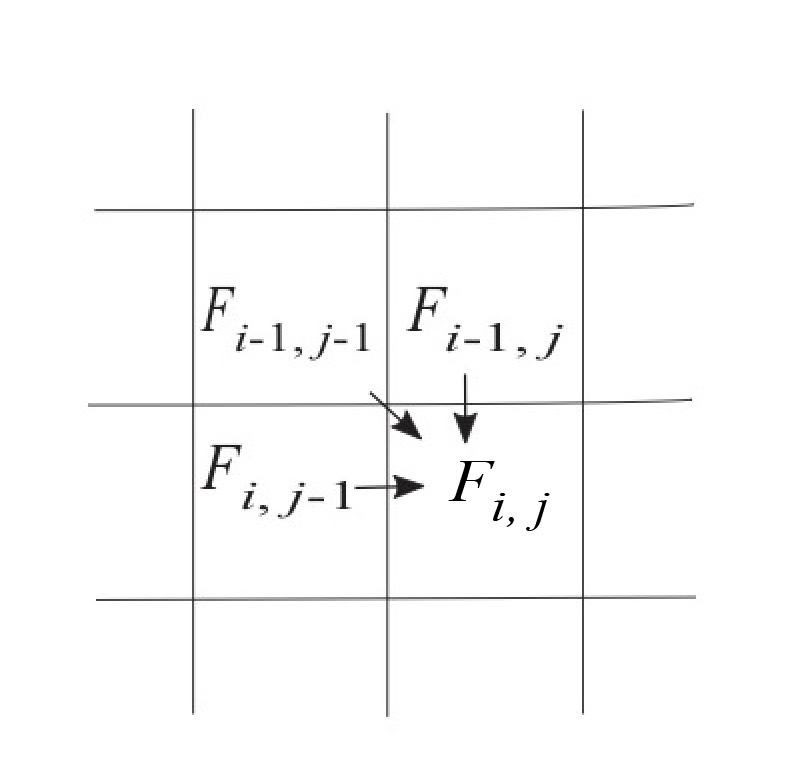
The terms [latex]F_{ij}[/latex] of the matrix [latex]F[/latex] can be filled out as is done with the following matrix, with each cell computed using the recursion relation in Equation 3.2, as depicted in Figure 3.1. The optimal path is shown in blue.
| – | – | C | C | A | T | A | C | G | A |
|---|---|---|---|---|---|---|---|---|---|
| – | 0 | -1 | -2 | -3 | -4 | -5 | -6 | -7 | -8 |
| C | -1 | 1 | 0 | -1 | -2 | -3 | -4 | -5 | -6 |
| A | -2 | 0 | 0 | 1 | 0 | -1 | -2 | -3 | -4 |
| G | -3 | -1 | -1 | 0 | 0 | -1 | -2 | -1 | -2 |
| C | -4 | -2 | 0 | -1 | -1 | -1 | 0 | -1 | -2 |
| T | -5 | -3 | -1 | -1 | 0 | -1 | -1 | -1 | -2 |
| A | -6 | -4 | -2 | 0 | -1 | 1 | 0 | -1 | 0 |
| G | -7 | -5 | -3 | -1 | -1 | 0 | 0 | 1 | 0 |
| C | -8 | -6 | -4 | -2 | -2 | -1 | 1 | 0 | 0 |
| G | -9 | -7 | -5 | -3 | -3 | -2 | 0 | 2 | 1 |
In addition to the [latex]F[/latex] matrix, it is common to keep track of a traceback matrix [latex]T[/latex], that keeps track of from where each term was computed from, in other words the maximum term in Eq 3.2. Table 3.1.1 demonstrates such a traceback matrix. One key complication is dealing with ties. One strategy is to favor adjacent matched characters as much as possible; therefore, we would favor diagonal terms before above or to the left.
| – | – | C | C | A | T | A | C | G | A |
|---|---|---|---|---|---|---|---|---|---|
| – | · | · | · | · | · | · | · | · | · |
| C | · | × | ↖ | ← | ← | ← | ↖ | ← | ← |
| A | · | ↑ | ↖ | ↖ | ← | ↖ | ← | ← | ↖ |
| G | · | ↑ | ↖ | ↑ | ↖ | ↖ | ↖ | ↖ | ← |
| C | · | ↖ | ↖ | ← | ↖ | ↖ | ↖ | ← | ↖ |
| T | · | ↑ | ↑ | ↖ | ↖ | ← | ↑ | ↖ | ↖ |
| A | · | ↑ | ↑ | ↖ | ← | ↖ | ← | ← | ↖ |
| G | · | ↑ | ↑ | ↑ | ↖ | ↑ | ↖ | ↖ | ← |
| C | · | ↖ | ↖ | ↑ | ↖ | ↑ | ↖ | ← | ↖ |
| G | ↑ | ↑ | ↑ | ↖ | ↑ | ↑ | ↖ | ← |
Finally, we have the result of the alignment. Here is the result of the Needleman-Wunsch alignment. Because it is a global alignment, the full sequence is included and the alignment ends on the first and last positions. There are, however, gaps at the first and last positions as this example illustrates.
-CAGCTAGCG-

 ||  || ||

CCA--TA-CGA
3.1.2 Smith-Waterman
n most applications we are only interested in aligning a small portion of the sequence to produce a local alignment. Furthermore, we don’t necessarily want to force the first and last residues to be aligned. Smith-Waterman is an alignment algorithm that has these properties [23].
We can define a set of boundary conditions for the scoring matrix [latex]F_{i,j}[/latex], namely that the score is [latex]0[/latex] at the boundaries so that [latex]F_{i,0} = F_{0,j} = 0[/latex] for [latex]1 \le i \le |x|[/latex] and [latex]1 \le j \le |y|[/latex]. Define the recurrence relation:
[latex]\begin{aligned} F_{i,j} = max \begin{cases} F_{i-1,j} + G& \mbox{skip a position of }x\\ F_{i,j-1} + G& \mbox{skip a position of }y\\ F_{i-1,j-1} + S_{x[i],y[j]} & \mbox{match/mismatch}\\ 0 & \mbox{zero-out negative scores} \\ \end{cases} \end{aligned}[/latex]
(3.3)
In addition to the different boundary conditions, a key difference between Needleman-Wunsch (global alignment) and Smith-Waterman (local alignment) is that whereas with the global alignment we start tracing back from the lower right term of the matrix, for the local alignment we start at the maximum value. This value corresponds to the last matched character of the optimal alignment.
| – | – | C | C | A | T | A | C | G | A |
|---|---|---|---|---|---|---|---|---|---|
| – | 0 | 0 | 0 | 0 | 0 | 0 | 0 | 0 | 0 |
| C | 0 | 1 | 1 | 0 | 0 | 0 | 1 | 0 | 0 |
| A | 0 | 0 | 0 | 2 | 1 | 1 | 0 | 0 | 1 |
| G | 0 | 0 | 0 | 1 | 1 | 0 | 0 | 1 | 0 |
| C | 0 | 1 | 1 | 0 | 0 | 0 | 1 | 0 | 0 |
| T | 0 | 0 | 0 | 0 | 1 | 0 | 0 | 0 | 0 |
| A | 0 | 0 | 0 | 1 | 0 | 2 | 1 | 0 | 1 |
| G | 0 | 0 | 0 | 0 | 0 | 1 | 1 | 2 | 1 |
| C | 0 | 1 | 1 | 0 | 0 | 0 | 2 | 1 | 1 |
| G | 0 | 0 | 0 | 0 | 0 | 0 | 1 | 3 | 2 |
The optimal score corresponds to the [latex]3[/latex] in the last row, but second to last column. The optimal path results in an alignment with four matching positions. The traceback matrix can be built while computing the alignment matrix, and all paths are halted when a score of zero is reached.
| – | – | C | C | A | T | A | C | G | A |
|---|---|---|---|---|---|---|---|---|---|
| – | · | · | · | · | · | · | · | · | · |
| C | · | ↖ | ↖ | ← | · | · | ↖ | ← | · |
| A | · | ↑ | ↖ | ↖ | ← | ↖ | ↑ | ↖ | ↖ |
| G | · | · | · | ↑ | ↖ | ↖ | ↖ | ↖ | ↑ |
| C | · | ↖ | ↖ | ↑ | ↖ | ↖ | ↖ | ↑ | ↖ |
| T | · | ↑ | ↖ | ↖ | × | ← | ↑ | ↖ | · |
| A | · | · | · | ↖ | ↑ | ↖ | ← | ← | ↖ |
| G | · | · | · | ↑ | ↖ | ↑ | ↖ | ↖ | ← |
| C | · | ↖ | ↖ | ← | · | ↑ | ↖ | ↑ | ↖ |
| G | · | ↑ | ↖ | ↖ | · | · | ↑ | ↖ | ← |
For Smith-Waterman, we typically report just the sub-alignment corresponding to the positive scores. We can report an alignment consisting of just the two sequences.
TAGCG

|| ||

TA-CG
3.1.3 Comparison
Although there are some similarities, there are a couple of key differences between Needleman-Wunsch and Smith-Waterman Algorithms. Here is a summary:
Needleman-Wunsch Algorithm
- Computes the optimal global alignment in O(nm)
- Backtracking begins in lower right: global adjustment
- Allows negative scores
Smith-Waterman Algorithm
- Computes optimal local alignment in O(nm)
- Backtracking begins at largest value (not necessarily lower right)
- Negative scores are zeroed out
3.1.4 Aligning DNA vs Proteins
When performing sequence alignments it is important to realize some of the key differences between aligning nucleic acid sequences and aligning protein sequences. We’ve seen that proteins can have substitution matrices, such as BLOSUM and PAM, that incorporate probabilistic models. That said, in Chapter 4 we will get into some probabilistic models of nucleotide substitution that could be incorporated into a scoring system. By building substitution matrices from curated alignments that record evolutionary changes that occur in nature, the protein substitution matrices encode the chemical similarity between amino acids. For example, scores are better for substituting between two polar amino acids compared to mutating from polar to non-polar. Furthermore, when inside the coding region of a gene, the third position of codons is more mutable because this position can typically change without changing the amino acid that it encodes.
3.2 Alignment Software
3.2.1 BLAST: Basic Local Alignment Search Tool
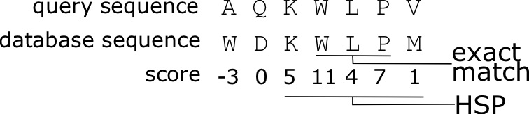
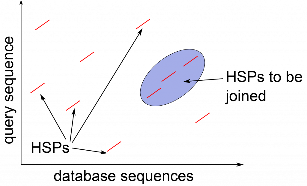
The BLAST algorithm (Basic Local Alignment Search Tool) developed by Altschul (1990) combines indexing of a database of sequences, and heuristics to approximate Smith-Waterman alignment, but is [latex]50 \times[/latex] faster. The approach of BLAST is to index a search database using [latex]K[/latex]-mers, subsequences of length [latex]K[/latex], for each of the sequences in the database. A query sequence is input to the program to search for similar sequences in the database. After low-complexity sequences are removed, all [latex]K[/latex]-mers of the query sequence are listed, and possible matches in the database are identified that would have an alignment score as good as [latex]T[/latex], a predefined score threshold. The matching [latex]K[/latex]-mers are extended into stretches of matching [latex]K[/latex]-mers, that are called High-scoring Segment Pairs (HSPs), resulting in matches that are longer than [latex]K[/latex]. Two or more of these HSPs are combined to form a longer alignment. Ultimately Smith-Waterman alignment is performed on just these strongly matching sequences, and this is what is reported.
In summary, the approach is as follows:
- Remove low0complexity regions or sequence repeats in the query sentence.
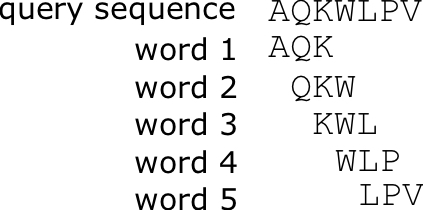
- Make [latex]K[/latex]-mer word list of the query sequence (Proteins often [latex]K[/latex] = 3)
- List the possible [latex]20^3[/latex] matching words with a scoring matrix
- Reduce the list of word matches with threshold T
- Extend the exact matches to High-scoring Segment Pairs (HSPs)
- List all HSPs and evaluate significance
- Combine two or more HSPs into a longer alignment
- Report the gapped Smith-Waterman local alignments of the query and each of the matched database sequences.
3.3 Alignment Statistics
When evaluating a BLAST score, it is important to have a statistical framework for evaluating the significance of a “BLAST hit”. Here we present such a system where we consider our score [latex]S[/latex] as a random variable. Because BLAST identifies the maximum scoring alignment, we can describe the cumulative distribution of BLAST scores with the Generalized Extreme Value (GEV) distribution:
[latex]P(S \le x) = \exp \left( - e^{-\lambda (x - u)}\right)[/latex]
The parameter [latex]u[/latex] is the location parameter of the GEV, and is expressed here in terms of the length [latex]n[/latex] of the query sequence, and the length [latex]m[/latex] of the entire database. [latex]K[/latex] here is a constant that is particular to and computed from a particular database.
[latex]u = \frac{\ln Knm}{\lambda}[/latex]
The p-value is the probability of a score greater than or equal to S due to chance, and is given by:
[latex]P(S \ge x) = 1 - \exp \left( -Knme^{-\lambda x}\right)[/latex]
This equation comes from the Poisson distribution. If we define E-value (expected number of hits at this score or greater due to chance) as:
[latex]E = Knme^{-\lambda S}[/latex]
The p-value can then be simplified as:
[latex]P(S \ge x) = 1 - e^{-E}[/latex]
After a linear transformation, the score S’ can be computed in terms of bits.
[latex]S' = \frac{\lambda S - \ln K}{\ln 2}[/latex]
The updated equation for E-value is much simpler:
[latex]E = nm \times 2^{-S'}[/latex]
3.3.1 Running BLAST from the command line
BLAST can be run on the command line pretty easily. To do this, you need a sequence, or set of sequences to align, and a database to align to. First, let’s create the database to align to. This can be created using a FASTA file of sequences. For example, if we have the FASTA file for the human genome [latex]\texttt{hg38.fa}[/latex], we can format the database with [latex]\texttt{makeblastdb}[/latex] using the following command:
$ makeblastdb -in hg38.fa -input_type fasta -title hg38 -dbtype nucl
In this command, most of the terms make sense. The input file is [latex]\texttt{hg38.fa}[/latex], the input file format is “fasta”, and the title used is [latex]\texttt{hg38}[/latex]. The last term specifies that the input data is nucleic acid sequences.
On some systems, an older version is installed using [latex]\texttt{formatdb}[/latex]. With this program, the database can be created using this command:
$ formatdb -p F -t hg38 -n hg38 -i hg38.fa
In this command, the [latex]\texttt{-p F}[/latex] command indicates that this is a nucleotide sequence, and not a protein sequence. Specifically, the [latex]\texttt{-p}[/latex] specifies protein, and the [latex]\texttt{F}[/latex] says that this is “false”, specifying that the input data is not protein. The second two commands give the database the title and name [latex]\texttt{"hg38"}[/latex]. The name specified by the [latex]\texttt{-n}[/latex] command provides a basename for the output files used in the database, and also gives a label to be used when referring to the database in BLAST. Finally, the [latex]\texttt{-I}[/latex] command specifies the input file, which is the FASTA file for the genome.
Next, we can run BLAST using the command [latex]\texttt{blastall}[/latex]. This tool allows you to run different versions of BLAST, specified by the [latex]\texttt{-p}[/latex] command. To run a nucleotide query against a nucleotide database, we use [latex]\texttt{blastn}[/latex]. The full command is as follows:
$ blastall -p blastn -i sequences.fa -d hg38 -o sequences_hg38_blast.txt
Here we specify the input sequences, the query, with the [latex]\texttt{-I}[/latex] command. Then we specify the database that we are aligning to, using the [latex]\texttt{-d}[/latex] flag, referring to the database that we just created with [latex]\texttt{formatdb}[/latex]. Finally, we specify an output file to write the results to, using the [latex]\texttt{-o}[/latex] flag.
3.4 Short Read Mapping
The growth of high-throughput sequencing has led to a parallel growth of software applications for rapidly aligning short reads. Although BLAST was designed for fast alignment, these new tools are even faster for the alignment of short sequence reads. We will discuss these methods further in Chapter 9.
3.5 Lab 4: Using BLAST on the command line
In this lab, we will learn how to run BLAST on the command line. As usual, you should create and enter a [latex]\texttt{Lab4}[/latex] directory.
3.5.1 Part 1: BLASTing to a protein database
Let’s first build a database. Please download the Swissprot database from NCBI with the following command:
$ wget ftp://ftp.ncbi.nih.gov/blast/db/FASTA/swissprot.gz
and then unzip the downloaded file with the following command:
$ gunzip swissprot.gz
Although there is no file extension, the file is a FASTA file. Let’s rename it so that we know it is a FASTA file.
$ mv swissprot swissprot.fa
Next, let’s build a database with the following command:
$ makeblastdb -in swissprot.fa -input_type fasta -title swissprot -dbtype prot
Not all of these options are required. Can you figure out which options are required by the help message printed with you run this command?
$ makeblastdb -help
Download the protein sequence infomation for human BRCA1 and create a fasta file for the sequence (https://www.ncbi.nlm.nih.gov/protein/1698399?report=fasta). Save it to a file called [latex]\texttt{brca1\_pep.fa}[/latex]. Copy the sequence, and paste it into a file after opening it with nano:
$ nano brca1_pep.fasta
To save with nano, type Ctrl-X, then type Y. Next, we can BLAST the brca1_pep.fasta file we created.
$ blastp -query brca1_pep.fasta -db swissprot.fa > brca1_swissprot
Do the top hits make sense to you? You can search NCBI Protein for some of the IDs.
$ less brca1_swissprot
What are the best hits? Do the order of the sequence hits make sense in terms of what you know of the biology?
You can also BLAST the sequence to the “non-redundant” database “nr” by pasting it to the NCBI BLAST web tool: https://blast.ncbi.nlm.nih.gov/Blast.cgi. Note that you could theoretically do this by specifying “nr” for the database, but many servers don’t have this downloaded (it’s a very big file!).
3.5.2 Biopython and BLAST (optional)
You could also analyze your blast hits using Biopython. To do this, you need to set the output format to XML with the following command.
$ blastp -query brca1_pep.fasta -db swissprot -outfmt 5 > brca1_swissprot.xml
The XML can be difficult to read, but can be parsed easily. For example, you can print the alignment for each BLAST hit in the results with something like this:
>>> from Bio.Blast import NCBIXML

>>> result_handle = open("brca1_swissprot.xml")

>>> blast_record = NCBIXML.read(result_handle)

>>> for alignment in blast_record.alignments:

...     for hsp in alignment.hsps:

...         if hsp.expect < 1e-10:

...             print('sequence:', alignment.title)

...             print('length:', alignment.length)

...             print('e value:', hsp.expect)

...             print(hsp.query)

...             print(hsp.match)

...             print(hsp.sbjct)
Variations on this method could allow one to parse the BLAST output file, and extract the alignments as well.
3.5.3 Part 2: BLASTing to a genome
UCSC provides a wealth of genomic resources. You can download the Drosphila genome version dm3 at this link: http://hgdownload.soe.ucsc.edu/goldenPath/dm3/bigZips/. Download [latex]\texttt{chromFa.tar.gz}[/latex] with the command at the terminal:
$ wget http://hgdownload.soe.ucsc.edu/goldenPath/dm3/bigZips/chromFa.tar.gz
Unzip the file with the command:
$ tar xvfz chromFa.tar.gz
Combine all the chromosome FASTA files into one genome file:
$ cat chr*fa > dm3.fa
In this case, the asterisk is used as a wild-card, that specifies all files with anything between a [latex]\texttt{"chr"}[/latex] and a [latex]\texttt{".fa"}[/latex]. You can clean up the directory by moving the [latex]\texttt{chr*fa}[/latex] files into a directory. First create the directory:
$ mkdir genome
Move the chromosome files into the directory with this command:
$ mv chr*fa genome/.
Build a blast database:
$ makeblastdb -in dm3.fa -title dm3 -dbtype nucl
Download the transcript sequence for human BRCA1 and create a FASTA file for the sequence NCBI human BRCA1 here: https://www.ncbi.nlm.nih.gov/nuccore/1147602?report=fasta.
BLAST the sequence to the genome:
$ blastn -query brca1.fa -db dm3.fa > brca1_dm3.blast
Download the RefSeq mRNA annotations [latex]\texttt{refMrna.fa.gz}[/latex] with the command at the terminal:
$ wget http://hgdownload.soe.ucsc.edu/goldenPath/dm3/bigZips/refMrna.fa.gz
gunzip the file with the command:
$ gunzip refMrna.fa.gz
Create a database for the RefSeq annotations:
$ makeblastdb -in refMrna.fa -title refMrna -dbtype nucl
BLAST the sequence to the refMrna database:
$ blastn -query brca1.fa -db refMrna.fa > brca1_refMrna.blast
Discussion questions: What is the the difference between the two results? How do you explain the difference? What is chrUextra anyway? To answer this you should look at the BLAST output with “less” in the same way you looked at other BLAST output above.
Going beyond: How does this e-value compare to BLASTing to mouse through the NCBI website? Can you find a gene in human that has a significant hit to the E. coli genome?
