Chapter 8: Proteins
Many transcripts encode proteins, which are sequences of amino acids that fold into specific structures that determine their functions. To a great extent, the sequence of the protein determines its structure, which in turn determines its function. Therefore, identifying similar protein sequences can suggest structures and functions. The field of protein bioinformatics is certainly extensive, and we will only be able to cover a small portion to introduce some concepts that may be useful.
To go from mRNA to protein, we need an open reading frame (ORF) defined by a start codon in frame with a stop codon. Typical mRNAs have many possible ORFs, with other signals, such as the Kozak sequence, determining which ORF is used. In most cases, the longest ORF is the coding DNA sequence (CDS), or the region that is actually translated. In general it is important to distinguish ORFs, which are quite common, from the CDS.
Once we have the CDS sequence, it is easy to compute the corresponding peptide sequence with Biopython, as we have seen in section 1.2.2.
8.1 Protein Alignment
Our previous discussion of alignment applies to proteins as well as nucleic acid sequences. However, with 20 amino acids, our scoring system can be updated to account for chemical similarity, and the fact that some amino acids are more likely to mutated to others.
Typically, when aligning two sequences, the assumption is that the two sequences have a common evolutionary origin, and the association between single characters in the alignment correspond to the evolutionary history of those characters. In order to optimize such an alignment, we need to define a scoring system used to compare two characters.
Let's define some probabilistic models of sequence alignments so that we can describe the scoring system with such a formalism. Much of what we will describe here was developed for protein sequences, but the formalism could be used more generally. First, let's formulate the probability of the two sequences given a random model. That is, the two sequences are just two random strings of characters that have been independently generated from a generative probabilistic model.
Consider an ungapped alignment of the sequences [latex]x[/latex] and [latex]y[/latex]:
x[1]x[2]x[3]x[4] ... x[n]

| | | | |

y[1]y[2]y[3]y[4] ... y[n]
Let's work out a scoring system for this, and then later introduce gaps.
For a random model, each of the characters [latex]x[i][/latex] and [latex]y[i][/latex] at each position [latex]i[/latex] is just randomly selected according to their frequency in the database
[latex]P(x,y|Random) = \prod_{i=1}^n p_{x[i]} p_{y[I]}[/latex]
Alternatively, if the sequences have a common ancestor, we could also define a probability [latex]q_{a,b}[/latex] as describing the frequency of occurrence of substitutions in the database between two characters [latex]a[/latex] and [latex]b[/latex].
[latex]P(x,y|Ancestor) = \prod_{i=1}^n q_{x[i],y[I]}[/latex]
If we combine our two probabilistic models, we can compute a odds ratio
[latex]\frac{P(x,y|Ancestor)}{P(x,y|Random)} = \frac{\prod_{i=1}^n q_{x[i],y[i]}}{\prod_{i=1}^n p_{x[i]} p_{y[i]}}[/latex]
and by taking a logarithm, we can define a score as a log-odds ratio, which is more convenient for our purpose because it turns the product into a sum
[latex]S = \log \left( \frac{P(x,y|Ancestor)}{P(x,y|Random)} \right) = \log \left(\frac{\prod_{i=1}^n q_{x[i],y[i]}}{\prod_{i=1}^n p_{x[i]} p_{y[i]}} \right) = \sum_{i=1}^n \log \left( \frac{q_{x[i],y[i]}}{p_{x[i]} p_{y[i]}} \right)[/latex]
The last terms give us our similarity matrix terms [latex]S_{a,b}[/latex] defined as
[latex]S_{a,b} = \log \left( \frac{q_{a,b}}{p_a p_b} \right)[/latex]
8.1.1 PAM Matrices
A Point Accepted Mutation Matrix (PAM Matrix), is was the first systematically defined matrix for scoring the similarity of peptide sequences. This scoring system was created by Margaret Dayhoff in 1978 [80]. First we define a "Mutation Matrix" [latex]M[/latex] that describes the probability of mutating from [latex]a[/latex] to [latex]b[/latex].
[latex]M_{ab} = P(a \rightarrow b)[/latex]
The Mutation matrix is time reversible, meaning
[latex]P(a)M_{ab} = P(b)M_{ba}[/latex]
Under such a time-reversible model, the observed frequency of [latex]a[/latex] mutating to [latex]b[/latex] is equal to the observed frequency of [latex]b[/latex] mutating to [latex]a[/latex]. This is a common assumption, particularly because we can't observe, and can only infer, which character is ancestral. We will see below that we can compute the most likely or most parsimonious ancestral character, but the databases that were originally used to build these scoring matrices just used alignments; hence, we can only observe substitutions.
If our database has [latex]n_a[/latex] occurrences of amino acid [latex]a[/latex], then we define our normalized frequency [latex]p_a[/latex] of that amino acid as
[latex]p_a = \frac{n_a}{N}[/latex]
where [latex]N[/latex] is the total number of amino acids in the database. Because [latex]\sum_a n_a = N[/latex], the probabilities [latex]p_a[/latex] are normalized.
We can't measure how much time has transpired between mutations in the sequences of our database. Therefore, we have to talk about how many substitutions have taken place as a percentage.
These mutation matrices are scaled such that there is [latex]1%[/latex] amino acid change:
[latex]\sum_{a=1}^{20} p_a M_{aa} = 0.99[/latex]
Therefore, this equation scales the mutation rates, and gives us restrictions on the protein alignments that we can consider in our database.
The actual PAM matrix that is used in scoring is defined as
[latex]PAM_1(a,b) = \log \left( \frac{p_a M_{a,b}}{p_a p_b} \right) = \log \left( \frac{M_{a,b}}{p_b } \right)[/latex]
To get more distant relationships, we can raise the matrix [latex]M = M^{(1)}[/latex] to a power.
[latex]M^{(n)} = \left( M^{(1)} \right)^n[/latex]
Consider [latex]M^2[/latex]:
The result of this matrix product gives the probability of mutating from [latex]a[/latex] to [latex]c[/latex] in twice the amount of time defined by the matrix [latex]M[/latex], and considering all intermediate amino acids [latex]b[/latex].
[latex]M_{ac} = \sum_{b} M_{ab} M_{bc} = \sum_b P(a \rightarrow b) P(b \rightarrow c)[/latex]
PAM matrices of a higher order, are then defined by taking the log of this higher-order power of the original PAM matrix.
[latex]PAM_n(a,b) = \log \left( \frac{p_a M^{(n)}_{a,b}}{p_a p_b} \right) = \log \left( \frac{M^{(n)}_{a,b}}{p_b } \right)[/latex]
Therefore, the larger [latex]n[/latex] is, it describes more distant homology. For example, [latex]PAM_{250}[/latex] is an option in NCBI BLAST to specify more distance relationships.
8.1.2 BLOSUM Matrices
Another very common set of protein substitution matrices is BLOSUM [81]. BLOSUM is actually a series of matrices BLOSUM-x, where they are built from alignments that are at least [latex]x\%[/latex] identical.
These alignments come from the Blocks Database , which is still available at [latex]\texttt{http://blocks.fhcrc.org}[/latex].
Consider a single column of one of these Block alignments
| Block Alignment |
|---|
| [latex]\texttt{...L...}[/latex] |
| [latex]\texttt{...L...}[/latex] |
| [latex]\texttt{...L...}[/latex] |
| [latex]\texttt{...I...}[/latex] |
| [latex]\texttt{...I...}[/latex] |
| [latex]\texttt{...V...}[/latex] |
| [latex]\texttt{...V...}[/latex] |
In this example, there are 3[latex]\texttt{L}[/latex], 2 [latex]\texttt{I}[/latex]s, and 2 [latex]\texttt{V}[/latex]s. We wish to compute the number of pairs [latex]f_{ij}[/latex] for each pair of amino acids [latex]i[/latex] and [latex]j[/latex]. When the amino acid is the same, for example [latex]f_{LL}[/latex] is the number of pairs that can be selected from [latex]n_L[/latex] items, or [latex]{ n_L \choose 2}[/latex], where [latex]n_L[/latex] is the number of occurrences of the amino acid [latex]\texttt{L}[/latex]. This expression can be expanded in terms of factorials as follows.
[latex]{ n_L \choose 2} = \frac{n_L!}{2! (n_L - 2)!}[/latex]
(8.1)
When the amino acids are different, such as [latex]f_{IL}[/latex], the value is computed as the product of the number of occurrences of each amino acid, like [latex]f_{IL} = n_L \times n_I = 3 \times 2 = 6[/latex]. To avoid double counting, we can only consider cases when latex i \le j$.
These frequencies are normalized to make a [latex]q_{ij}[/latex] matrix, with terms defined as
[latex]q_{ij} = \frac{f_{ij}}{\sum_{i=1}^{20} \sum_{j=i}^{20} f_{ij}}[/latex]
Where the second sum in the denominator just goes up to [latex]i[/latex] to count half of the symmetric matrix [latex]f_{ij}[/latex] to avoid double-counting pairs.
We can get the normalized frequencies of each animo acid from these quantities by
[latex]p_i = q_{ii} + \frac{1}{2} \sum_{j \ne i} q_{ij}[/latex]
where the [latex]1/2[/latex] term is because there is a probability of [latex]1/2[/latex] that a random amino acid selected from the pairs corresponding to the [latex]q_{ij}[/latex] pairs is [latex]i[/latex]. Next we want to compute the probability [latex]e_{ij}[/latex] of selecting the amino acids [latex]i[/latex] and [latex]j[/latex] by random.
[latex]e_{ij} = \begin{cases} p_i p_j, & \text{if } i=j \\ p_i p_j+p_j p_i = 2 p_i p_j, & \text{if } i \ne j \end{cases}[/latex]
To understand this equation, imagine selecting a pair of amino acids at random from the database. If they are the same, then the probability of that happening is just [latex]p_i p_i = p_i^2[/latex]. If they are different, then there are two ways that could be selected: first [latex]i[/latex] then [latex]j[/latex], and first [latex]j[/latex] then [latex]i[/latex]. Finally, the BLOSUM matrix would be computed as a log-likelihood ratio
[latex]S_{i,j} = \log \left( \frac{q_{ij}}{e_{ij}} \right)[/latex]
In practice, the values for the BLOSUM matrices are rounded to integers because when they were created computer memory and computation was expensive, and this required less space than storing decimals and performing floating point arithmetic.
8.1.3 Karlin and Altschul Generalization
Karlin and Altschul formulated a generalized scoring matrix that is similar to both PAM matrices and BLOSUM matrices, defined as
[latex]S_{i,j} = \left( \frac{1}{\lambda} \right) \ln \left( \frac{q_{i,j}}{p_i p_j} \right)[/latex]
where [latex]\lambda[/latex] is a positive parameter that scales the matrix [82].
8.1.4 Biopython and Substitution Matrices
We can access values of a given substitution matrix using Biopython and the module [latex]\texttt{Bio.SubsMat}[/latex]. For example, the most commonly used substitution matrix and the default for NCBI protein BLAST is BLOSUM62. We can print the values of the matrix or access a particular term by the following
>>> from Bio.SubsMat import MatrixInfo

>>> S = MatrixInfo.blosum62

>>> S['Q','Q']

5

>>> S['W','Q']

-2
If you play around with this matrix (actually it is a dictionary that takes a pair of characters as keys) you will realize that some pairs are stored, but others are not and return errors when one tries to access them. For example, [latex]\texttt{S['W','Q']}[/latex] is stored, but not [latex]\texttt{S['Q','W']}[/latex]. To get around this, an additional function can be created:
>>> def getScore(a,b,S):

...     if (a,b) not in S:

...         return S[b,a]

...     return S[a,b]

...

>>> getScore('Q','W',S)

-2
8.2 Functional Annotation of Proteins
Computational methods can be used to infer protein function when a new protein is identified, but even if the inference is very strong, experiments still need to be done to validate the prediction. That said, there are many ways in which a hypothesis about protein function can be inferred, including sequence homology, sequence motifs such as "domains", which could be considered a type of homology, structure-based function prediction, genomic co-location (gene clusters), gene expression data, in particular co-expression.
8.2.1 Protein Evolution and Homology
The first method that one might use to infer protein function is by sequence homology. Frequently, the more fundamental molecular functions of proteins are very well conserved. There are a number of mechanisms of protein evolution that one must consider when evaluating protein homology.
In DNA replication, there are often errors that cause major changes in proteins, which can be highly disruptive to the function of the protein, but perhaps in some cases may confer new function. First, is the event of gene fusion, where two genes may be merged into one gene, combining different functional regions from the two ancestral genes. For example, a gene encoding a protein with a DNA-binding domain could fuse with a gene encoding a protein with a protein-binding domain, producing a new gene encoding a protein with both domains. In many cases, a gene fusion event is caused by a chromosomal translocation event, but such translocations can also cause other mutations in genes, such as loss of a portion of a gene. In addition, regions of chromosomes can be inverted during replication, resulting in gene fusions or deletions of portions of genes. Along the same lines, a chromosomal deletion, where a portion of a chromosome is deleted during DNA replication, can also lead to gene fusion events or loss of a portion of a gene.
Gene duplication events can happen as part of a chromosomal duplication, or as part of a local duplication. When this happens, multiple copies of a gene can be created. The two copies of the gene could be beneficial in some cases, or harmful in others. In these cases, one of the copies can be possibly silenced. When both copies remain, one of the copies can undergo less selective pressure, because the bulk of the work is carried out by one of them. In this case, the other copy can accumulate mutations over time, which could result in new function or a specialized function. This process where one copy accumulates mutations and ultimately carries out a specialized role is often called sub-functionalization of the protein [83, 84].
8.2.2 Protein Domains
A protein domain is a conserved part of the protein that has a distinct structure and function. Often domains occur as highly conserved blocks of conservation that can be clearly observed in a sequence alignment. Often distantly related genes have domains conserved beyond the rest of the gene. Domains also will fold and evolve independently of the rest of the protein, resulting in increased conservation over the domain region. The idea of a protein domain was introduced by Wetlaufer in 1973 through observing common stable units in X-ray crystallography studies [85].
A protein domain can be understood as similar to a motif, although some databases have more complex representations when necessary to describe a more complex pattern. To identify protein domains, one needs a sufficiently diverged set of proteins in order to accumulate enough mutations outside the domain so that the domain itself can be identified. However, with a set of proteins that is too diverged, once could even lose the conservation of the domain.
Many databases of protein domains exist, including Pfam, PANTHER, PROSITE, and Interpro.
Pfam Database
Pfam is a database of proteins, protein families [86], and domains, and is available at http://pfam.sanger.ac.uk. Pfam domains are a commonly used annotation of protein domains that are relatively easy to use.
For example, one can use the program HMMer (pronounced "hammer") to scan Pfam domains downloaded as an hmm file. The command would be something like this:
$ hmmscan --domtblout domainTable.txt Pfam-A.hmm proteins.fasta
To produce a table similar to a BLAST output with locations of matches, e-values, and p-values.
8.3 Secondary Structure prediction
To get a full view of a protein's structure, we'll need a way to compute its tertiary structure, which is extremely difficult. In practice, we have to rely on experimental evidence such as X-ray crystallographic studies or NMR structures. Some studies will use a known structure of a protein and apply it to a homologous protein. Secondary structure for proteins can be computed, however, with reasonable accuracy. The secondary structure of a protein is a list of the positions corresponding to alpha helices and beta strands.
The software [latex]\texttt{jnet}[/latex] can predict secondary structural features and provide a confidence score for each position [87]. For example, the program [latex]\texttt{jnet}[/latex] can be run on the command line with a command like:
$ jnet -p human_catalase.fasta
to produce an output file indicating the locations of these regions:
Length = 527 Homologues = 1

RES : MADSRDPASDQMQHWKEQRAAQKADVLTTGAGNPVGDKLNVITVGPRGPLLVQDVVFTDEMAHFD

ALIGN : ---------HHHHHHHHHHHHHH--EEE---------EEEEEEE-----EEEEEEEE-----H--

CONF : 88888887525778889988874122440687775752678883477752575455201000013

FINAL : ---------HHHHHHHHHHHHHH--EEE---------EEEEEEE-----EEEEEEEE--------
where the [latex]\texttt{CONF}[/latex] value is the confidence, a number from [latex]0[/latex] to [latex]9[/latex], that indicates the quality of the prediction. In this representation, the [latex]\texttt{H}s[/latex] represent alpha helices, and the [latex]\texttt{E}s[/latex] indicate beta-strands. Here we have run the program with one protein sequence, but it could be run with multiple sequences for greater accuracy.
8.4 Gene Ontology
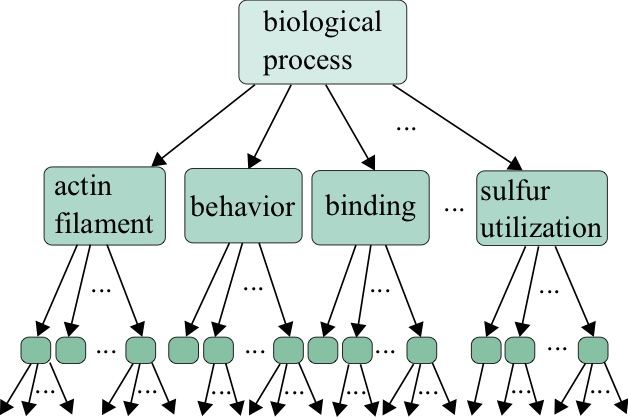
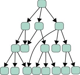
Gene Ontology (GO) is a database of controlled vocabulary terms that describe gene/protein function [88]. A valuable web resource for GO terms and related data is available at their website (http://geneontology.org). These terms form a hierarchy, where certain higher-level terms "contain" the lower-level terms in conceptual scope.
There are many levels of evidence for the assignment of a GO term, indicated by "evidence codes", given by a symbol of a few letters. For example, [latex]\texttt{EXP}[/latex] indicates that the term was "Inferred by experiment" Others such as [latex]\texttt{TAS}[/latex] for "traceable author statement" indicate that there is a statement in a publication making the claim of the association.
| Evidence Code | Meaning |
|---|---|
| TAS | Traceable Author Statement |
| EXP | Inferred from Experiment |
| IDA | Inferred from Direct assay |
| IPI | Inferred from Physical Interaction |
| IMP | Inferred from Mutant Phenotype |
| IGI | Inferred from Genetic Interaction |
| IEP | Inferred from Expression Pattern |
| ISS | Inferred from Sequence or Structural Similarity |
| ISO | Inferred from Sequence Othology |
8.4.1 Multiple hypothesis testing
Frequently when performing a study on the effect of a mutation or other treatment, one looks at the GO terms of the genes that are significantly differentially expressed due to the experimental condition compared to a control. One evaluates whether the enrichment of a particular GO term in the data exceeds that of the expected rate of this term occurring in randomly sampled gene sets of the same size. This significance is typically computed from a p-value describing the enrichment.
However, in doing so, one needs to perform a multiple test correction, to account for the fact that many hypotheses were tested. For example, if you found a one-in-a-million event after examining one million events, you might not be surprised. The simplest multiple-test correction is the Bonferroni correction [89], where when testing [latex]N[/latex] hypotheses, we need to test for significance at level [latex]\alpha[/latex] by examples satisfying the relationship:
[latex]p N \le \alpha[/latex]
(8.2)
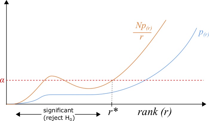
Another method is the Benjamini-Hochberg procedure, which is a little bit more complex [90]. To do this procedure, one needs to sort the list of p-values [latex]{p_1,p_2,...,p_N}[/latex] in ascending order such that [latex]p_{(1)} \le p_{(2)} \le ... \le p_{(N)}[/latex] such that the subscript given by [latex]p_{(r)}[/latex] indicates the p-value with rank [latex]r[/latex]. This procedure gives us a list of significant hypotheses with a rate of false-discovery defined by the imposed [latex]FDR[/latex], a number between [latex]0[/latex] and [latex]1[/latex]. After the sorting, all p-values with a rank [latex]r[/latex] less than the maximum rank [latex]r^*[/latex] such that:
[latex]\frac{p_{(r^*)} N}{r^*} \le FDR,[/latex]
(8.3)
where [latex]FDR[/latex] defines the false discovery rate, are deemed significant.
8.5 Lab 9: Proteins
In this lab, we learn some methods for predicting properties of protein sequences, such as domains and secondary structure.
8.5.1 Scanning for domains
First, let's look at protein domains from Pfam. First, we'll need to download a domain file from Pfam with the following command:
$ wget ftp://ftp.ebi.ac.uk/pub/databases/Pfam/current_release/Pfam-A.hmm.gz
This file contains a set of HMM models for protein domains defined for the Pfam database. To use this file, we must first unzip the file with gunzip.
$ gunzip Pfam-A.hmm.gz
This will produce the unzipped file [latex]\texttt{Pfam-A.hmm}[/latex], which can be used to scan for these domains using the HMMer software program hmmscan as part of the HMMer package. However, we still need to index this [latex]\texttt{.hmm}[/latex] domain file. This can be done with the HMMer software.
$ hmmpress Pfam-A.hmm
As we have seen in this course, there are many ways to download a protein sequence. Since we will work on protein secondary structure prediction, let's consider downloading something from PDB, the Protein Databank.
The PDZ domain is a structural domain involved in signaling in many organisms ranging from bacteria to animals. The structure consists of roughly 5 beta-strands and 2 alpha-helices, as demonstrated by this image of the tertiary structure [91].
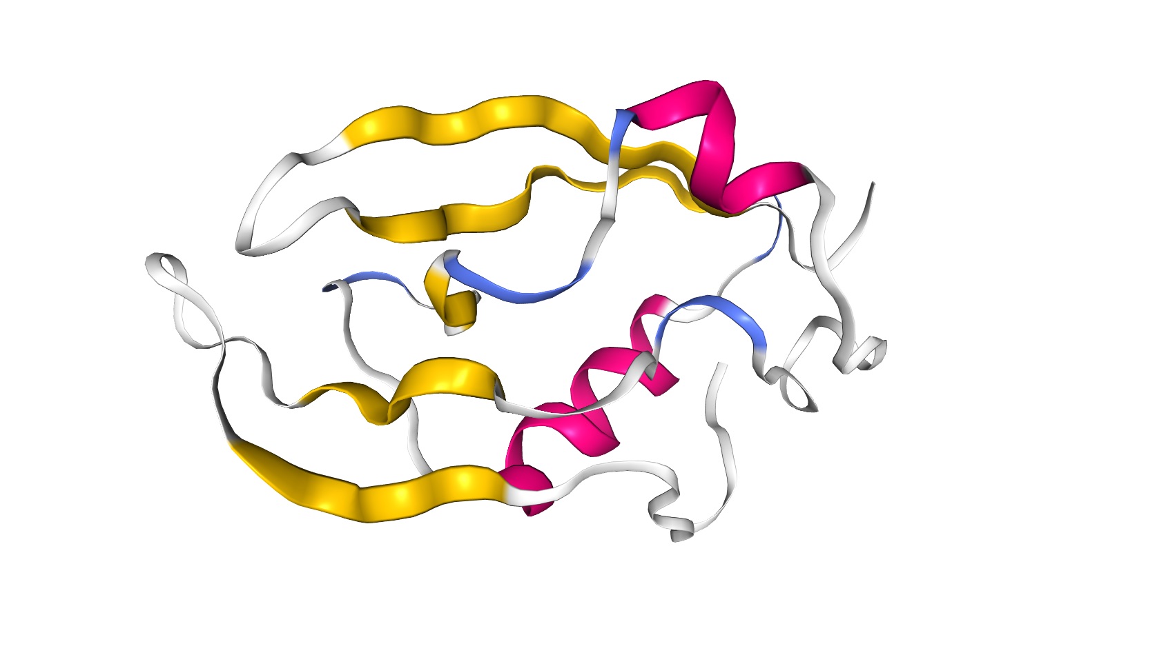
You can see more detail on this structure at PDB (http://www.rcsb.org/3d-view/2NB4/1). One useful piece of data in this database entry is the secondary structure information found at the PDB database here: http://www.rcsb.org/pdb/explore/remediatedSequence.do?structureId=2NB4 (inactive link as of 05/28/2021).
The sequence can be obtained in the upper-right hand corner of the PDB database page under "Download Files" and then under "FASTA sequence". Here is the PDZ domain sequence:
>2NB4

PLTRPYLGFRVAVGRDSSGCTTLSIQEVTQTYTGSNG

GADLMGPAFAAGLRVGDQLVRFAGYTVTELAAFNTVV

ARHVRPSASIPVVFSRDGVVMSATIVVGELE
Download the FASTA file here PDZ sequences and compute a multiple sequence alignment for the sequences to see if it improves the domain identification.
Now we can save this sequence to a file called [latex]\texttt{pdz.fasta}[/latex]. We can then run [latex]\texttt{hmmscan}[/latex] to see if there are any domains in this sequence:
$ hmmscan --domtblout domains_2NB4.txt Pfam-A.hmm pdz.fasta
Does this output make sense? you can view it with the following command, using "less -S" to turn off word-wrapping.
$ less -S domains_2NB4.txt
The first few columns define which domain was found. As expected the only domains are PDZ. What is unexpected, perhaps, is the positions of the two Pfam domains pertaining to PDZ (defined by the "ali coord" entry and "from" and "to" columns.) don't always start at the same position, suggesting that to some degree the boundaries are a bit "fuzzy" at times.
Also, note that another column provides the e-value, which is interpreted similarly to BLAST, as the expected number of occurrences of this domain by chance
The secondary structure of the protein can be computed with the following command:
$ jnet -p pdz.fasta
This produces a file format that gives the sequence and a letter designation for whether the region is an alpha-helix, designated by an "H", or a beta-strand, designated by an "E". How closely does the predicted structure correspond to the true structure seen here: https://www.rcsb.org/pdb/explore/remediatedSequence.do?structureId=2NB4 (inactive link as of 05/28/2021)?
You can run this program on an alignment, but you need to remove gaps from the multiple sequence alignment. To do this, first compute an alignment. I used the PDZ file above
$ clustalw2 -infile=PDZ_sequences.fasta -type=Protein -outfile=PDZ_sequences.aln
Next, you need to convert to FASTA alignment format and remove gaps. You can covert to FASTA using AlignIO (see Lab 5, section 4.4), but this will not remove gaps. To remove gaps, very industrious students might try to write a python script to do this. Note that you need to remove gaps a column of the alignment. Meaning, if one sequence has a gap, that specific position of the alignment would be removed for all sequences. Alternatively, you an use the program [latex]\texttt{trimal}[/latex] to do this. You can remove the gaps and convert to FASTA in one step:
$ trimal -in PDZ_sequences.aln -fasta -nogaps > PDZ_sequences.fa
Next, you can run [latex]\texttt{jnet}[/latex] on the resulting alignment:
$ jnet -p PDZ_sequences.fa
The problem here is whether or not the alignment with gaps removed is informative. If your sequences are too far away, a lot of gaps could be removed, rendering the positions of the resulting gap-free alignment different from the original sequences.
