4.1 Multiple Sequence Alignment

A multiple sequence alignment is an alignment of more than 2 sequences. It turns out that this makes the problem of alignment much more complicated, and much more computationally expensive. Dynamic programming algorithm such as Smith-Waterman can be extended to higher dimensions, but at a significant computing cost. Therefore, numerous methods have been developed to make this task faster.

4.1.1 MSA Methods

There have been numerous methods developed for computing MSAs do make them more computationally feasible.

Dynamic Programming

Despite the computational cost of MSA by Dynamic Programming, there have been approaches to compute multiple sequence alignments using these approaches [24,25]. The programs MSA [25] and MULTALIN [26] use dynamic programming. This process takes [latex]O(L^N)[/latex] computations for aligning [latex]N[/latex] sequences of length [latex]L[/latex]. The Carrillo-Lipman Algorithm uses pairwise alignments to constrain the search space. By only considering regions of the multi-sequence alignment space that are within a score threshold for each pair of sequences, the [latex]L^N[/latex] search space can be reduced.

Progressive alignments

Progressive alignments begin by performing pairwise alignments, by aligning each pair of sequences. Then it combines each pair and integrates them into a multiple sequence alignment. The different methods differ in their strategy to combine them into an overall multiple sequence alignment. Most of these methods are “greedy”, in that they combine the most similar pairs first, and proceed by fitting the less similar pairs into the MSA. Some programs that could be considered progressive alignment include T-Coffee [27], ClustalW and its variants [28], and PSAlign [29].

Iterative Alignment

Iterative Alignment is another approach that improves upon the progressive alignment because it starts with a progressive alignment and then iterates to incrementally improve the alignment with each iteration. Some programs that could be considered iterative alignment include CHAOS/DIALIGN [30], and MUSCLE [31].

Full Genome Alignments

Specialized multiple sequence alignment approaches have been developed for aligning complete genomes, to overcome the challenges associated with aligning such long sequences. Some programs that align full genomes include MLAGAN (using LAGAN) [32], MULTIZ (using BLASTZ) [33], LASTZ [34], MUSCLE [31], and MUMmer [35, 36].

4.1.2 MSA File Formats

There are several file formats that are specifically designed for multiple sequence alignment. These approaches can differ in their readability by a human, or are designed for storing large sequence alignments.

Multi-FASTA Format

Probably the simplest multiple sequence alignment format is the Multi-FASTA format (MFA), which is essentially like a FASTA file, such that each sequence provides the alignment sequence (with gaps) for a given species. The deflines can in some cases only contain information about the species, and the file name, for example, could contain information about what sequence is being described by the file. For short sequences the mfa can be human readable, but for very long sequences it can become difficult to read. Here is an example [latex]\texttt{.mfa}[/latex] file that shows the alignment of a small (28aa) Drosophila melanogaster peptide called Sarcolamban (isoform C) with its best hits to [latex]\texttt{nr}[/latex].

D.melanogaster
--------------------------------------------------
--------------------------------MSEARNLFTTFGILAILL
FFLYLIYA---------------------VL---------------
>D.sechellia
--------------------------------------------------
--------------------------------MSEARNLFTTFGILAILL
FFLYLIYAPAAKSESIKMNEAKSLFTTFLILAFLLFLLYAFYEAAF
>D.pseudoobscura
MSEAKNLMTTFGILAFLLFCLYLIYASNNSKRWPTFCGEAEFRSENSESQ
LLRAFSYERLEQCPNKKYPPKQPTTTTTKPIKMNEARSLFTTFLILAFLL
FLLYAFYEA--------------------AF---------------
>D.busckii
--------------------------------------------------
--------------------------------MNEAKSLVTTFLILAFLL
FLLYAFYEA--------------------AF---------------


Clustal

The Clustal format was developed for the program [latex]\texttt{clustal}[/latex] [37], but has been widely used by many other programs [28, 38]. This file format is intended to be fairly human readable in that it expresses only a fixed length of the alignment in each section, or block. Here is what the Clustal format looks like for the same Sarcolamban example:

CLUSTAL W (1.83) multiple sequence alignment

D.melanogaster    ------------------------------------------------------------
D.sechellia       ------------------------------------------------------------
D.pseudoobscura   MSEAKNLMTTFGILAFLLFCLYLIYASNNSKRWPTFCGEAEFRSENSESQLLRAFSYERL
D.busckii         ------------------------------------------------------------


D.melanogaster    ----------------------MSEARNLFTTFGILAILLFFLYLIYA------------
D.sechellia       ----------------------MSEARNLFTTFGILAILLFFLYLIYAPAAKSESIKMNE
D.pseudoobscura   EQCPNKKYPPKQPTTTTTKPIKMNEARSLFTTFLILAFLLFLLYAFYEA-----------
D.busckii         ----------------------MNEAKSLVTTFLILAFLLFLLYAFYEA-----------
                                        *.**:.*.*** ***:***:** :*


D.melanogaster    ---------VL---------------
D.sechellia       AKSLFTTFLILAFLLFLLYAFYEAAF
D.pseudoobscura   ---------AF---------------
D.busckii         ---------AF---------------
                            :

The clustal format has the following requirements, which can make it difficult to create one manually. First, the first line in the file must start with the words “[latex]\texttt{CLUSTAL W}[/latex]” or “[latex]\texttt{CLUSTALW}[/latex]“. Other information in the first line is ignored, but can contain information about the version of [latex]\texttt{CLUSTAL W}[/latex] that was used to create it. Next, there must be one or more empty lines before the actual sequence data begins. The rest of the file consists of one or more blocks of sequence data. Each block consists of one line for each sequence in the alignment. Each line consists of the sequence name, defline, or identifier, some amount white space, then up to 60 sequence symbols such as characters or gaps. Optionally, the line can be followed by white space followed by a cumulative count of residues for the sequences. The amount of white space between the identifier and the sequences is usually chosen so that the sequence data is aligned within the sequence block. After the sequence lines, there can be a line showing the degree of conservation for the columns of the alignment in this block. Finally, all this can be followed by some amount of empty lines.

MAF

The Multiple Alignment Format (MAF) can be a useful format for storing multiple sequence alignment information. It is often used to store full-genome alignments at the UCSC Genome Bioinformatics site. The file begins with a header beginning with [latex]\texttt{##maf}[/latex] and information about the version and scoring system. The rest of the file consists of alignment blocks. Alignment blocks start with a line that begins with the letter [latex]\texttt{a}[/latex] and a score for the alignment block. Each subsequent line begins with either an [latex]\texttt{s}[/latex], a [latex]\texttt{i}[/latex], or an [latex]\texttt{e}[/latex] indicating what kind of line it is. The lines beginning with [latex]\texttt{s}[/latex] contain sequence information. Lines that begin with [latex]\texttt{i}[/latex] typically follow each [latex]\texttt{s}[/latex]-line, and contain information about what is occurring before and after the sequences in this alignment block for the species considered in the line. Lines beginning with [latex]\texttt{e}[/latex] contain information about empty parts of the alignment block, for species that do not have sequences aligning to this block. For example, the following is a portion of the alignment of the Human Genome (GRCh38/hg38) [latex]\texttt{chr22}[/latex] with 99 vertebrates.

##maf version=1 scoring=roast.v3.3
a score=49441.000000
s hg38.chr22 10514742 28 + 50818468 acagaatggattattggaacagaataga
s panTro4.chrUn_GL393523 96163 28 + 405060 agacaatggattagtggaacagaagaga
i panTro4.chrUn_GL393523 C 0 C 0
s ponAbe2.chrUn 66608224 28 - 72422247 aaagaatggattagtggaacagaataga
i ponAbe2.chrUn C 0 C 0
s nomLeu3.chr6 67506008 28 - 121039945 acagaatagattagtggaacagaataga
i nomLeu3.chr6 C 0 C 0
s rheMac3.chr7 24251349 14 + 170124641 --------------tggaacagaataga
i rheMac3.chr7 C 0 C 0
s macFas5.chr7 24018429 14 + 171882078 --------------tggaacagaataga
i macFas5.chr7 C 0 C 0
s chlSab2.chr26 21952261 14 - 58131712 --------------tggaacagaataga
i chlSab2.chr26 C 0 C 0
s calJac3.chr10 24187336 28 + 132174527 acagaatagaccagtggatcagaataga
i calJac3.chr10 C 0 C 0
s saiBol1.JH378136 10582894 28 - 21366645 acataatagactagtggatcagaataga
i saiBol1.JH378136 C 0 C 0
s eptFus1.JH977629 13032669 12 + 23049436 ----------------gaacaaagcaga
i eptFus1.JH977629 C 0 C 0
e odoRosDiv1.KB229735 169922 2861 + 556676 I
e felCat8.chrB3 91175386 3552 - 148068395 I
e otoGar3.GL873530 132194 0 + 36342412 C
e speTri2.JH393281 9424515 97 + 41493964 I
e myoLuc2.GL429790 1333875 0 - 11218282 C
e myoDav1.KB110799 133834 0 + 1195772 C
e pteAle1.KB031042 11269154 1770 - 35143243 I
e musFur1.GL896926 13230044 2877 + 15480060 I
e canFam3.chr30 13413941 3281 + 40214260 I
e cerSim1.JH767728 28819459 183 + 61284144 I
e equCab2.chr1 43185635 316 - 185838109 I
e orcOrc1.KB316861 20719851 245 - 22150888 I
e camFer1.KB017752 865624 507 + 1978457 I

The [latex]\texttt{s}[/latex] lines contain 5 fields after the [latex]\texttt{s}[/latex] at the beginning of the line. First, the source of the column usually consists of a genome assembly version, and chromosome name separated by a dot “.”. Next is the start position of the sequence in that assembly/chromosome. This is followed by the size of the sequence from the species, which may of course vary from species to species. The next field is a strand, with “+” or “-“, indicating what strand from the species’ chromosome the sequence was taken from. The next field is the size of the source, which is typically the length of the chromosome in basepairs from which the sequence was extracted. Lastly, the sequence itself is included in the alignment block.

4.2 Phylogenetic Trees

A phylogenetic tree is a representation of the evolutionary history of a character or sequence. Branching points on the tree typically represent gene duplication events or speciation events. We try to infer the evolutionary history of a sequence by computing an optimal phylogenetic tree that is consistent with the extant sequences or species that we observe.

4.2.1 Representing a Phylogenetic Tree

A phylogenetic tree is often a “binary tree” where each branch point goes from one to two branches. The junction points where the branching takes place are called “internal nodes”. One way of representing a tree is with nested parentheses corresponding to branching. Consider the following example

((A,B),(C,D));


where the two characters [latex]\texttt{A}[/latex] and [latex]\texttt{B}[/latex] are grouped together, and the characters [latex]\texttt{C}[/latex] and [latex]\texttt{D}[/latex] are grouped. The semi-colon at the end is needed to make this tree in proper “newick” tree format. One of the fastest ways to draw a tree on the command line is the “ASCII tree”, which we can draw by using the function [latex]\texttt{Phylo.draw_ascii()}[/latex]. To use this, we’ll need to save our tree to a text file that we can read in. We could read the tree as just text into the python terminal (creating a string), but that would require loading an additional module [latex]\texttt{cStringIO}[/latex] to use the function [latex]\texttt{StringIO}[/latex]. Therefore, it might be just as easy to save it to a text file called [latex]\texttt{tree.txt}[/latex] that we can read in. Putting this together, we can draw the tree with the following commands:

>>> from Bio import Phylo
>>> tree = Phylo.read("tree.txt","newick")
>>> Phylo.draw_ascii(tree)
                                      ___________________________________ A
  ___________________________________|
 |                                   |___________________________________ B
_|
 |                                    ___________________________________ C
 |___________________________________|
                                     |___________________________________ D


This particular tree has all the characters at the same level, and does not include any distance or “branch length” information. Using real biological sequences, we can compute the distances along each brach to get a more informative tree. For example, we can download 18S rRNA sequences from NCBI Nucleotide. Using clustalw, we can compute a multiple sequence alignment, and produce a phylogenetic tree. In this case, the command

$ clustalw -infile=18S_rRNA.fa -type=DNA -outfile=18S_rRNA.aln

will produce the output file [latex]\texttt{18S_rRNA.dnd}[/latex], which is a tree in newick tree format. The file contains the following information

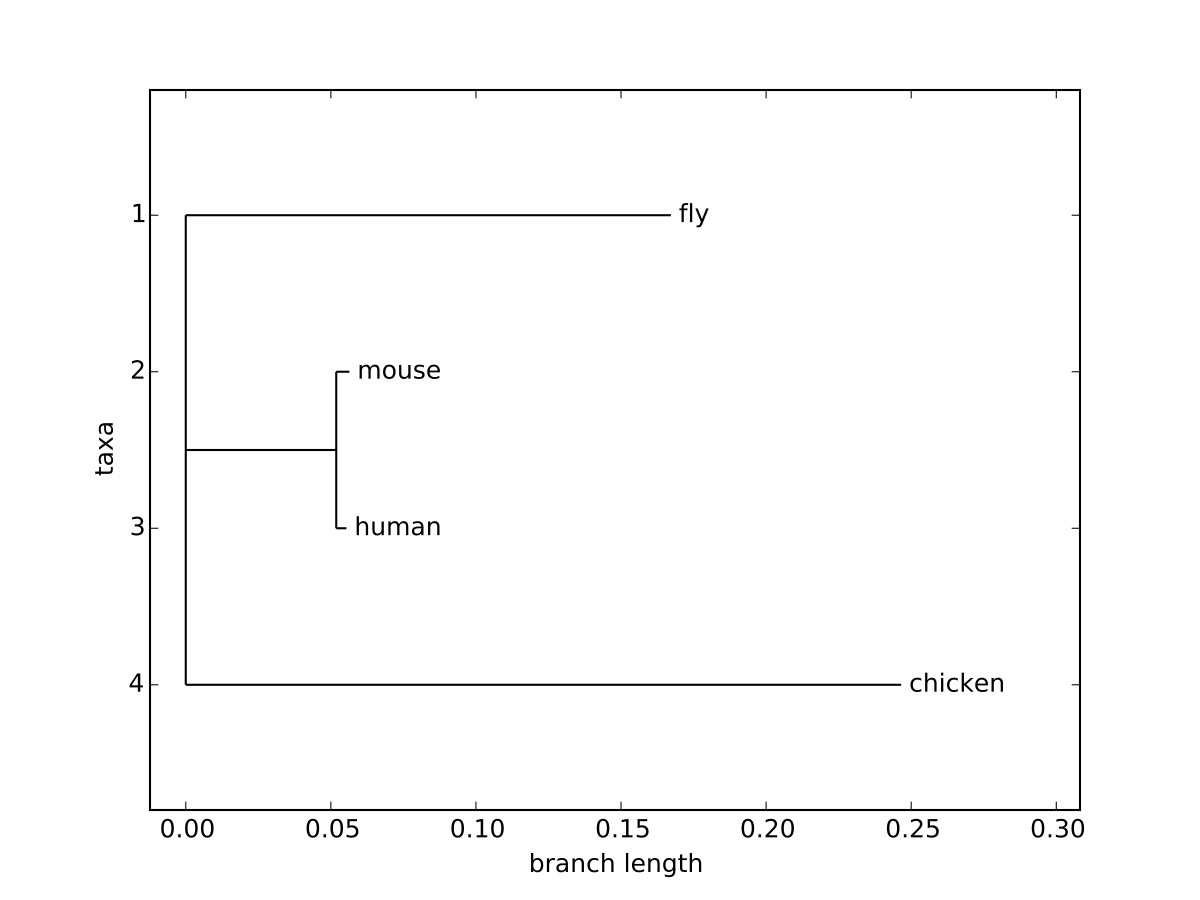
(fly:0.16718,(mouse:0.00452,human:0.00351):0.05186,chicken:0.24654);

You’ll note, this is the same format as the simple example above, but rather than a simple label for each character/sequence, there is a label and a numerical value, corresponding to the brach length, separated by a colon. In addition, each of the parentheses are followed by a colon and a numerical value. In each case, the value of the branch length corresponds to the substitutions per site required to change one sequence to another, a common unit of distance used in phylogenetic trees. This value also corresponds to the length of the branch when drawing the tree. The command to draw a tree image is simply [latex]\texttt{Phylo.draw}[/latex], which will allow the user to save the image.

>>> from Bio import Phylo
>>> tree = Phylo.read('18S_rRNA.dnd','newick')
>>> Phylo.draw(tree)

The resulting image can be seen in Figure 4.1, and visually demonstrates the branch lengths corresponding to the distance between individual sequences. The x-axis in the representation corresponds to this distance, but the y-axis only separates taxa, and the distance along the y-axis does not add to the evolutionary distance between sequences.

4.2.2 Pairwise Distances

Phylogenetic trees are often computed as binary trees with branch lengths that optimally match the pair-wise distances between species. In order to compute a phylogenetic tree, we need a way of defining this distance. One strategy developed by Feng and Doolittle is to compute a distance from the alignment scores computed from pair-wise alignments. The distance is defined in terms of an “effective”, or normalized, alignment score for each pair of species. This distance is defined as


[latex]D_{ij} = - \ln S_{eff}(i,j)[/latex]

so that pairs of sequences [latex](i,j)[/latex] that have high scores will have a small distance between them. The effective score [latex]S_{eff}(i,j)[/latex] is defined as

[latex]S_{eff}(i,j) = \frac{S_{real}(i,j) - S_{rand}(i,j)}{S_{iden}(i,j) - S_{rand}(i,j)} \times 100[/latex]

Where in this expression, [latex]S_{real}(i,j)[/latex] is the observed pairwise similarity between sequences from species [latex]i[/latex] and [latex]j[/latex]. The value [latex]S_{iden}(i,j)[/latex] is the average of the two scores when you align species [latex]i[/latex] and [latex]j[/latex] to themselves, which represents the score corresponding to aligning “identical” sequences, the maximum possible score one could get. [latex]S_{rand}(i,j)[/latex] is the average pairwise similarity between randomized, or shuffled, versions of the sequences from species [latex]i[/latex] and [latex]j[/latex]. After this normalization, the score [latex]S_{eff}(i,j)[/latex] ranges from 0 to 100.

4.3 Models of mutations

Evolution is a multi-faceted process. There are many forces involved in molecular evolution. The process of mutation is a major force in evolution. Mutation can happen when mistakes are made in DNA replication, just because the DNA replication machinery isn’t 100% perfect. Other sources of mutation are exposure to radiation, such as UV radiation, certain chemicals can induce mutations, and viruses can induce mutations of the DNA (as well as insert genetic material). Recombination is a genetic exchange between chromosomes or regions within a chromosome. During meiosis, genes and genomic DNA are shuffled between parent chromosomes. Genetic drift is a stochastic process of changing allele frequencies over time due to random sampling of organisms. Finally, natural selection is the process where differences in phenotype can affect survival and reproduction rates of different individuals.

4.3.1 Genetic Drift

Because genetic drift is a stochastic process, it can be modeled as a “rate”. The rate of nucleotide substitutions [latex]r[/latex] can be expressed as

[latex]r = \frac{\mu}{2T}[/latex]

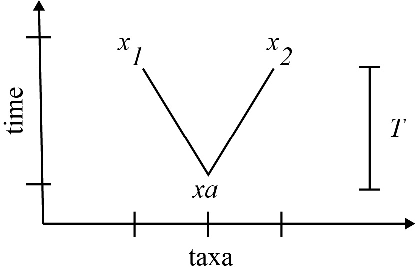
where [latex]\mu[/latex] is the substitutions per site across the genome, and [latex]T[/latex] is the time of divergence of the two (extant) species to their common ancestor. The factor of two can be understood by the fact that it takes a total of [latex]2T[/latex] to go from [latex]x_1[/latex] to [latex]x_2[/latex], stopping at [latex]x_a[/latex] along the way. The mutations that occur over time separating [latex]x_1[/latex] and [latex]x_2[/latex] can be viewed as distributed over a time [latex]2T[/latex].

In most organisms, the rate is observed to be about [latex]10^{-9}[/latex] to [latex]10^{-8}[/latex] mutations per generation. Some viruses have higher mutation rates [latex]10^{-6}[/latex] mutations per generation. The generation times of different species can also affect the nucleotide substitution rate [latex]r[/latex]. Organisms with shorter generation times have more opportunities for meiosis per unit time.

When mutation rates are evaluated within a gene, positional dependence in nucleotide evolution is observed. Because of the degeneracy in the genetic code, the third position of most codons has a higher substitution rate. Some regions of proteins are conserved domains, hence the corresponding regions of the gene have lower mutation rates compared to other parts of the gene. Other genes such as immunoglobulins have very high mutation rates and are considered to be “hypervariable”.

Noncoding RNAs have functional constraints to preserver hairpins, and may have sequence evolution that preserves base pairing through compensatory changes on the paired nucleotide. The result is that many noncoding RNAs such as tRNAs have very conserved structure, but vary at the sequence level.

4.3.2 Substitution Models

The branches of phylogenetic trees can often represent the the expected number of substitutions per site. That is, the distance along the branches of the phylogenetic tree from the ancestor to the extant species correspond to the expected number of substitutions per site in the time it takes to evolve from the ancestor to the extant species.

A substitution model describes the process of substitution from one set of characters to another through mutation. These models are often neutral, in the sense that selection is not considered, and the characters mutate in an unconstrained way. Furthermore, these models are typically considered to be independent from position to position.

Substitution models typically are described by a rate matrix [latex]Q[/latex] with terms [latex]Q_{ab}[/latex] that describe mutating from character [latex]a[/latex] to [latex]b[/latex] for terms where [latex]a \ne b[/latex]. The diagonal terms of the matrix are defined so that the sum of the rows are zero, so that

 [latex]Q_{aa} = -\sum_{b \ne a} Q_{ab}[/latex]

(4.1)

In general, the matrix [latex]Q[/latex] can be defined as:

[latex]Q = \begin{pmatrix} * & Q_{AC} & Q_{AG} & Q_{AT} \\ Q_{CA} & * & Q_{CG} & Q_{CT} \\ Q_{GA} & Q_{GC} & * & Q_{GT} \\ Q_{TA} & Q_{TC} & Q_{TG} & * \end{pmatrix}[/latex]

(4.2)

where the diagonal terms are defined such that it is consistent with Equation 4.1. The rate matrix is associated with a probability matrix [latex]P(t)[/latex], which describes the probability of observing the mutation from [latex]a[/latex] to [latex]b[/latex] in a time [latex]t[/latex] by the terms [latex]P_{ab}(t)[/latex]. We want these probabilities to be multiplicative, meaning that [latex]P(t_1)P(t_2) = P(t_1+t_2)[/latex]. The mutations associated with amounts of time [latex]t_1[/latex] and [latex]t_2[/latex] applied successively can be understood as the same as the mutations associated with [latex]t_1 + t_2[/latex]. Furthermore, the derivative of the equation can be expressed as

[latex]P'(t) = P(t)Q[/latex]

(4.3)

The solution to this equation is the exponential function. The rate matrix itself can be exponentiated to compute the probability of a particular mutation in an amount of time [latex]t[/latex], which can be computed using the Taylor series for the exponential function.

[latex]P(t) = e^{Qt} = \sum_{n=0}^{\infty} Q^n \frac{t^n}{n!}[/latex]

(4.4)

Each such model also assumes an equilibrium frequencies [latex]\pi[/latex], which describe the probability of each nucleotide after the system has reached equilibrium.

4.3.3 Jukes-Cantor 1969 (JC69)

The simplest substitution model was proposed by Jukes and Cantor (JC69), and describes equal rates of evolution between all nucleotides [39]. The JC69 model defines a constant mutation rate [latex]\mu[/latex], and equilibrium frequencies such that [latex]\pi_A = \pi_C = \pi_G = \pi_T = \frac{1}{4}[/latex]. The equilibrium frequencies describe the frequencies of each nucleotide that result after the system has evolved under this model for a “very long time”. The rate matrix for the Jukes-Cantor model is then given by:

[latex]{Q = \begin{pmatrix} -\frac{3}{4}\mu & \frac{\mu}{4} & \frac{\mu}{4} & \frac{\mu}{4} \\ \frac{\mu}{4} & -\frac{3}{4}\mu & \frac{\mu}{4} & \frac{\mu}{4} \\ \frac{\mu}{4} & \frac{\mu}{4} & -\frac{3}{4}\mu & \frac{\mu}{4} \\ \frac{\mu}{4} & \frac{\mu}{4} & \frac{\mu}{4} & -\frac{3}{4}\mu \end{pmatrix}}[/latex]

(4.5)

It can be shown that the full expression for computing [latex]P(t) = e^{Qt}[/latex] is:

 [latex]P(t) = \begin{pmatrix} \frac{1}{4}(1+3e^{- \mu t}) & \frac{1}{4}(1 - e^{- \mu t}) & \frac{1}{4}(1 - e^{- \mu t}) & \frac{1}{4}(1 - e^{- \mu t}) \\ \frac{1}{4}(1 - e^{- \mu t}) & \frac{1}{4}(1+3e^{- \mu t}) & \frac{1}{4}(1 - e^{- \mu t}) & \frac{1}{4}(1 - e^{- \mu t}) \\ \frac{1}{4}(1 - e^{- \mu t}) & \frac{1}{4}(1 - e^{- \mu t}) & \frac{1}{4}(1+3e^{- \mu t}) & \frac{1}{4}(1 - e^{- \mu t}) \\ \frac{1}{4}(1 - e^{- \mu t}) & \frac{1}{4}(1 - e^{- \mu t}) & \frac{1}{4}(1 - e^{- \mu t}) & \frac{1}{4}(1+3e^{- \mu t}) \end{pmatrix}00[/latex]

(4.6)

Therefore, we can solve this system to get the probabilities [latex]P_{ab}(t)[/latex], which can be expressed as

[latex]\label{JKSimple} \begin{aligned} P_{ab}(t) = \begin{cases} \frac{1}{4} (1 + 3 e^{-\mu t}) & \mbox{if } a = b\\ \frac{1}{4} (1 - e^{-\mu t }) & \mbox{if } a \ne b\\ \end{cases} \end{aligned}[/latex]

(4.7)

Finally, we note that the sum of the terms of a row of the matrix [latex]Q[/latex] that correspond to mutation changes give us the expected value of the distance [latex]\hat{d}[/latex] in substitutions per site. For the Jukes-Cantor model, this corresponds to [latex]\hat{d} = \frac{3}{4} \mu t[/latex]. Substituting this into Equation 4.7 for the terms involving change ([latex]a \ne b[/latex]), gives [latex]p = \frac{1}{4} (1 - e^{-\frac{4}{3}\hat{d}})[/latex], which can be solved for [latex]\hat{d}[/latex] to give:

[latex]\hat{d} = -\frac{3}{4} \ln (1 - \frac{4}{3} p)[/latex]}

(4.8)

This formula is often called the Jukes-Cantor distance formula, and it gives a way to relate the proportion of sites that differ [latex]p[/latex] to the evolutionary distance [latex]\hat{d}[/latex], which stands for the expected number of substitutions in the time [latex]t[/latex] for a mutation rate [latex]\mu[/latex]. This formula corrects for the fact that the proportion of sites that differ, [latex]p[/latex], does not take into account sites that mutate, and then mutate back to the original character.

4.3.4 Kimura 1980 model (K80)

The Jukes-Cantor model considers all mutations to be equally likely. The Kimura model (K80) considers the fact that transversions, mutations involving purine to pyrimidines or vice versa, are less likely than transitions, which are from purines to purines or pyrimidines to pyrimidines [40]. Therefore, this model has two parameters: a rate [latex]\alpha[/latex] for transitions, and a rate [latex]\beta[/latex] for transversions.

[latex]Q = \begin{pmatrix} -(2\beta+\alpha) & \beta & \alpha & \beta \\ \beta & -(2\beta+\alpha) & \beta & \alpha \\ \alpha & \beta & -(2\beta+\alpha) & \beta \\ \beta & \alpha & \beta & -(2\beta+\alpha) \end{pmatrix}[/latex]

(4.9)

Applying a similar derivation as was done for the JC69 model, we get the following distance formula for K80:

[latex]{d = -\frac{1}{2} \ln(1 - 2p - q) - \frac{1}{4} \ln(1 - 2q)}[/latex]

(4.10)

where [latex]p[/latex] is the proportion of sites that show a transition, and [latex]q[/latex] is the proportion of sites that show transversions.

4.3.5 Felsenstein 1981 model (F81)

The Felsenstein model essentially makes the assumption that the rate of mutation to a given nucleotide has a specific value equal to its equilibrium frequency [latex]\pi_b[/latex], but these value vary from nucleotide to nucleotide [41]. The rate matrix is then defined as:

[latex]Q = \begin{pmatrix} * & \pi_{C} & \pi_{G} & \pi_{T} \\ \pi_{A} & * & \pi_{G} & \pi_{T} \\ \pi_{A} & \pi_{C} & * & \pi_{T} \\ \pi_{A} & \pi_{C} & \pi_{G} & * \end{pmatrix}[/latex]

(4.11)

4.3.6 The Hasegawa, Kishino and Yano model (HKY85)

The Hasegawa, Kishino and Yano model takes the K80 and F81 models a step further and distinguishes between transversions and transitions [42]. In this expression, the transitions are weighted by an additional term [latex]\kappa[/latex].

[latex]Q = \begin{pmatrix} * & \pi_{C} & \kappa \pi_{G} & \pi_{T} \\ \pi_{A} & * & \pi_{G} & \kappa \pi_{T} \\ \kappa \pi_{A} & \pi_{C} & * & \pi_{T} \\ \pi_{A} & \kappa \pi_{C} & \pi_{G} & * \end{pmatrix}[/latex]

(4.12)

4.3.7 Generalized Time-Reversible Model

This model has 6 rate parameters, and 4 frequencies hence, 9 free parameters (frequencies sum to 1) [43]. This method is the most detailed, but also requires the most number of parameters to describe.

4.3.8 Building Phylogenetic Trees

Now that we have a probabilistic framework with which to describe phylogenetic distances, we need some methods to build a tree from a set of pair-wise distances. Here are two basic approaches to building Phylogenetic Trees.

Unweighted Pair Group Method with Arithmetics Mean (UPGMA) Algorithm

UPGMA is a phylogenetic tree building algorithm that uses a type of hierarchical clustering [44]. This algorithm builds a rooted tree by creating internal nodes for each pair of taxa (or internal nodes), starting with the most similar and proceeding to the least similar. This approach starts with a distance matrix [latex]d_{ij}[/latex] for each taxa [latex]i[/latex] and [latex]j[/latex]. When branches are built connecting [latex]i[/latex] and [latex]j[/latex], an internal node [latex]k[/latex] is created, which corresponds to a cluster [latex]C_k[/latex] containing [latex]i[/latex] and [latex]j[/latex]. Distances are updated such that the distance between a cluster (internal node) and a leaf node is the average distance between all members of the cluster and the leaf node. Similarly, the distance between clusters is the average distance between members of the cluster.

Neighbor Joining Algorithm

One of the issues with UPGMA is the fact that it is a greedy algorithm, and joins the closest taxa first. There are tree structures where this fails. To get around this, the Neighbor joining algorithm normalizes the distances and computes a set of new distances that avoid this issue [45]. Using the original distance matrix [latex]d_{i,j}[/latex], a new distance matrix [latex]D_{i,j}[/latex] is computed using the following formula:

[latex]D_{i,j} = d_{i,j} - \frac{1}{n-2} \left( \sum_{k=1}^n d_{i,k} + \sum_{k=1}^n d_{j,k} \right)[/latex]

Begin with a star tree, and a matrix of pair-wise distances d(i,j) between each pair of sequences/taxa, an updated distance matrix that normalizes compared to all distances is created. The updated distances [latex]D_{i,j}[/latex] are computed. The closest taxa using this distance are identified, and an internal node is created such that the distance along the branch connecting these two nearest taxa is the distance [latex]D_{i,j}[/latex]. This process s repeated using the new (internal) node as a taxa and the distances are updated.

4.3.9 Evaluating the Quality of a Phylogenetic Tree

Maximum Parsimony

Maximum Parsimony makes the assumption that the best phylogenetic tree is that with the shortest branch lengths possible, which corresponds to the fewest mutations to explain the observable characters [46 47].
This method begins by identifying the phylogenetically informative sites. These sites would have to have a character present (no gaps) for all taxa under consideration, and not be the same character for all taxa. Then trees are constructed, and characters (or sets of characters) are defined for each internal node all the way up to the root. Then each tree has a cost defined, corresponding to the total number of mutations that need to be assumed to explain that tree. The tree with the shortest total branch length is typically chosen. The length of the tree is defined as the sum of the lengths of each individual character (or column of the alignment) [latex]L_j[/latex], and possibly using a weight [latex]w_j[/latex] for different characters (often just [latex]1[/latex] for all columns, but could weight certain positions more).

[latex]{L = \sum_{j=1}^C w_j L_j}[/latex]

In this expression, the length of a character [latex]L_j[/latex] can be computed as the total number of mutations needed to explain this distribution of characters given the topology of the tree.

Maximum Likelihood

Maximum likelihood is an approach that computes a likelihood for a tree, using a probabilistic model for each tree [48 49]. The probabilistic model is applied to each branch of the tree, such as the Jukes-Cantor model, and the likelihood of a tree is the product of the probabilities of each branch. Generally speaking, we seek to find the tree [latex]\mathcal{T}[/latex] that has the greatest likelihood given the [latex]D[/latex].

[latex]P(\mathcal{T}|D) = \frac{P(D|\mathcal{T})P(\mathcal{T})}{P(D)}[/latex]

These probabilities could be computed from an evolutionary model, such as Jukes-Cantor model. For example, if we have observed characters [latex]_1[/latex] and [latex]x_2[/latex], and an unknown ancestral character [latex]x_a[/latex], and lengths of the branches from [latex]x_a[/latex] to be [latex]t_1[/latex] and [latex]t_2[/latex] respectively, we could compute the likelihood of this simple tree as

[latex]P(x_1,x_2|\mathcal{T},t_1,t_2) = \sum_a p_a P_{a,x_1}(t_1) P_{a,x_2}(t_2)[/latex]

where we are summing over all possible ancestral characters [latex]a[/latex], and computing the probability of mutating along the branches using a probabilistic model. This probabilistic model can be the same terms of the probability matrices discussed in Equation 4.6.

4.3.10 Tree Searching

In addition to computing the quality of a specific tree, we also want to find ways of searching the space of trees. Because the space of all possible trees is so large, we can’t exhaustively enumerate them all in a practical amount of time. Therefore, we need to sample different trees stochastically. Two such methods are Nearest Neighbor Interchange (NNI) and Subtree Pruning and Re-grafting (SPR).

Nearest Neighbor Interchange

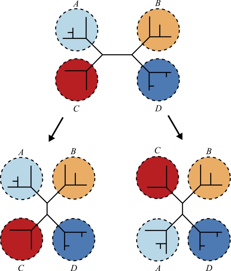
For a tree toplogy that contains four or more taxa, the Nearest Neighbor Interchange (NNI) exchanges subtrees within the larger tree. It can be shown that for a tree with four subtrees there are only 3 distinct ways to exchange subtrees to create a new tree, including the original tree. Therefore, each such application produces two new trees that are different from the input tree [50 51].

Subtree Pruning and Regrafting

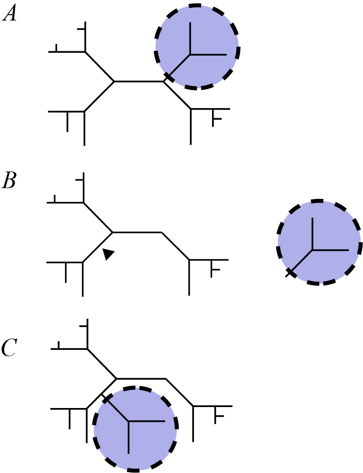
The Subtree Pruning and Regrafting (SPR) method takes a subtree from a larger tree, removes it and reattaches it to another part of the tree [52 53].

4.4 Lab 5: Phylogenetics

In this lab, we will learn some basic commands for computing phylogenetic trees, and some python commands that will draw the tree. Let’s create a new directory called [latex]\texttt{Lab5}[/latex] to work in.

4.4.1 Download Sequences from NCBI

Download sequences in FASTA format for a gene of interest from NCBI nucleotide (https://www.ncbi.nlm.nih.gov/nuccore). Build a FASTA file containing each sequence and a defline. Shorten the defline for each species to make it easier to read later. As an example, I downloaded 18S rRNA for Human (Homo sapiens), Mouse (Mus musculus), Rat (Rattus norvegicus), Frog (Xenopus laevis), Chicken (Gallus gallus), Fly (Drosophila melanogaster) and Arabidopsis (Arabidopsis thalian). You can download these 18S rRNA sequences with the following command:

$ wget http://hendrixlab.cgrb.oregonstate.edu/teaching/18S_rRNAs.fasta


4.4.2 Create a Multiple Sequence Alignment and Phylogenetic Tree with Clustal

First, use [latex]\texttt{clustalw2}[/latex] to align the sequences, and output a multiple sequence alignment and dendrogram file.

$ clustalw2 -infile=18S_rRNAs.fasta -type=DNA -outfile=18S_rRNAs.aln

The dendogram file, indicated by the “[latex]\texttt{.dnd}[/latex]” suffix, can be used to create an image of a phylogenetic tree using Biopython: First, enter the python terminal by typing “[latex]\texttt{.python}[/latex]” and then the following:

>>> import matplotlib as mpl
>>> mpl.use('Agg')
>>> import matplotlib.pyplot as pyplot
>>> from Bio import Phylo
>>> tree = Phylo.read('18S_rRNAs.dnd','newick')
>>> Phylo.draw(tree)
>>> pyplot.savefig("myTree.png")
>>> quit()
 

How does the resulting tree compare to what you expect given these species?

4.4.3 Create a Multiple Sequence Alignment and Phylogenetic Tree with phyML

The program phyML provides much more flexibility in what sort of trees it can compute. To use it, we’ll need to convert our alignment file to phylip. We can do this with the Biopython module AlignIO

>>> from Bio import AlignIO
>>> alignment = AlignIO.parse("18S_rRNAs.aln","clustal")
>>> AlignIO.write(alignment,open("18S_rRNAs.phy","w"),"phylip")
1
>>> quit()

You can run phyml in the simplest way by simply typing “phyml” and then typing your alignment file:

$ phyml

    Enter the sequence file name > 18S_rRNAs.phy

The program will give you a set of options, and you can optionally change them. To change the model, type “+” and then “M” to toggle through the models. Finally, hit “enter” to run the program.

>>> import matplotlib as mpl
>>> mpl.use('Agg')
>>> import matplotlib.pyplot as pyplot
>>> from Bio import Phylo
>>> tree = Phylo.read('18S_rRNAs.phy_phyml_tree.txt','newick')
>>> Phylo.draw(tree)
>>> pyplot.savefig("myTreeML.png")
>>> quit()

How does the tree created from [latex]\texttt{clustalw2}[/latex] compare to the tree created using [latex]\texttt{phyml}[/latex]?