2 Utility

The Policy Question
Is a tax credit on hybrid car purchases the government’s best choice to reduce fuel consumption and carbon emissions?

US residents and the government are concerned about the dependence on imported foreign oil and the release of carbon into the atmosphere. In 2005, Congress passed a law to provide consumers with tax credits toward the purchase of electric and hybrid cars.

This tax credit may seem like a good policy choice, but it is costly because it directly lowers the amount of revenue the US government collects. Are there more effective approaches to reducing dependency on fossil fuels and carbon emissions? How do we decide which policy is best? To answer this question, policymakers need to predict with some accuracy how consumers will respond to this tax policy before these policymakers spend millions of federal dollars.

We can apply the concept of utility to this policy question. In this chapter, we will study utility and utility functions. We will then be able to use an appropriate utility function to derive indifference curves that describe our policy question.

Exploring the Policy Question

1. Suppose that the tax credit to subsidize hybrid car purchases is wildly successful and doubles the average fuel economy of all cars on US roads—a result that is clearly not realistic but useful for our subsequent discussions. What do you think would happen to the fuel consumption of all US motorists? Should the government expect fuel consumption and carbon emissions from cars to decrease by half in response? Why or why not?

2.1 Utility Functions

Learning Objective 2.1: Describe a utility function.

Our preferences allow us to make comparisons between different consumption bundles and choose the preferred bundles. We could, for example, determine the rank ordering of a whole set of bundles based on our preferences. A utility function is a mathematical function that ranks bundles of consumption goods by assigning a number to each, where larger numbers indicate preferred bundles. Utility functions have the properties we identified in chapter 1 regarding preferences. That is, they are able to order bundles, they are complete and transitive, more is preferred to less, and in relevant cases, mixed bundles are better.

The number that the utility function assigns to a specific bundle is known as utility, the satisfaction a consumer gets from a specific bundle. The utility number for each bundle does not mean anything in absolute terms; there is no uniform scale against which we measure satisfaction. Its only purpose is in relative terms: we can use utility to determine which bundles are preferred to others.

If the utility from bundle [latex]A[/latex] is higher than the utility from bundle [latex]B[/latex], it is equivalent to saying that a consumer prefers bundle [latex]A[/latex] to bundle [latex]B[/latex]. Utility functions, therefore, rank consumer preferences by assigning a number to each bundle. We can use a utility function to draw the indifference curve maps described in chapter 1. Since all bundles on the same indifference curve provide the same satisfaction and therefore none is preferred, each bundle has the same utility. We can therefore draw an indifference curve by determining all the bundles that return the same number from the utility function.

Economists say that utility functions are ordinal rather than cardinal. Ordinal means that utility functions only rank bundles—they only indicate which one is better, not how much better it is than another bundle. Suppose, for example, that one utility function indicates that bundle[latex]A[/latex] returns ten utils and bundle[latex]B[/latex]twenty utils. We do not say that bundle [latex]B[/latex] is twice as good, or ten utils better, only that the consumer prefers bundle [latex]B[/latex]. For example, suppose a friend entered a race and told you she came in third. This information is ordinal: You know she was faster than the fourth-place finisher and slower than the second-place finisher. You only know the order in which runners finished. The individual times are cardinal: if the first-place finisher ran the race in exactly one hour and your friend finished in one hour and six minutes, you know your friend was exactly 10 percent slower than the fastest runner. Because utility functions are ordinal, many different utility functions can represent the same preferences. This is true as long as the ordering is preserved.

Take, for example, the utility function [latex]U[/latex] that describes preferences over bundles of goods [latex]A[/latex] and [latex]B[/latex]: [latex]U(A,B)[/latex]. We can apply any positive monotonic transformation to this function (which means, essentially, that we do not change the ordering), and the new function we have created will represent the same preferences. For example, we could multiply a positive constant, [latex]\alpha[/latex], or add a positive or a negative constant, [latex]\beta[/latex]. So [latex]\alpha U(A,B)+ \beta[/latex] represents exactly the same preferences as [latex]U(A,B)[/latex] because it will order the bundles in exactly the same way. This fact is quite useful because sometimes applying a positive monotonic transformation of a utility function makes it easier to solve problems.

2.2 Utility Functions and Typical Preferences

Learning Objective 2.2: Identify utility functions based on the typical preferences they represent.

Consider bundles of apples, [latex]A[/latex], and bananas, [latex]B[/latex]. A utility function that describes Isaac’s preferences for bundles of apples and bananas is the function [latex]U(A,B)[/latex]. But what are Isaac’s particular preferences for bundles of apples and bananas? Suppose that Isaac has fairly standard preferences for apples and bananas that lead to our typical indifference curves: he prefers more to less, and he likes variety. A utility function that represents these preferences might be

[latex]U(A,B) = AB[/latex]

If apples and bananas are perfect complements in Isaac’s preferences, the utility function would look something like this:

[latex]U(A,B) = MIN[A,B][/latex]

where the [latex]MIN[/latex] function simply assigns the smaller of the two numbers as the function’s value.

If apples and bananas are perfect substitutes, the utility function is an additive and would look something like this:

[latex]U(A,B) = A + B[/latex]

Cobb-Douglas utility functions are commonly used in economics for two reasons:

1. They represent standard preferences, such as more is better and preference for variety.
2. They are very flexible and can be adjusted to fit real-world data very easily.

Cobb-Douglas utility functions have this form:

[latex]U(A,B) = A^\alpha B^\beta[/latex]

Because positive monotonic transformations represent the same preferences, one such transformation can be used to set [latex]\alpha + \beta = 1[/latex], which later we will see is a convenient condition that simplifies some math in the consumer choice problem.

Another way to transform the utility function in a useful way is to take the natural log of the function, which creates a new function that looks like this:

[latex]U(A,B) = \alpha ln(A) + \beta ln(B)[/latex]

To derive this equation, simply apply the rules of natural logs. It is important to keep in mind the level of abstraction here. We typically cannot make specific utility functions that precisely describe individual preferences. Probably none of us could describe our own preferences with a single equation. But as long as consumers in general have preferences that follow our basic assumptions, we can do a pretty good job finding utility functions that match real-world consumption data. We will see evidence of this later in the course.

2.3 Relating Utility Functions and Indifference Curve Maps

Learning Objective 2.3: Explain how to derive an indifference curve from a utility function.

Indifference curves and utility functions are directly related. In fact, since indifference curves represent preferences graphically and utility functions represent preferences mathematically, it follows that indifference curves can be derived from utility functions.

In univariate functions, the dependent variable is plotted on the vertical axis, and the independent variable is plotted on the horizontal axis, like the graph of [latex]y=f(x)[/latex]. In contrast, graphs of bivariate functions are three-dimensional, like [latex]U=U(A,B)[/latex]. Figure 2.1 shows a graph of [latex]U=A^\frac{1}{2}B^\frac{1}{2}[/latex]. Three-dimensional graphs are useful for understanding how utility increases with the increased consumption of both A and B.

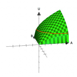
Figure 2.1 clearly shows the assumption that consumers have a preference for variety. Each bundle, which contains a specific amount of [latex]A[/latex] and [latex]B[/latex], represents a point on the surface. The vertical height of the surface represents the level of utility. By increasing both [latex]A[/latex] and [latex]B[/latex], a consumer can reach higher points on the surface.

So where do indifference curves come from? Recall that an indifference curve is a collection of all bundles that a consumer is indifferent about with respect to which one to consume. Mathematically, this is equivalent to saying all bundles, when put into the utility function, return the same functional value. So if we set a value for utility, [latex]Ū[/latex], and find all the bundles of [latex]A[/latex] and [latex]B[/latex] that generate that value, we will define an indifference curve. Notice that this is equivalent to finding all the bundles that get the consumer to the same height on the three-dimensional surface in figure 2.1.

Indifference curves are a representation of elevation (utility level) on a flat surface. In this way, they are analogous to a contour line on a topographical map. By taking the three-dimensional graph back to two-dimensional space—the A, B space—we can show the contour lines / indifference curves that represent different elevations or utility levels. From the graph in figure 2.1, you can already see how this utility function yields indifference curves that are “bowed-in” or concave to the origin.

So indifference curves follow directly from utility functions and are a useful way to represent utility functions in a two-dimensional graph.

2.4 Finding Marginal Utility and Marginal Rate of Substitution

Learning Objective 2.4: Derive marginal utility and MRS for typical utility functions.

Marginal utility [latex](MU)[/latex] is the additional utility a consumer receives from consuming one additional unit of a good. Mathematically, we express this as

[latex]MU_{A}=\frac{\Delta U}{\Delta A}[/latex]

or the change in utility from a change in the amount of [latex]A[/latex] consumed, where Δ represents a change in the value of the item, so

[latex]MU_{A}=\frac{\Delta U}{\Delta A}=\frac{U (A+\Delta A,B)-U(A,B)}{\Delta A}[/latex]

Note that when we are examining the marginal utility of the consumption of [latex]A[/latex], we hold [latex]B[/latex] constant.

Using calculus, the marginal utility is the same as the partial derivative of the utility function with respect to [latex]A[/latex]:

[latex]MU_{A}=\frac{\partial U(A,B)}{\partial A}[/latex]

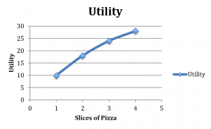
Consider a consumer who sits down to eat a meal of salad and pizza. Suppose that we hold the amount of salad constant—one side salad with a dinner, for example. Now let’s increase the slices of pizza; suppose with one slice, utility is ten; with two, it is eighteen; with three, it is twenty-four; and with four, it is twenty-eight. Let’s plot these numbers on a graph that has utility on the vertical axis and pizza on the horizontal axis (table 2.2 and figure 2.2).

Table 2.2 Diminishing marginal utility

Pizza slices	Utility	Marginal utility
1	10
2	18	8
3	24	6
4	28	4

From the positive slope of the graph, we can see the increase in utility from additional slices of pizza. From the concave shape of the graph, we can see another common phenomenon: the additional utility the consumer receives from each additional slice of pizza decreases with the number of slices consumed.

The fact that the additional utility gets smaller with each additional slice of pizza is called the principle of diminishing marginal utility. This principle applies to well-behaved preferences where mixed bundles are preferred.

Marginal rate of substitution (MRS) is the amount of one good a consumer is willing to give up to get one more unit of another good. This is why it is the same thing as the slope of the indifference curve—since we keep satisfaction level constant, we stay on the same indifference curve, just moving along it as we trade one good for another. How much of one you are willing to trade for one more of another depends on the marginal utility of each.

Using our previous example, if by consuming one more side salad, your utility goes up by ten, then at a current consumption of four slices of pizza, you could give up two slices of pizza and go from twenty-eight to eighteen utils. Ten more utils from salad and ten fewer utils by giving up two slices of pizza leave overall utility unchanged—so we must still be on the same indifference curve. As you move along the indifference curve, you must be riding the slope—that is, you must be giving up the good on the vertical axis for more of the good on the horizontal axis, which yields a negative rise over a positive run.

We can go directly from marginal utility to[latex]MRS[/latex] by recognizing the connection between the two concepts. In our case, for the utility function [latex]U=U(A,B)[/latex], [latex]MRS[/latex] is represented as

[latex]MRS=-\frac{MU_{A}}{MU_{B}}[/latex]

Note that when we substitute, we can simplify the equation:

[latex]MRS=-\frac{MU_{A}}{MU_{B}}=-\frac{\frac{\Delta U}{\Delta A}}{\frac{\Delta U}{\Delta B}}=-\frac{\Delta B}{\Delta A}[/latex]

Inserting the calculus it equates to

[latex]MRS=-\frac{\frac{\partial U(A,B)}{\partial A}}{\frac{\partial U(A,B)}{\partial B}}[/latex]

2.5 The Policy Example
Is a tax credit on hybrid car purchases the government’s best choice to reduce fuel consumption and carbon emissions?

We determined in chapter 1 that the relevant consumer decision between more miles driven and other consumption probably conforms to the standard assumptions about consumer choice. Therefore, using the Cobb-Douglas utility function to represent a consumer who likes to drive a car as well as consume other goods and who sees them as a trade-off (money spent on gas is money not spent on other consumer goods) is a good choice. It also has the benefits of both conforming to the assumptions and being flexible:

[latex]U(MD,C)=MD^{a}C^{\beta }[/latex]

where [latex]MD[/latex] = miles driven and [latex]C[/latex]= other consumption.

In fact, the function itself can be taken to real-world data, where the parameters can be estimated for this market, the market for miles driven in the consumer’s car.

Exploring the Policy Question

1. Would other preference types be more appropriate in this example?
2. What would have to be true for perfect complements to be the appropriate preference type to use to analyze this policy?
3. What would have to be true for perfect substitutes? Given that we are considering a “typical” consumer who drives, is it appropriate to choose a “typical” utility function?
4. Are we just guessing, or do we have some basis in theory to support our choice of “well-behaved” preferences or a Cobb-Douglas utility function?

REVIEW: TOPICS AND RELATED LEARNING OUTCOMES

2.1 Utility Functions

Learning Objective 2.1: Describe a utility function.

2.2 Utility Functions and Typical Preferences

Learning Objective 2.2: Identify utility functions based on the typical preferences they represent.

2.3 Relating Utility Functions and Indifference Curve Maps

Learning Objective 2.3: Explain how to derive an indifference curve from a utility function.

2.4 Finding Marginal Utility and Marginal Rate of Substitution

Learning Objective 2.4: Derive marginal utility and MRS for typical utility functions.

2.5 Policy Example
Is a Tax Credit on Hybrid Car Purchases the Government’s Best Choice?

Learning Objective 2.5: The Hybrid Tax Credit and customer utility

LEARN: KEY TOPICS

Terms

Utility

The number that a utility function assigns to a specific bundle.

Univariate functions

The dependent variable is plotted on the vertical axis and the independent variable is plotted on the horizontal axis, i.e., the graph of [latex]f(x)=mx+b[/latex].

Bivariate functions

Functions containing two potentially independent variables. If one variable is influencing another variable, then you will have bivariate data that has an independent and dependent variable.

Useful for understanding how utility increases with the increased consumption of both [latex]A[/latex] and [latex]B[/latex], i.e., the graph of [latex]U=A^\frac{1}{2}B^\frac{1}{2}[/latex].

Ordinal

A function that deals in ranking as opposed to pure quantification; they only indicate which bundle is better, more preferred, etc., but not how much better it is than another bundle. After application of positive monotonic transformation to an ordinal function, meaning the ordering is not changed, the new function will represent the same preferences. If an ordinal function is reported in utils, regardless of the amounts used there is no relationship implied, i.e., bundle [latex]A[/latex] having 10 utils and bundle [latex]B[/latex] having 20 utils does not imply bundle [latex]B[/latex] is two times as preferred as bundle [latex]A[/latex], only that it is more preferred.

Cardinal

The utility of the product measured with the help of the product’s weight, length, temperature, etc.

Util

A unit used to transform the logical utility of a product to empirical. The ordinal utility might say that the consumer prefers the apple to the orange. Cardinal utility might say that the apple provides 80 utils while the orange only provides 40 utils.

Contour line

A way to represent a 3-dimensional topographical map in a two-dimensional space.

Diminishing marginal utility

The additional utility a customer receives from a product diminishes with each additional iteration of the product the customer receives.

Example

Table 2.2 Diminishing marginal utility

Total pizza slices consumed	Utility	Marginal utility
1 slice	10	N/A; no margin
2 slices	18	8
3 slices	24	6
4 slices	28	4

Table 2.2 Diminishing marginal utility

Pizza slices	Utility	Marginal utility
1	10
2	18	8
3	24	6
4	28	4

As a customer consumes more and more slices of pizza, the additional utility having one more slice of pizza provides–satiating excess hunger, producing dopamine from a delicious flavor, etc.–decreases with each additional slice.

Graph

3D utility function and contour line

Equations

Cobb-Douglas utility function

A utility function describing goods which are neither complements nor substitutes.

[latex]U(A,B) = A^\alpha B^\beta[/latex]

Perfect complement utility function

A utility function that describes goods that are perfect complements. See table 2.1 for more details.

[latex]U(A,B) = MIN[A,B][/latex]

Perfect substitute utility function

A utility function that describes goods that are perfect substitutes. See table 2.1 for more details.

[latex]U(A,B) = A + B[/latex]

Marginal rate of substitution [latex](MRS)[/latex]

[latex]MRS=-\frac{MU_{A}}{MU_{B}}[/latex]

Defined as the amount of one good a consumer is willing to give up to get one more unit of another good.

From [latex]MU[/latex] to [latex]MRS[/latex]

There is a direct connection between marginal utility and the marginal rate of substitution. This connection varies somewhat by utility function. From our basic utility function, [latex]U=U(A,B)[/latex], [latex]MRS[/latex] is represented as

[latex]MRS=-\frac{MU_{A}}{MU_{B}}[/latex]

Substitution results in the following simplification:

[latex]MRS=-\frac{MU_{A}}{MU_{B}}=-\frac{\frac{\Delta U}{\Delta A}}{\frac{\Delta U}{\Delta B}}=-\frac{\Delta B}{\Delta A}[/latex]

Utilizing calculus:

[latex]MRS=-\frac{\frac{\partial U(A,B)}{\partial A}}{\frac{\partial U(A,B)}{\partial B}}[/latex]

Marginal utility [latex](MU)[/latex]

[latex]MU_{a}=\frac{\Delta U}{\Delta A}[/latex]

The additional utility a consumer receives from consuming one additional unit of a good.

Utility function

Functions that rank bundles of consumption goods by assigning a number to each, where larger numbers indicate preferred bundles.

Table Summarizing Utility Functions

Table 2.1 Types of preferences and the utility functions that represent them

Preferences	Utility function	Type of utility function
Love of variety or “well behaved”	[latex]U(A,B)=AB[/latex]	Cobb-Douglas
Love of variety or “well behaved”	[latex]U(A,B)=A^\alpha B^\beta[/latex]	Cobb-Douglas
Love of variety or “well behaved”	[latex]U(A,B)=\alpha ln(A)+\beta ln(B)[/latex]	Natural log Cobb-Douglas
Perfect complements	[latex]U(A,B) = MIN[A,B][/latex]	Min function
Perfect substitutes	[latex]U(A,B)=A+B[/latex]	Additive