Chapter 7: Noncoding RNAs
It was once believed that most genes encode proteins and most transcripts are messenger RNAs (mRNAs). According to some studies on the matter, the number of genes that do not encode proteins outnumbers those that do [63]. Unlike mRNAs, which are translated into proteins by the ribosome, these noncoding RNAs (ncRNAs) act functionally as an RNA transcript. NcRNAs that are greater than 200nt are called long noncoding RNAs (lncRNAs), and those that are less than 50nt can be called small noncoding RNAs (sncRNAs). The remaining intermediate size range from 50-199nt can be called short RNAs, although these exact length thresholds are a bit arbitrary.
7.1 Small Noncoding RNAs (srcRNAs)
As we learned in Chapter 6, the transcriptome includes small transcripts. These sncRNAs are involved in gene regulation and gene silencing, regulation of splicing, and possibly other epigenetic roles throughout the cell. Many sncRNAs act as guides to direct the sequence-specific activity of enzymes to other RNAs such as mRNAs or other transcripts. Other more recent studies have implicated sncRNAs in directing the binding to DNA through triplex interactions.
7.1.1 microRNAs
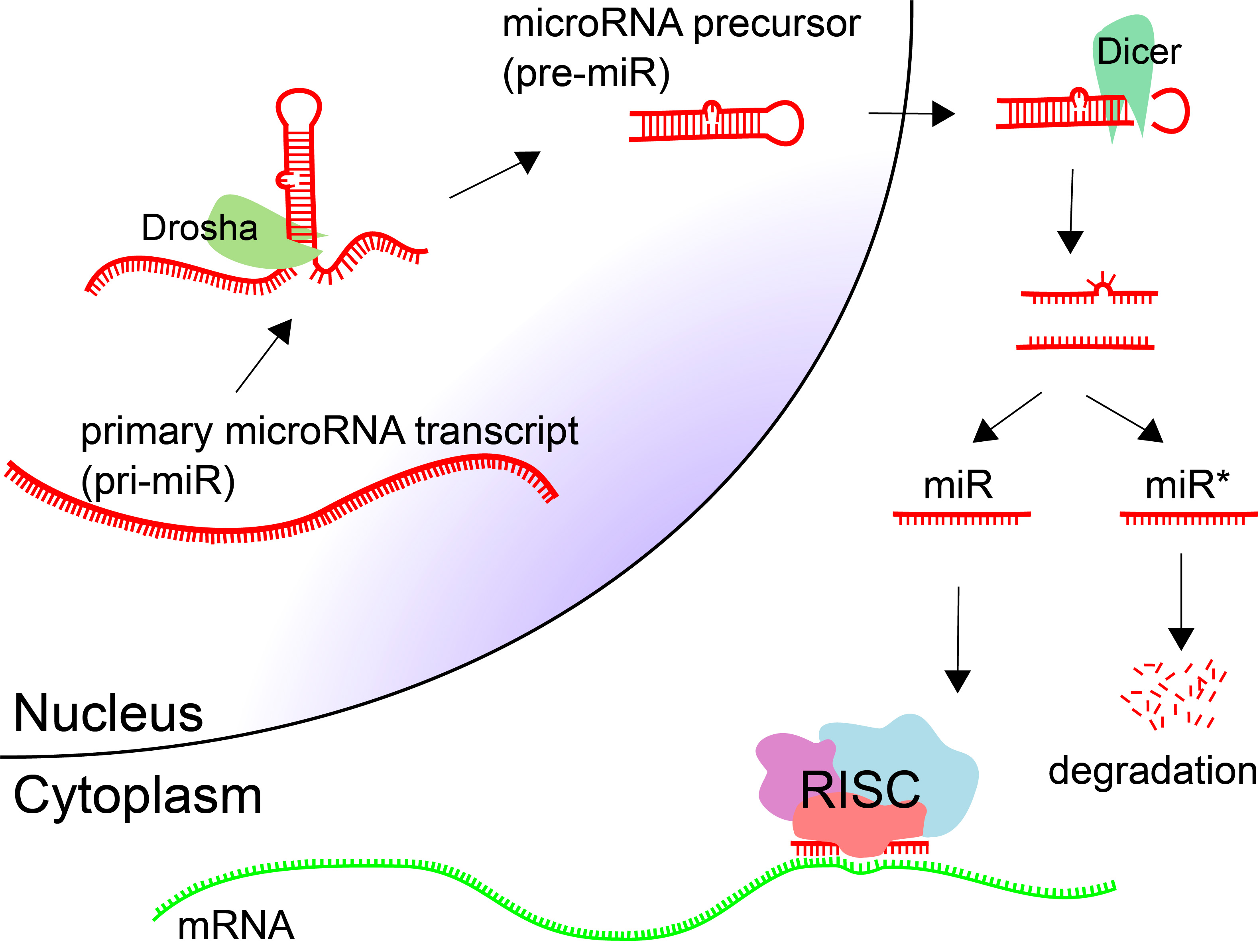
MicroRNAs (miRNAs, miRs) are small endogenous regulatory RNA molecules (18-25nt) that are involved in post-transcriptional gene silencing [64]. miRNAs are processed from longer primary transcripts. Hairpins are cut at the base by Drosha, producing a microRNA precursor (pre-miR). These hairpin precursors are shuttled out of the nucleus and cut at the loop to produce double-stranded RNA. Typically one of the products is incorporated into the RNA-induced silencing complex (RISC), and the other is degraded.
Target sites for microRNAs are in the 3' UTR of protein coding genes, although they have been observed in protein-coding regions as well. The target sites are around 7 nt in length, complementary to positions 2-8 of the mature microRNA.
7.1.2 piRNAs
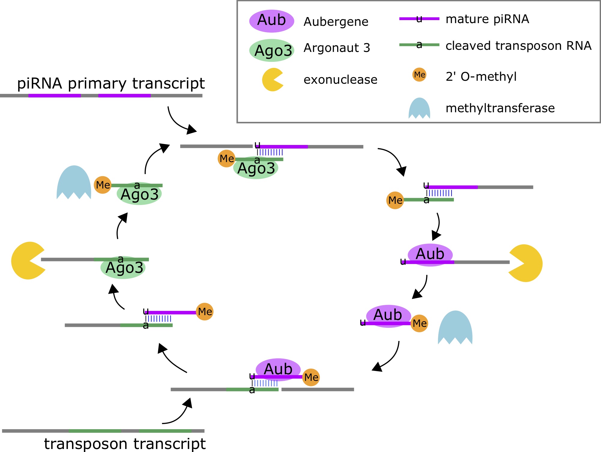
Piwi-interacting RNAs (piRNAs, piRs) are small endogenous RNAs molecules (21-31nt) that are part of the genome's natural defense against transposons, and may be involved in post-transcriptional gene silencing and other epigenetic functions [65]. piRNAs are the most abundant class of small RNAs [66]. piRNAs are processed from longer primary transcripts based on complementary interactions with transposon transcripts. These small RNAs do not arise from hairpins, but rather the duplex interactions with the transposon transcripts. The enzymes Aubergene (Aub) and Argonaute 3 (Ago3) for processing [67]. Ago3 cuts the piRNA primary transcript by using a transposon-derived small RNA as a guide, and Aub cuts the transposon transcript using a mature piRNA as a guide.
7.1.3 Duplex RNA interactions
Many small RNAs function through the RNA duplex formation due to complementary sequence interactions. Let's discuss how we can describe these types of interactions.
Consider the complementary RNA sequences [latex]A=\texttt{ACGCAUU}[/latex] and [latex]B=\texttt{AAUGCGU}[/latex] that could form a base-paired (heterodimeric) RNA duplex [latex]A:B[/latex].
5' ACGCAUU 3'

|||||||

3' UGCGUAA 5'
The reaction for this duplex formation could be expressed as follows:
[latex]A + B \rightleftharpoons A:B[/latex]
This is under the assumption that there are no structures formed by [latex]A[/latex] and [latex]B[/latex] on their own that need to unfold for the reaction to proceed forward, and that the individual molecules [latex]A[/latex] and [latex]B[/latex] don't form homodimers on their own. In many applications, this equation is depicted the other way, and the process is described as a "melting" process whereby the duplex becomes unpaired.
[latex]A:B \rightleftharpoons A+B[/latex]
| Sequence | [latex]\Delta G[/latex] (kcal/mol) |
|---|---|
| AA:UU | -0.93 |
| AU:AU | -1.10 |
| UA:UA | -1.33 |
| CA:UG | -2.11 |
| GU:AC | -2.24 |
| CU:AG | -2.08 |
| GA:UC | -2.35 |
| CG:CG | -2.36 |
| GC:GC | -3.42 |
| GG:CC | -3.26 |
| GC-init. | 2.045 |
| AU-init | 2.495 |
| symm | 0.43 |
The energy required to drive such a reaction is set by the equilibrium constant for this reaction
[latex]K = \frac{[A][B]}{[AB]}[/latex]
And the free energy required to melt the duplex is given by
[latex]\Delta G = -RT \ln ( K ) = -RT \ln \frac{[A][B]}{[AB]}[/latex]
The temperature at which the paired and unpaired nucleotides become equally abundant is defined as the melting temperature
[latex]T_m = - \frac{\Delta G}{R \ln ([AB]_0 /2)}[/latex]
In our example above, the RNA duplex with sequences [latex]A=\texttt{ACGCAUU}[/latex] and [latex]B=\texttt{AAUGCGU}[/latex] forms a duplex. Since this system is completely paired, we can describe it as a sequence of base pairs [latex]b_i[/latex], corresponding to the base pair at position $i$. In this example, using 1-based coordinates, we have [latex]b_1 = A : U[/latex]. The nearest neighbor model describes the basepair energy between a duplex as the sum of dimer interactions, plus initialization terms on the ends. The full expression for the duplex energy is then
[latex]\Delta G = \Delta G_{init}(b_1) + \Delta G_{init} (b_n) + \sum_{i=1}^{n-1} \Delta G(b_i,b_{i+1})[/latex]
Calculating Duplex Energy with the Nearest Neighbor Model
Let's consider an example. [latex]A=\texttt{UCAGG}[/latex] and [latex]B=\texttt{CCUGA}[/latex]. In this case, the
[latex]\Delta G(A:B) = \Delta G_{init}(\texttt{U:A}) + \Delta G_{init} (\texttt{C:G}) + \sum_{i=1}^{n-1} \Delta G(b_i,b_{i+1})[/latex]
[latex]\Delta G(A:B) = 2.495 + 2.045 + \sum_{i=1}^{n-1} \Delta G(b_i,b_{i+1})[/latex]
The summation terms can be expanded as follows
[latex]\sum_{i=1}^{n-1} \Delta G(b_i,b_{i+1}) = \Delta G(\texttt{UC:GA}) + \Delta G(\texttt{CA:UG}) + \Delta G(\texttt{AG:CU}) + \Delta G(\texttt{GG:CC})[/latex]
[latex]\sum_{i=1}^{n-1} \Delta G(b_i,b_{i+1}) = -2.35 - 2.11 - 2.08 - 3.26[/latex]
Adding up all the terms gives the final solution.
[latex]\Delta G(A:B) = -5.26 kcal/mol[/latex]
7.1.4 RNA/DNA Hybrids
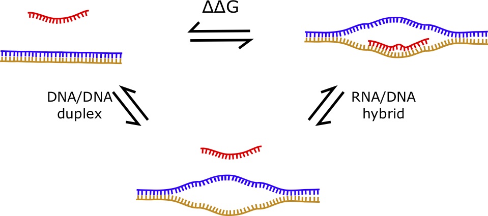
RNA/DNA hybrids are structures formed by a "hybrid duplex" consisting of one strand of RNA and one strand of DNA [68, 69]. If was assume that the RNA has no structure (i.e. is a sncRNA) and that the DNA doesn't fold into a structure when the double helix is opened, the energy parameters of such an interaction can be computed using the difference between the DNA/DNA duplex energy and the RNA/DNA hybrid energy. The [latex]\Delta \Delta G[/latex] can be computed from the difference of these two values. Therefore, the formula is given by:
[latex]\Delta \Delta G = \Delta G_{hybrid} - \Delta G_{DNA duplex}[/latex]
| first →
second ↓ |
G | C | A | T |
|---|---|---|---|---|
| G | -1.84 | -2.17 | -1.28 | -1.45 |
| C | -.2.24 | -1.84 | -1.44 | -1.30 |
| A | -1.3 | -1.45 | -1.00 | -0.58 |
| T/U | -1.44 | -1.28 | -0.88 | -1.00 |
| G | C | A | U |
|---|---|---|---|
| -2.2 | -1.2 | -1.4 | -1.0 |
| -2.4 | -1.5 | -1.6 | -0.8 |
| -1.4 | -1.0 | -0.4 | -0.3 |
| -1.5 | -0.9 | -1.0 | -0.2 |
| first →
second ↓ |
G | C | A | T |
|---|---|---|---|---|
| G | -0.36 | 0.97 | -0.12 | 0.445 |
| C | -0.16 | 0.34 | -0.16 | 0.5 |
| A | -0.1 | 0.45 | 0.6 | 0.28 |
| T/U | -0.06 | 0.38 | -0.12 | 0.8 |
7.1.5 Triplexes
Triple-helix (triplex) structures between a double-stranded nucleic acid sequence and a single-stranded nucleic acid sequence can form for specific triplets of nucleotides. For example, triplexes can form between a single-stranded RNA sequence and double-stranded DNA. The energy parameters of these interactions are not known, but interactions can be predicted with a program like [latex]\texttt{Triplexator}[/latex]: http://bioinformatics.org.au/tools/triplexator/
$ triplexator -l 15 -e 20 -o output.txt -ss transcripts.fasta -ds promoters.fasta
The output, stored to the file specified by the [latex]\texttt{-o}[/latex] flag, is a tab-delimited file containing information on the locations of triplex forming oligonucleotides (TFOs) [70].
7.2. Long Noncoding RNAs
7.2.1 Quantifying coding potential
In order to identify noncoding RNAs, perhaps it is easier to characterize what is coding, and label the remaining as noncoding. Many approaches have been developed to quantify a transcripts potential to encode a protein ranging from comparative approaches, to machine learning, to experimental methods.
Coding Potential and Homology
The first approach is to use homology, such as by BLAST or using protein domains on predicted ORFs. If there is significant homology between the translation of an ORF and a known protein, then there is a good chance that the gene in question is also protein coding. Similarly, if an ORF translates to a sequence that has a known protein domain, then it is likely protein coding.
However, the caveat here is to make sure that the gene has a valid, functional ORF. If a mutation has caused the ORF to be lost (e.g. introduce an early stop codon or several frame-shifts) then there is a good chance it is a "pseudogene", which could be considered noncoding.
Evolutionary Models
Evolutionary methods for identifying coding potential rely on the fact that protein coding genes have well defined sequences of codons, which constitute an open reading frame. Open reading frames (ORFs) are defined by a start codon positioned at a multiple of three nucleotides away from a stop codon. When considered comparatively across different species in a multiple alignment, one rarely sees nucleotide insertions or deletions that cause a "frame shift". Frame shifts are when the phase of the codons changes, giving rise to a transcript that encodes a completely different amino acid sequence, if at all. Similarly, multiple sequence alignments of protein coding transcripts are depleted for mutations that cause a non-synonymous change, or mutations that alter what amino acid a codon encodes. The software PhyloCSF does exactly this, and quantifies the likelihood of a given transcripts being coding or noncoding based on its multiple alignment [71].
Machine Learning Approaches to Coding Potential
Machine learning approaches define a set of "features" that describe the phenomena that the program seeks to learn. For identifying protein coding genes, the features describe aspects of the transcript being evaluated. For example, the program [latex]\texttt{CPAT}[/latex] (Coding Potential Assessment Tool) quantifies the frequencies of [latex]K[/latex]-mers in the transcript, as well as the length of the transcript, and is able to distinguish protein coding genes from noncoding fairly well [72].
Ribosome Binding Profiles
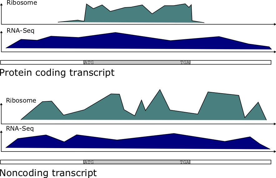
Ribosomal profiling quantifies the binding of the Ribosome to transcripts at each position. It has been determined that protein coding genes have a distinct ribosomal profile over the open reading frame, characterized by a sharp drop-off in binding immediately after the stop codon. Noncoding RNAs have a more stochastic binding profile around trinucleotides matching the stop codon at the end of an (untranslated) ORF [73]. Figure 7.4 depicts the kind of data produced in these experiments. To quantify the potential for coding, the authors developed a score called a Ribosomal Release Score (RRS). The equation for the RRS is
[latex]RRS = \frac{ \left( C_{CDS} / C_{3'UTR} \right)_{Ribosome} }{ \left( C_{CDS}/C_{3'UTR} \right)_{RNA-seq}}[/latex]
(7.1)
For protein coding genes, we expect this ribosome ratio to be high, since the Ribosome read count [latex]C_{CDS}[/latex] should be much greater than that of [latex]C_{3'UTR}[/latex] for such genes.
Detecting Peptides with Mass Spectrometry
Some approaches have used Mass Spectrometry to detect small peptides, and validate that a particular open reading frame was real. In these cases, small peptides can be detected that were predicted to be translated from a small ORF [74].
7.3 RNA Structure Prediction
Many ncRNAs operate by forming a structure, consisting of basepairs between nucleotides (formed by hydrogen bonds), as well as regions of unpaired nucleotides. An RNA structure can be viewed at many different levels, with the "primary structure" consisting of the sequence itself. The secondary structure consists of a mapping of which nucleotides are paired, and can be represented on a 2D surface. The tertiary structure consists of the three dimensional configuration of the molecule. The quaternary structure comprises the inter-molecular interactions that these molecules can participate in.
While the primary structure of the RNA can be described by a sequence [latex]r[/latex] of the characters [latex]\{A,C,G,U\}[/latex], such that [latex]r[i][/latex] corresponds the the nucleotide at position [latex]i[/latex] of the molecule the sequence represents. The secondary structure can be represented by a set of ordered pairs [latex]S[/latex] such that each pair of positions [latex]i j[/latex] that form a base pair constitutes an ordered pair [latex](i,j) \in S[/latex], and the corresponding nucleotides [latex]r[i][/latex] and [latex]r[j][/latex] are complementary. One could remove restriction that i<j, then you could consider the basepairs unordered pairs [latex]\{i,j\}[/latex].
7.3.1 The Nussinov Algorithm
The Nussinov Algorithm predicts the number of basepairs, and ultimately the structure for an RNA sequence using dynamic programming [75]. This is done by understanding that whether or not a pair of nucleotides [latex]i,j[/latex] will pair depends on the intervening nucleotides from [latex]i+1[/latex] to [latex]j-1[/latex].
Let's consider an RNA sequence [latex]r[/latex] with nucleotides [latex]r[i][/latex]. Consider the possible base pair formed between positions [latex]i[/latex] and [latex]j[/latex]. This will of course depend on whether [latex]r[i][/latex] and [latex]r[j][/latex] are complementary or wobble pairs capable of forming hydrogen bonds.
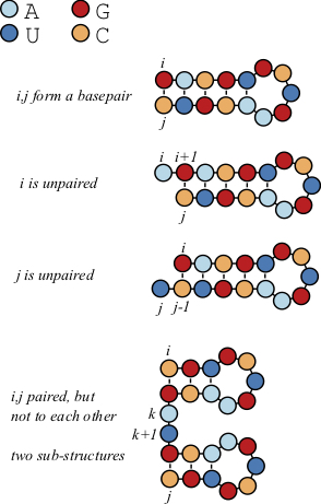
Let's build a scoring matrix [latex]B[/latex] such that the terms of this matrix [latex]B_{ij}[/latex] correspond to the number of basepairs between these two positions.
[latex]\begin{aligned} B_{i,j} = max \begin{cases} B_{i+1,j-1} + 1& \mbox{$i$ and $j$ are paired}\\ B_{i+1,j} & \mbox{$i$ unpaired, use structure from $i+1$ to $j$}\\ B_{i,j-1} & \mbox{$j$ unpaired, use structure from $i$ to $j-1$}\\ max_{i k j} \{ B_{i,k} + B_{k+1,j} \} & \mbox{bifurcation} \\ \end{cases} \end{aligned}[/latex]
(7.2)
The first three options are probably pretty clear. Either it adds a basepair at [latex]i,j[/latex], or it doesn't. If it adds a basepair, then increment [latex]+1[/latex] to the previous value [latex]B_{i+1,j-1}[/latex], that corresponds to the best structure prediction for the intervening positions.
If it doesn't add a pair, then simply extend a previously computed number of basepairs to [latex]B_{ij}[/latex].
The fourth term is the most complex. In this condition, there is an intermediate nucleotide [latex]k[/latex], such that the structures produced from [latex]i[/latex] to [latex]k[/latex] and from [latex]k+1[/latex] to [latex]j[/latex] are optimal. After going through all positions, the optimal number of basepairs for a sequence of length [latex]n[/latex] corresponds to the value of [latex]B_{1,n}[/latex]
7.4 Destabilizing energies
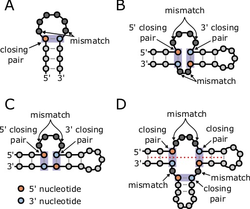
This nearest neighbor model so far only considers the stabilizing energy (negative terms) of a base pair stem, and does not consider the destabilizing energy of structures such as hairpin loops that contributed positive, destabilizing energy to a structure. The Nussinov Algorithm only considers the base pairs, and does not consider that not all basepairs contribute the same energy, as seen in the tables above. Furthermore, it does not take into account the destabilizing energy of the loops, bulges, and other unpaired structures. For example, this image shows some of the common forms of destabilizing energies in RNA structures. Fortunately, there are other algorithms that do compute the minimum free energy including the contribution of these types of structures, and have already been implemented in relatively easy to use software.
The destabilizing energy of a hairpin can be summarized in Table 7.3 [76]. For a loop of length [latex]n[/latex], the destabilizing energy caused by the loop can be approximated by:
[latex]\Delta G_{loop}(n) = 1.75 \times RT \times \ln (n), \label{loopeq}[/latex]
(7.3)
but this equation is only valid for [latex]n \ge 10[/latex]. Other forms of destabilizing energies include hairpin loops, internal loops, bulges, and multiloops (Figure 7.6). In some cases, multiloops can gain stability from coaxial stacking, when two stems on opposite sides of a multiloop share a common axis (Figure 7.6D) [77].
7.4.1 RNAfold
[latex]\texttt{RNAfold}[/latex] is software that comes as part of the Vienna RNA package [79]. To compute a structure for a sequence, simply input the sequence data as a FASTA file using [latex]\texttt{cat}[/latex]. The GNU/Linux program [latex]\texttt{cat}[/latex] simply prints the file to the screen, but upon piping it into a file will run the program. For example, consider the microRNA hairpin sequence for miR-1 in humans:
$ cat mir-1.fasta | RNAfold --noLP -p

>hsa-mir-1-1 MI0000651

UGGGAAACAUACUUCUUUAUAUGCCCAUAUGGACCUGCUAAGCUAUGGAAUGUAAAGAAGUAUGUAUCUCA

(((((.((((((((((((((((..((((((((.....)))...))))).)))))))))))))))).))))) (-29.10)

{((((.((((((((((((((((..((((((((.....))}...))))).)))))))))))))))).))))} [-29.84]

(((((.((((((((((((((((..((((((((.....)))...))))).)))))))))))))))).))))) {-29.10 d=2.64}

frequency of mfe structure in ensemble 0.299677; ensemble diversity 3.99
The result is a prediction of the minimum free energy structure for the molecule (in dot-bracket notation), and the minimum free energy of the structure (in kcal/mol). The dot-bracket notation can be understood as containing matching parentheses that correspond to basepairs. Each left parenthesis has a corresponding right parenthesis, and their positions match which nucleotides are predicted to be paired. Dots correspond to unpaired nucleotides. In addition, by default, two postscript image files are created. The first is a secondary structure image ending in [latex]\texttt{\_ss.ps}[/latex] and the second is a dotplot image ending in [latex]\texttt{\_dp.ps}[/latex]. The resulting image for this sequence is shown in Figure 7.7.
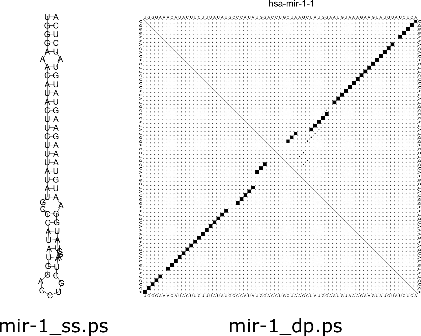
The secondary structure image is a representation of how the structure of the RNA would look in a 2D plane. In a real 3D tertiary structure, there would be helical turns in the stem region of the structure. The dotplot figure shows a matrix where below the main diagonal demonstrates the base pairs present in the minimum free energy structure. Each term of the matrix corresponds to a pair [latex]i,j[/latex] of positions along the sequence. If the two nucleotides at positions [latex]i[/latex] and [latex]j[/latex] are paired, then that cell of the matrix is filled. Above the main diagonal shows the probability of each basepair. You will notice some faint dots around the main larger ones, corresponding to basepairs that could form in suboptimal configurations.
Next, let's consider computing the structure of a tRNA. Suppose that the FASTA file [latex]\texttt{trna.fasta}[/latex] contains a tRNA for the yeast species Saccharomyces cerevisiae. We can compute the structure as before with the command:
$ cat trna.fasta | RNAfold --noLP -p

>Saccharomyces_cerevisiae_chrXVI.trna12-PheGAA (622631-622540) Phe (GAA) 92 bp Sc: 69.79

GCGGAUUUAGCUCAGUUGGGAGAGCGCCAGACUGAAGAAAAAACUUCGGUCAAGUUAUCUGGAGGUCCUGUGUUCGAUCCACAGAAUUCGCA

((((((...((((........))))....((((((((......))))))))......((((..((((........))))..)))))))))). (-30.40)

((((((,..((((........)))),{..((((((((......))))))))..},..{(((..((((........))))..)))))))))). [-31.39]

((((((...((((........))))....((((((((......))))))))......((((..((((........))))..)))))))))). {-30.40 d=3.52}

frequency of mfe structure in ensemble 0.199156; ensemble diversity 5.29
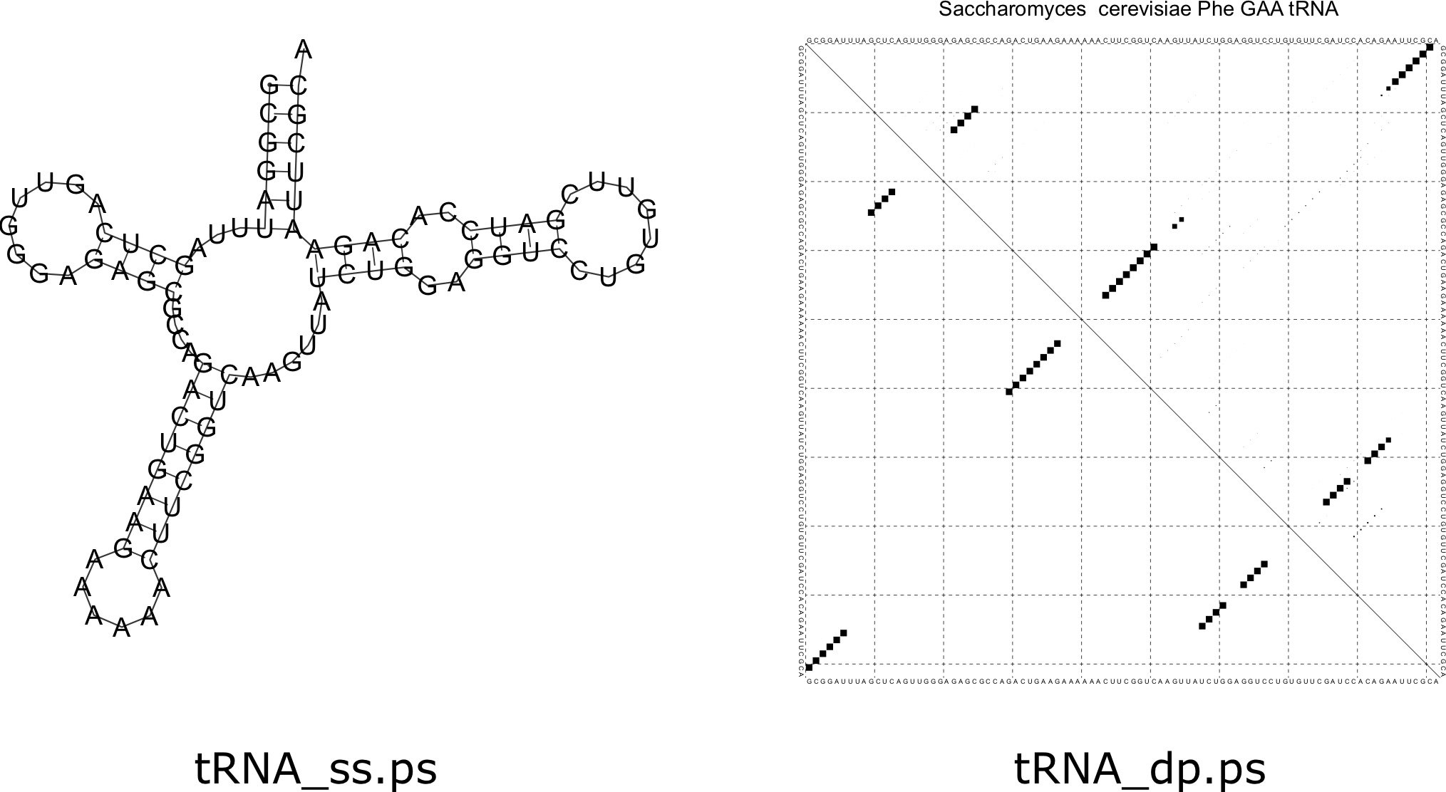
The result is something that looks kind of like a cloverleaf structure. An important fact about tRNAs is that they are chemically modified in the cell, which results in a different structure than one might predict. In the end, the specific structure formed by a tRNA probably looks different than the predictions here due to these modifications. The images produced by [latex]\texttt{RNAfold}[/latex] are depicted in Figure 7.8.
7.5 Lab 8: RNA Structure
7.5.1 RNA Secondary Structure Prediction with RNAfold
Copy and paste the following hairpin sequence to a FASTA file called "hairpin.fasta":
>hairpin

ACAUACUUCUUUAUAUCCAUAUGAACCUGCUAAGCUAUGGAUGUAAAGAAGUAUGU
We can compute the secondary structure of this hairpin with RNAfold:
$ cat hairpin.fasta | RNAfold
Comment on the hairpin structure dot-bracket sequence and the energy (given in parentheses). How big is the hairpin loop in terms of number of nucleotides? How many nucleotides are paired?
7.5.2 RNA Duplex Prediction with RNAduplex
Now let's use RNAduplex to compute the energy of the RNA duplex formed by two RNA strands. Create a FASTA file called [latex]\texttt{arms.fa}[/latex] with the following 5' and 3' "arms" of the hairpin:
>five

ACAUACUUCUUUAUAUCCAUA

>three

UAUGGAUGUAAAGAAGUAUGU
Now compute the duplex energy:
$ cat arms.fasta | RNAduplex
Given the differences in energies between the duplex and the hairpin, How much destabilizing energy would you say the hairpin loop give?
7.5.3 The Destabilizing Energy of a Hairpin Loop
Let's make the calculation of the hairpin loop's destabilizing energy more rigorous. Let's try increasing the length of the hairpin loop by inserting nucleotides to the hairpin loop sequence above in increments of two. Note: You should choose nucleotides that aren't self-complementary to avoid creating more base pairs. Also, check the dot-bracket sequence to make sure that no new base pairs are added.
Make a table with the difference in the hairpin energies and the duplex energies for the different lengths. How does the difference in energy change with the length of the loop? How does this compare to equation 7.3? Try plotting the difference [latex]\Delta \Delta G = \Delta G_{hairpin} - \Delta G_{duplex}[/latex]. This difference should be due in part to the positive energy "cost" associated with the loop.

