2 Measures of Disease Frequency
Learning Objectives
After reading this chapter, you will be able to do the following:
- Define and calculate prevalence
- Classify individuals as either at risk of disease or not
- Define and calculate incidence proportion
- Construct intervals of person-time at risk for a given population
- Define and calculate incidence rate
- Differentiate between incidence and prevalence, and explain the mathematical relationship between them
In public health, we often want to quantify disease—how many people are affected by this health outcome? At first glance, this might seem like a simple question, but once you consider the many applications of quantifying disease, the complexities become apparent. In this chapter, you will learn about 3 measures of disease frequency: counts, prevalence, and incidence.
Counts (a.k.a. Frequencies)
Sometimes, particularly for extremely rare conditions, we only need to know how many people are sick. How many cases of disease X or health behavior Y were there? A count is just a number—there are no fractions, numerators, or denominators, and the units are always “people.”
During the 2017/2018 academic year, for instance, an outbreak of meningococcal meningitis at Oregon State University (OSU) was quantified by counts: 6 students got sick.i
From surveillance data (see chapter 3), we know that the expected number of cases of meningococcal meningitis in a given year is zero. Therefore, 6 cases constitute a level quite above what is expected and would be termed an epidemic (see chapter 3).
For rare conditions like this one, simply knowing how many cases there are is sufficient for a proper public health response. Since we normally expect none, officials at OSU and the local health department just needed to know that there were 6 students with meningococcal meningitis in order to mount a response (in this case, requiring students 25 years old and younger to be vaccinated).i
Similarly, we could look at animal rabies cases observed in Oregon over a 10-year period:
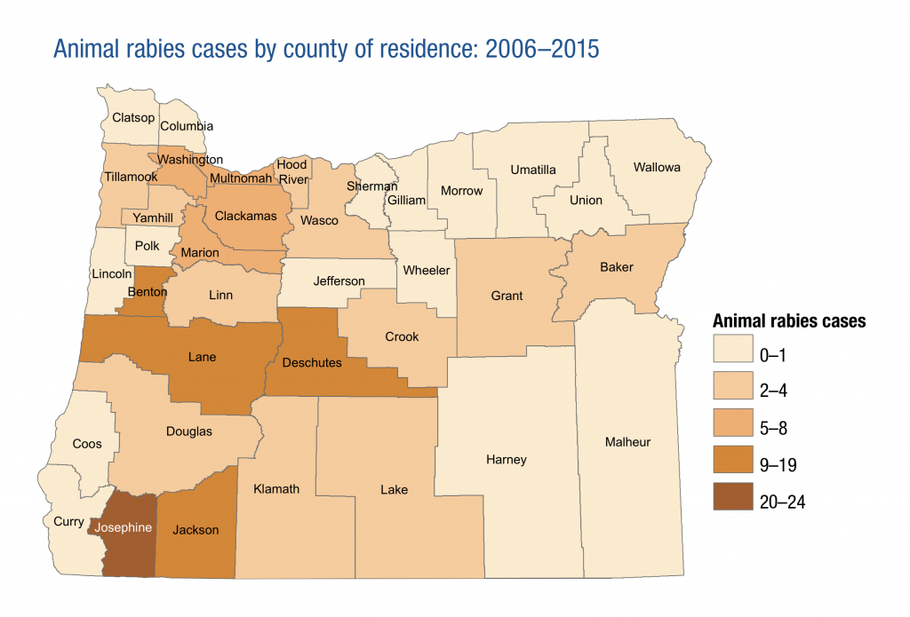
The above picture is useful from a public health infrastructure perspective[1]; if you work at the health department in Josephine County, then you might want to keep a few doses of rabies vaccine on hand (since cases of rabies in animals are often discovered because the infected animal bit a human, who must then be vaccinated). However, if you work at the health department in Wallowa County, which has had no recorded cases of animal rabies in 10 years, then maybe your resources would be better spent on things other than vaccine doses that will likely expire before they are used (assuming you could quickly get doses of the vaccine from the state or neighboring counties if they ever became necessary).
Counts are less useful if we want to compare 2 populations. For instance, 1,000 cases of flu in Ashland, New Hampshire, versus 100,000 cases of flu in New York City—we cannot compare these 2 figures at a glance, because the denominators (i.e., the number of people living in each city) are so different.
Incidence and Prevalence
There are 2 commonly used measures of disease frequency that incorporate denominator information: one is a measure of existing disease (prevalence), and the other is a measure of new disease (incidence). Incidence is used to study causes of disease, whereas prevalence is used more for resource allocation.
Prevalence
Prevalence is a proportion, meaning that everyone who appears in the numerator must also appear in the denominator. This also means that prevalence ranges from zero (no one has the disease) to one (everyone has the disease), and it is usually expressed as a percent.
Prevalence gives us a snapshot of the population-level disease burden at a given time. The formula for prevalence is
Looking at the formula for prevalence, you can see that everyone in the numerator is also in the denominator. Like counts, prevalence is used for resource-planning purposes. Consider the following question a public health authority might be faced with: How much money should our county health department spend on health education about smoking versus on physical activity? One metric for deciding might be which behavior is more prevalent in the local population.[2]
The “at a specified time” part of the prevalence definition could refer either to a specific date (e.g., what was the prevalence of flu in Newport, OR on January 22, 2018?) or to a time point in people’s lives (e.g., what is the prevalence of breastfeeding at 6 weeks postpartum?).
The numerator for prevalence is all current cases. Whether the cases were diagnosed yesterday or 20 years ago doesn’t matter; both would appear in the numerator. Thus prevalence is affected both by the rate at which new cases occur (the incidence, see below) and by how long people typically live with disease. Prevalence is therefore less useful for conditions such as a cold or the flu (where people recover quickly) because once they recover, they are no longer a prevalent case. At any given point in time, most people don’t have the flu, and so it would seem like the disease burden is quite low based on point prevalence, or prevalence calculated on a specific date. In such instances, we sometimes calculate period prevalence instead, which is just prevalence of disease over the course of a longer time frame: for example, what was the prevalence of flu in Newport, OR during the entire 2017-2018 flu season? The numerator here would be all of the cases that occurred at any time during those months (counting only the first instance if anyone was unlucky enough to have influenza twice), and the denominator would be everyone who lived in Newport during those same months.
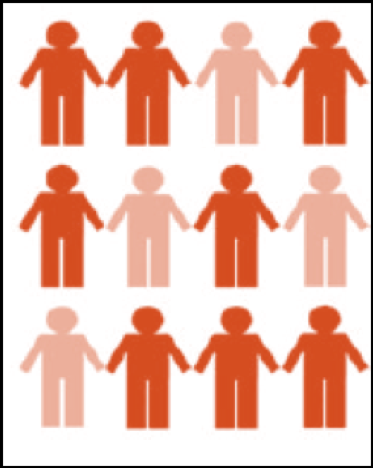
As another example, in Figure 2-2, the prevalence of being light orange is 4/12 = 0.33 = 33%. Note that prevalence does not have units (though providing the specified time is often appropriate and never wrong).
Prevalence Examples
Example 1 (Hypothetical Data)
If there are 5,000 students who live in the dorms at Oregon State University (OSU), and during winter term 2018, 400 of them had the flu at some point, then the prevalence of flu was
400/5,000 = 0.08 = 8.0% of students living in the dorms during winter term 2018 had the flu at some point
The above is an example of a period prevalence, since we were calculating it over a time period longer than one day. It is also an example of the specified time being calendar time—for everyone involved, the specified time was the 2018 winter term.
Example 2 (Based on Known Birth, Infant Death, and Breastfeeding Rates in Oregon)
In 2012, 48,972 babies were born in Oregon. At 14 weeks postpartum, 33,399 of them were being breastfed, and 146 had died. What is the prevalence of breastfeeding at 14 weeks postpartum?
Here we need to subtract the 146 infants who died before 14 weeks from the denominator, as they are no longer part of the population:
33,399/(48,972-146) = 0.684 = 68.4% of infants born in Oregon in 2012 were being breastfed at 14 weeks postpartum
The above is an example of the specified time being a particular point in someone’s life: the day on which a given baby turns 14 weeks old varies depending on the day he or she was born. This is not a period prevalence, because everyone was assessed on one day—we have just spread those days out throughout the year.
Example 3 (Based on National Estimates)
You can also reverse the calculations to establish the number of people with a disease, given the prevalence and population size. In a report on bone health by the Centers for Disease Control and Prevention (CDC),v the authors reported that the prevalence of osteoporosis among men aged 65 and older was 5.6%, and the prevalence among women aged 65 and older was 24.8%. According to data from the US Census Bureau,vi as of July 1, 2017, there were an estimated 22,564,684 men and 28,293,995 women aged 65 and older living in the US. Applying the prevalence, we can estimate that:
22,564,684 × 0.056 = 1,263,622 men aged 65 or older
and
28,293,995 × 0.248 = 7,016,911 women aged 65 or older
currently have osteoporosis in the US.
Incidence
Incidence is a tricky word in epidemiology, because while it is always a measure of new cases, there are 2 possible denominators and at least a half-dozen words that all refer to this same thing. Yikes!
The numerator for incidence is always the number of new cases of a disease observed over some time period. This means that, to study incidence, you must (1) follow people for some length of time (the length varies according to the disease—a few hours or days for a foodborne illness versus a few decades for some cancers) and (2) start with a population at risk—that is, people who are at risk of developing the disease (at risk of becoming a case). Usually, at a minimum, we therefore exclude people who already have the disease—such people cannot become an incident case because they are already a prevalent case. We also exclude anyone not capable of getting the disease, either because they are immune or because they lack the proper organs (e.g., biological females cannot get testicular cancer). Furthermore, because you are establishing the number of new cases, it is always necessary to include time-based units when reporting an incidence.
One way of calculating incidence is to include in the denominator the number of people who were at risk of getting the condition at the start of your follow-up time period. This calculation yields the incidence proportion. It’s also called, depending on which source you’re reading, the cumulative incidence, or the risk.[vii]
The incidence proportion is interpreted as the average risk (chance) of developing the disease over some time period.
Incidence examples
Example 1 (Hypothetical Data)
If there are 25 students in a particular class, and one person came to class on Monday of the first week already sick with the flu (this person is a prevalent case—they are already sick, so are not at risk), and 2 more people got the flu on Wednesday of that same week, then what was the incidence of flu during Week 1?
Our numerator would be the number of new cases of flu—here, 2. The denominator is the population at risk, so we must subtract out the student who already has the flu because they are not at risk. So the denominator is 24.
The incidence of flu in that class during Week 1 was thus:
2/24 = 0.083 = 8.3 per 100 per week
Although prevalence is usually expressed as a percent, for incidence we use “per 100,” “per 1,000,” “per 10,000,” and so on. The precise power of 10 is not standardized; just choose one that gives you a whole(ish) number of people: 8.3 per 100 is the same as 83 per 1,000.
Additionally, it is vital that you specify the time period over which you observed incidence, because interpretation (e.g., how much of a problem this particular disease is) varies widely depending on time. For instance, 2 cases of breast cancer per 100 women in one week are very different than 2 cases per 100 women in 20 years. The former might warrant public health intervention, while the latter almost certainly would not.
Example 2 (Hypothetical Data)
If we want to compare the incidences between 2 populations, it is important to express them in the same power of 10 (e.g., both must be “per 100” or “per 1,000”) and also to convert them to cover the same time frame.[3]
If City A has an incidence of norovirus of 25/1,000 per month and City B has an incidence of norovirus of 500/10,000 per year, we cannot compare them. We must first convert one of the denominators and one of the time frames so that they are comparable.
Here we’ll convert the numbers for City A. First, the denominator needs to be 10,000, not 1000. If we multiply the incidence for City A by 10/10,[4] the incidence in City A is now 250/10,000 per month.
Then we need to adjust the time frame—here by multiplying by 12 (as there are 12 months in a year). The incidence in City A then becomes:
250 × 12 = 3000/10,000 per year
Compared to City B’s incidence of 500/10,000 per year, the incidence is higher in City A.
Some of you will have spotted a potentially questionable assumption made above: that the incidence in City A—which was measured only over one month—is constant for the entire year. This may or may not actually be true, and in real life, you would have to do a little digging to determine whether it was likely true or not before declaring that norovirus was more common in City A. What if the 1-month data point was from an anomalous month, when City A had a huge norovirus outbreak, for instance? This is not uncommon, because like flu, norovirus is seasonal.
We have thus far been looking at incidences with a relatively straightforward population calculation—for example, the number of students living in a particular dorm at a particular time. The other kind of incidence is the incidence rate. Some epidemiology texts will call this the incidence density.[vii] Importantly, the numerator is still the number of new cases observed over a given period of time. But the denominator is now the sum of the person-time at risk.
The need for this “other” kind of incidence stems from the fact that populations are not static: some people are born, others die, people move in and out. Thus if you quantify the population at risk at the start of your observation window, you are at best only approximating the population, particularly if you follow people for a year or more. Instead, we could look at each person in the population and determine how long they were at risk. Figure 2-3 shows a hypothetical population with 10 people, all of whom were at risk at the start of a 1-year follow-up observation period:
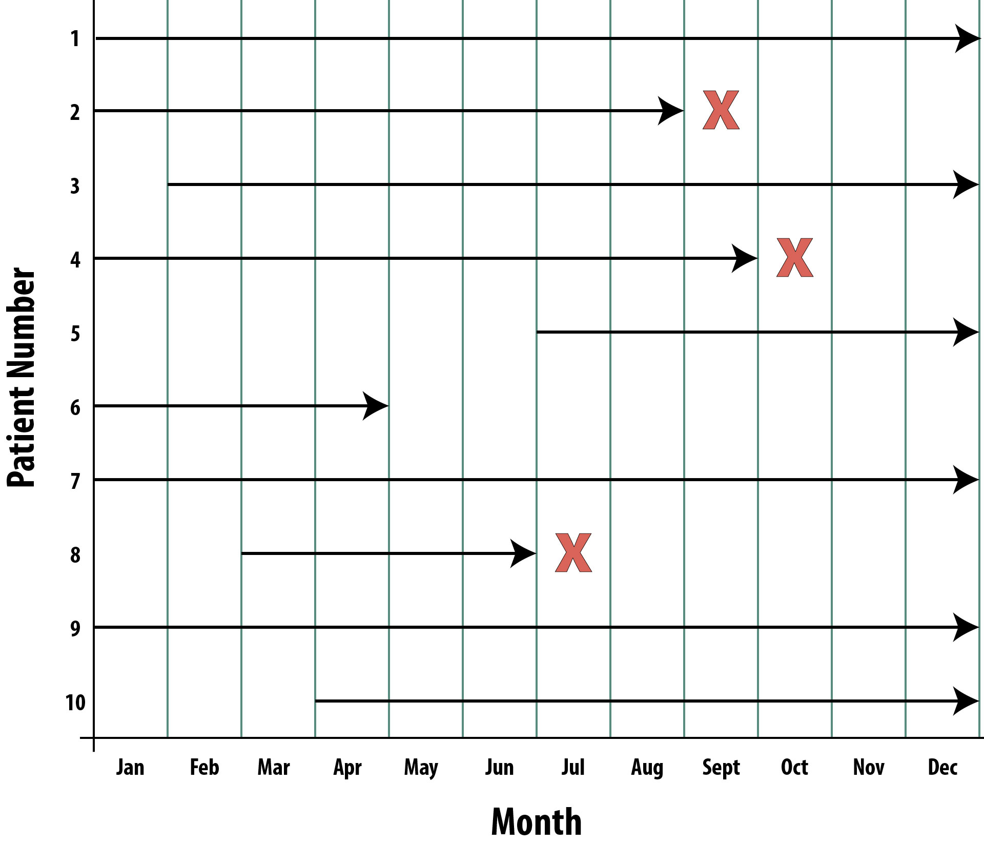
Person 1 enrolled in the study January 1 and was followed through December 31 without developing the disease of interest (they may have been diagnosed with other things, but if they have not contracted the disease we’re studying, then they’re still at risk). Person 1 contributed 12 person-months at risk.
Person 2 enrolled January 1 and developed the disease at the end of August. Person 2 contributed 8 person-months at risk. Person 2 is still alive after August but can no longer contribute person-time at risk because now they are a prevalent case.
Person 3 didn’t enroll until February 1 and was then followed for the rest of the year without developing the disease of interest. Person 3 contributed 11 person-months at risk.
Person 4 enrolled January 1 and developed the disease at the end of September. Person 4 contributed 9 person-months at risk.
Person 5 enrolled July 1 and did not develop the disease during follow-up. Person 5 contributed 6 person-months at risk.
Person 6 enrolled January 1 and was lost to follow-up at the end of April (this person could have moved away, stopped returning calls, or maybe died of something else—these are called competing risks). Person 6 contributed 4 person-months at risk. We can still count these months, because during that time, Person 6 was in the study, and was still at risk—not knowing the outcome (if they moved, etc.) or having their follow-up terminated because of death from a competing risk does not negate the fact that we observed Person 6 for 4 months while they were at risk.
Person 7 enrolled January 1 and was followed through December 31 without developing the disease under investigation. Person 7 contributed 12 person-months at risk.
Person 8 enrolled March 1 and developed the disease at the end of June. Person 8 contributed 4 person-months at risk.
Person 9 enrolled in the study January 1 and was followed through December 31 without incident. Person 9 contributed 12 person-months at risk.
Person 10 enrolled in the study April 1 and was followed through December 31 without incident. Person 10 contributed 9 person-months at risk.
To calculate the incidence rate, then, our numerator is still the number of new cases we observed during the follow-up time—here, there were 3 new cases (persons 2, 4, and 8). The denominator is now the sum, in months, of the person-time at risk contributed by all participants.
Calculating Incidence Rate from Data in Figure 2-3
First sum the total person time at risk:
12 + 8 + 11 + 9 + 6 + 4 + 12 + 4 + 12 + 9 = 87 person-months at risk (PMAR)
Then calculate the incidence rate:
3/87 PMAR = 0.0345 per person-month (PM)
That looks a little ugly, so let’s move the decimal place:
3.45 per 100 person-months
We could instead express this in terms of years by multiplying our original by 12 (because there are 12 months in the year):
(0.0345 per PM)(12) = 0.414 per person-year
Finally, we could make it have at least one whole person:
4.14 per 10 person-years
In other words, in Figure 2-3, we observed 4.14 new cases of disease for every observed 10 person-years at risk.
The strengths of the person-time approach are that it allows a more nuanced view of the population at risk and is more realistic: not everyone enrolls in a study on exactly day one, some people experience competing risks or are lost to follow-up, and sometimes a case pops up almost immediately, so that person contributes very little person-time to the denominator (whereas with incidence proportion, they would add a full person).
Limitations of the person-time approach are that it is more complex, and it does not distinguish between 100 people followed for one month (totaling 100 PM), 10 people followed for 10 months (totaling 100 PM), and one person followed for 100 months (still totaling 100 PM). Additionally, loss to follow-up is probably not random (this could also affect incidence proportion if people drop out because they’re feeling poorly but before they are recorded as an incident case). It is thus useful to state the time-period over which people were eligible to be followed (in Figure 2-3, one year). Table 2-1 compares the two types of incidence.
| Incidence Proportion | Incidence Rate | |
| Numerator | new cases over a period of time | new cases over a period of time |
| Denominator | number of people at risk at the start | sum of person-time at risk |
| You must: | define the time frame | report the person-time units |
| A.K.A. | risk cumulative incidence absolute risk |
incidence density |
| Range | 0-1 (it’s a proportion)[5] | 0 to infinity |
Prior Person-Time at Risk
What about all that time before our study started? If we enroll a bunch of 50 year-olds who are at risk of heart disease and follow them recording the person-time, why not also count the person-time at risk from prior to study entry? Each person would yield an extra 50 years of person-time at risk!
We can’t do this because we are missing all of the prevalent cases. Some proportion of people develop heart disease prior to age 50, and would thus not be eligible for our study. Without data on how many person-years at risk those people had prior to developing heart disease, our incidence would be artificially low, because we add 50 person-years at risk per person to the denominator without accounting for the entire population, which includes some cases that are prevalent by age 50.
Uses of Incidence and Prevalence
As stated above, incidence is used to study the causes of disease. Prevalence is less useful for this because the disease has already happened; we thus have no way of knowing whether the disease or the exposure happened first (necessary for establishing causality). For instance, obesity is associated with lower levels of physical activity—one possible scenario is that lower levels of physical activity lead to obesity, secondary to an energy imbalance. However, another equally possible scenario is that obesity came first and the person subsequently reduced their amount of physical activity, possibly secondary to joint pain. Studying prevalent obesity cases does not allow us to distinguish between these scenarios.
Incidence, on the other hand, can easily be used to study potential causes of disease. When studying incidence, we know that everyone is disease-free at baseline, since we study only the population at risk. Therefore, any exposures assessed at the beginning came before disease onset by definition.
Prevalence is more useful as a way of assessing the disease burden in a particular community, perhaps for purposes of resource allocation. For instance, state health departments in the Northeast and upper-Midwest spend a portion of their budgets on Lyme disease prevention education (e.g., billboards about tucking your pants into your socks) because Lyme disease is quite prevalent in those regions:
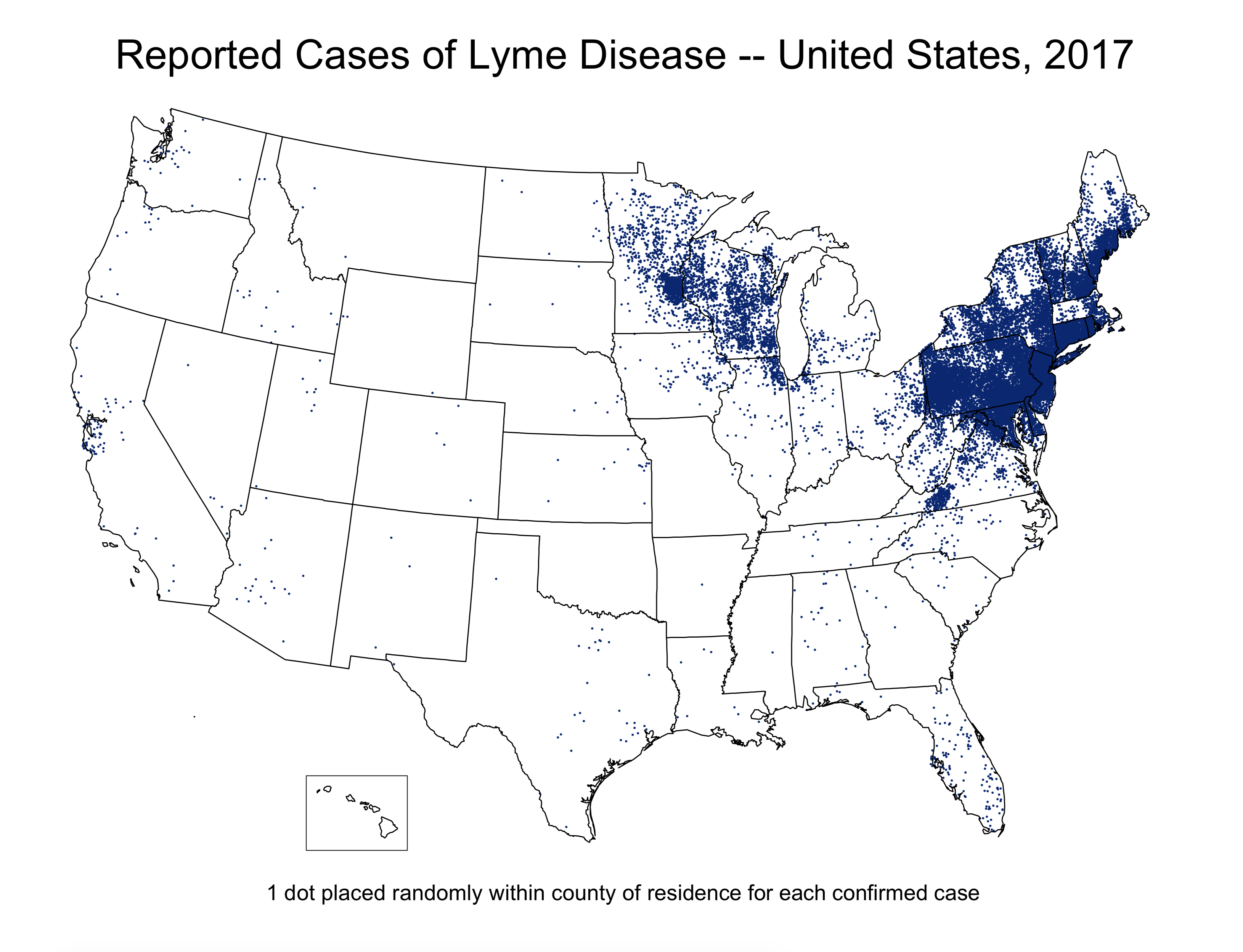
Source: https://www.cdc.gov/…/maps.html
However, the prevalence of Lyme disease in Colorado is extremely low; health departments in Colorado would do well to spend their money elsewhere. Prevalence data are also useful for health care administrators: if you know that 80% of your nursing home residents have dementia in some form, then this has implications for staffing, standard operating procedures, and potentially even for the layout and design of the space (pictorial signs on the walls to indicate the purposes of rooms, for instance).
Relationship between Incidence and Prevalence
As mentioned above, prevalence is affected by both the incidence (how many new cases pop up) and the disease’s duration. If people live longer with a disease, then they remain prevalent cases for longer. Thus
Here is an example:
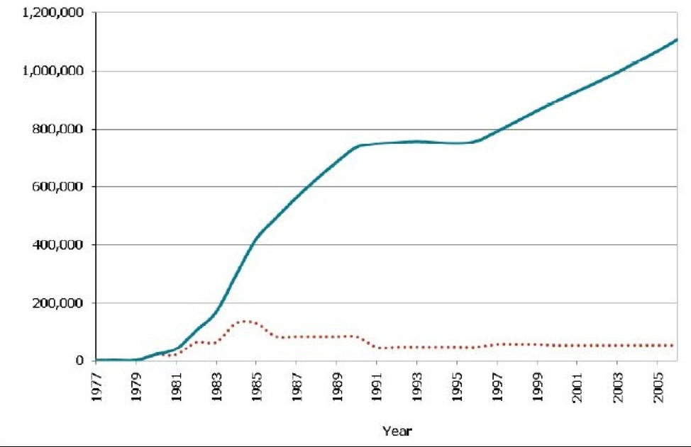
Source: CDC Fact Sheet HIV in the United States, July 2010
Figure 2-5 shows the prevalence (blue line) and incidence (red dotted line) of HIV. In the early 1980s at the beginning of this epidemic, before we knew what caused AIDS and before we knew that condom use, screening blood donations, and universal precautions by health care personnel could prevent the spread of the virus, the incidence kept going up. More people got infected, and then they in turn infected others. However, we also could not treat HIV initially, and so people would die of AIDS within a few years. The early rise in prevalence is thus attributable solely to the rising incidence. Then we discovered how to prevent new cases: thus, the incidence went down, and while the prevalence took a couple years to catch up, it eventually leveled off. In 1996, access to highly active antiretroviral treatments (HAART) became common,[viii] and it was now possible for people to “live with HIV.” The increasing prevalence, starting in the late 1990s, is thus due entirely to an increase in patient survival, or the average duration of illness (you can see that the incidence is steady at that time).
Prevalence therefore comprises 2 characteristics of a disease within a population: the incidence and the average survival time. A change in either one of these components would lead to a change in prevalence; thus, when a change in prevalence is observed, the smart public health professional pauses to consider whether the change is due to a change in the number of new cases (incidence) or to a change in available treatments (and thus survival). One can see that a public health department’s response to each of these scenarios would be different.
Summary
This chapter discusses 3 measures of disease frequency: counts, which are used for extremely rare conditions; prevalence, which considers new and existing cases and is used for resource allocation; and incidence, which considers only new cases and is used to study disease etiology.
Incidence can further be broken down into incidence proportion (which uses the number of people at risk as the denominator) and the incidence rate (which uses the sum of the person-time at risk as the denominator). Prevalence is approximately equal to the incidence multiplied by the average survival time after diagnosis.
References
i. Meningococcal disease. Student Health Services. 2009. https://studenthealth.oregonstate.edu/infectious-diseases/meningococcal-disease. Published August 28, 2009. Accessed October 19, 2018. (↵ Return 1) (↵ Return 2)
ii. Oregon Health Authority . Oregon birth data. State of Oregon. https://www.oregon.gov/oha/PH/BirthDeathCertificates/VitalStatistics/birth/Pages/index.aspx. Accessed October 19, 2018.
iii. Oregon Health Authority . Deaths and perinatal deaths data : Annual report volume 2 : State of Oregon. https://www.oregon.gov/oha/PH/BIRTHDEATHCERTIFICATES/VITALSTATISTICS/ANNUALREPORTS/VOLUME2/Pages/index.aspx. Accessed October 19, 2018.
iv. Breastfeeding report card, United States, 2013. Centers for Disease Control and Prevention (CDC). 2013. http://www.cdc.gov/breastfeeding/data/reportcard.htm. Accessed September 5, 2014.
v. Percentage of adults aged 65 and over with osteoporosis or low bone mass at the femur neck or lumbar spine: United States, 2005–2010. CDC. https://www.cdc.gov/nchs/data/hestat/osteoporsis/osteoporosis2005_2010.htm. Accessed July 31, 2018. (↵ Return)
vi. American FactFinder—results. Bureau USC. https://factfinder.census.gov/faces/tableservices/jsf/pages/productview.xhtml?pid=PEP_2015_PEPAGESEX&prodType=table. Accessed July 31, 2018. (↵ Return)
vii. Last JM. A Dictionary of Epidemiology. 4th ed. New York: Oxford University Press. (↵ Return 1) (↵ Return 2)
viii. Byrne M. A brief history of AZT, HIV’s first “ray of hope.” Motherboard. 2015. https://motherboard.vice.com/en_us/article/mgb48x/happy-birthday-to-azt-the-first-effective-hiv-treatment. Accessed October 19, 2018. (↵ Return)
- The final line in the 'Animal rabies cases' key has been edited to read '20-24.' The original source image reads '2-24.' ↵
- We would use counts to make these decisions when the condition in question is extremely rare, such that the prevalence would be 0.000001% or similar. Then denominators are not as important—this is the case for rabies, as discussed above. ↵
- We don’t need to worry about population size, because the incidence calculation accounts for those denominators. ↵
- Recall from your Algebra classes that this is a legal maneuver, because 10/10 = 1, and you can multiply numbers by 1 with impunity. ↵
- if the numerator is the number of cases of a disease that you can get more than once, then incidence proportion can be above 1, because the denominator is still people. For this reason, usually we count only the first episode of a given disease. ↵
Quantifies how much disease is in a population. See count, incidence, and prevalence.
A measure of disease frequency used in lieu of prevalence when the disease is extremely rare.
A measure of disease frequency that quantifies existing cases. The numerator is "all cases" and the denominator is "the number of people in the population." Usually expressed as a percent unless the prevalence is quite low, in which case write it as "per 1000" or "per 10,000" or similar. There are no units for prevalence, though it is understood that the number refers to a particular point in time.
A measure of disease frequency that quantifies occurrence of new disease. There are two types, incidence proportion and incidence rate. Both of these have “number of new cases” as the numerator; both can be referred to as just “incidence.” Both must include time in the units, either actual time or person-time. Also called absolute risk.
The ongoing, systematic collection, analysis, and interpretation of health data, essential to the planning, implementation, and evaluation of public health practice, closely integrated with the timely dissemination to those who need to know. Surveillance both (1) provides information for descriptive epidemiology (person, place, time), and (2) allows us to know what "normal" is, so that potential epidemics are identified early. Also called public health surveillance.
The occurrence, in a community or region, of cases of an illness (or specific health-related behaviour or other health-related events) clearly in excess of normal expectancy. Epidemiologists and other public health professionals keep track of what levels are "expected" through surveillance.
After birth.
Prevalence calculated at a specific moment in time.
Prevalence calculated over a longer period of time. Used for short-duration infectious diseases or injuries.
All individuals in a population who (1) have not yet experienced the disease or health outcome under study; and (2) are capable of experiencing that disease or health outcome. In other words, the population at risk excludes all prevalent cases, as well as those who for some reason could never experience the outcome (eg, biological males cannot have endometrial cancer). It is not always possible to correctly identify those in the latter group, depending on the disease or health outcome in question. For instance, technically, if we were studying pregnancy, we would need to exclude all women who are either themselves infertile or who are in a monogamous relationship with a man who is infertile. However, in practice it is difficult to identify infertile couples (those who have never tried to get pregnant won't know they're infertile); in such a scenario one would just acknowledge the limitation (that the calculation of population at risk was imperfect, and why).
A measure of disease frequency. The numerator is "number of new case" and the denominator is "the number of people who were at risk at the start of follow-up." Sometimes if the denominator is unknown, you can substitute the population at the mid-point of follow-up (an example would be the incidence of ovarian cancer in Oregon. We would know how many new cases popped up in a given year, via cancer surveillance systems. To estimate the incidence proportion, we could divide by the number of women living in Oregon on July 1 of that year. This of course is only an estimate of the true incidence proportion, as we don't know exactly how many women lived here, nor do we know which of them might not have been at risk of ovarian cancer.) The units for incidence proportion are "per unit time." You can adjust this if necessary (ie if you follow people for 1 month, you can multiply by 12 to estimate the incidence for 1 year). You can (read: should) also adjust the final answer so that it looks "nice." For instance, 13.6/100,000 in 1 year is easier to comprehend than 0.000136 in 1 year. Also called risk and cumulative incidence.
See Incidence Proportion.
See Incidence Proportion.
A measure of disease frequency. The numerator is "number of new cases." The denominator is "sum of the person-time at risk." The units for incidence rate are "per person-[time unit]", usually but not always person-years. You can (and should) adjust the final answer so that it looks "nice." For instance, instead of 3.75/297 person-years, write 12.6 per 1000 person-years. Also called incidence density.
See incidence rate.
For participants enrolled in a cohort study or randomized controlled trial, this is the amount of time each person spent at risk of the disease or health outcome. A person stops accumulating person-time at risk (usually shortened to just "person-time") when: (1) they are lost to follow-up; (2) they die (or otherwise not become a risk) of something else other than the disease under study (ie they die of a competing risk); (3) they experience the disease or health outcome under study (now they are an incident case); or (4) the study ends. Each person enrolled in such a study could accumulate a different amount of person-time at risk.
In a cohort study or randomized controlled trial, competing risks are defined as “everything else that might kill someone or otherwise make them no longer at risk of the outcome under study.” So, if we are studying ovarian cancer, then possible competing risks are fatal motor vehicle accidents, fatal heart attacks, etc., as well as oophorectomy (surgical removal of the ovaries). If someone experiences a competing risk, they no longer contribute person-time at risk.
A chronic, arthritis-like disease spread through tick bites. Endemic in parts of the US.
The sum of what is known about how a disease process develops within an individual, including known determinants.
