Human-Altered Systems
7 Agroecosystems
How Does Agriculture Influence the Earth System? How Can We Reduce Its Negative Impacts?
The year is heavy with produce. And the men are proud, for of their knowledge they can make the year heavy. They have transformed the world with their knowledge.
—John Steinbeck, The Grapes of Wrath
On the western edge of North America, hemmed in by some of its tallest mountains, lies the most productive farmland on Earth: the Great Central Valley of California. The statistics of its bounty are impressive, if a bit abstract. Although it comprises less than 1% of US farmland, the region produces one-quarter of the nation’s food. That includes more than 250 different crops that range from commodity staples such as wheat to the avocados we spread on toast. It is the primary or sole producer of many of the nation’s fruits and nuts, such as almonds, pistachios, walnuts, and peaches.1 All that production is the main reason why California is the nation’s richest agricultural region by a wide margin. In 2020, the state’s producers generated $50.1 billion in sales.2
It has always been a biologically productive place, the result of a fortunate convergence of rich alluvial soils, a mild sun-drenched climate, and, at least for part of the year, abundant water. Since our first arrival in the valley, we have worked to channel that productivity into food. Initially, one of our main tools was fire, which we used to promote open oak savanna that included oaks as well as a diversity of grasses and forbs. Indigenous communities throughout the valley combined the fire management with more nuanced husbandry of the specific plant species they valued for food, sources of medicine, and as manufacturing materials. The grasslands and wetlands in turn supported abundant game species such as pronghorn (Antilocapra americana), elk (Cervus canadensis), and waterfowl.3 When John Muir described this oak savanna in the mid 1800s, he was awed by its wildflowers and their potential to make honey, although he was largely oblivious to the fact that it was partly a designed creation of the region’s Indigenous people:4
The Great Central Plain of California, during the months of March, April, and May, was one smooth, continuous bed of honey-bloom, so marvelously rich that, in walking from one end of it to the other, a distance of more than 400 miles, your foot would press about a hundred flowers at every step. Mints, gilias, nemophilas, castilleias, and innumerable compositæ were so crowded together that, had ninety-nine per cent of them been taken away, the plain would still have seemed to any but Californians extravagantly flowery.5
Later on, as European settlers poured into the valley, the focus turned to controlling water. As we started to farm domesticated crops sold as commodities, we realized there was one flaw in the otherwise elysian abundance of California: it rained at absolutely the wrong time. Under its Mediterranean-type climate, almost all the precipitation falls during the winter, at least in those happy years when it does fall. This makes farming a crop like winter wheat a perennial gamble, and most of the other 250 crops now grown in the valley a near impossibility. The unique geography of the valley provided a workaround, however. The mountains that rim the valley trap and hold precipitation. In the tallest parts of the ranges, the water is stored as prodigious amounts of snow. This trapped precipitation gets gradually released to the valley as it melts and runs down streams and rivers or percolates through aquifers.
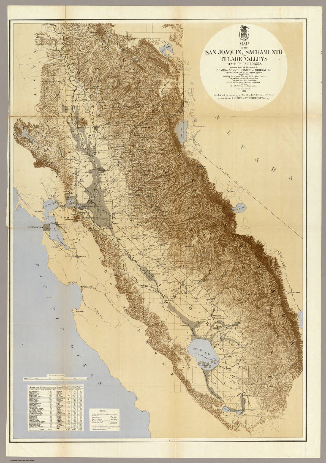
That water used to create one of the world’s greatest ephemeral wetlands. For a few months each spring and early summer, snowmelt created a soggy network of rivers, wetlands, tule swamps, boggy ground, and wet spots that stretched from the base of the Klamath Mountains in the north to the Tehachapi Mountains in the south (Figure 7.1). The great focal points of all this water were the deltas of the Sacramento and San Joaquin Rivers as they converged and drained into San Francisco Bay and Tulare Lake at the far southern end of the valley. In particularly wet years, the two vast wetlands essentially merged. In 1868, a 16-foot scow made the only known successful commercial navigation of the wetlands, traveling from the north fork of the Kings River to San Francisco Bay carrying a load of famed Central Valley honey.6
We realized that if we could harness the pace, timing, and direction of the annual floodwaters, we could grow crops under months of otherwise near-ideal conditions in some of the most fertile soil on the planet. Our initial attempts at bending the elemental force of water to our will were, like many a gold rush grub stake, utter failures. In the neighboring Imperial Valley to the south, the spring floodwaters of 1905 tore through construction work on an irrigation canal, allowing water from the Colorado River to rush into the dry Salton Sea basin for 18 months, creating by farcical accident one of the largest lakes in the country. But by sheer bullheaded persistence at first and later by the technological force of agro-industrialization, we progressively began to wrangle the waters. We diked and drained the wetlands of the Sacramento-San Joaquin Delta and Tulare Lake, we channelized the main rivers flowing through the valley floor, we built dams along the feeder rivers coming from the mountains, and we connected everything into a vast network of aqueducts and irrigation canals. Today, nearly every drop of water that flows through the valley is under our control. Lake Tulare, which had been the largest freshwater lake west of the Mississippi, is now one of the world’s largest privately held farms. The J. G. Boswell Company farms about 60,700 hectares (about 150,000 acres) of the former lake bottom—down a bit from its peak of 80,900 hectares. When Mark Arax and Rick Wartzman toured the farm with J. G. Boswell II in 1999, they drove half the day and covered 150 miles without ever leaving the farm.7
Recent changes to the valley have gone far beyond water. Nearly every aspect of the valley’s biology is now under our direct or indirect influence. About 71% of its land is being intensively farmed at any given time, and another 10% has been converted to towns and cities. The bits that support the flowers of Muir’s honey bloom are now vanishingly small. Less than 15% of the valley is grassland or shrubland, and 2% is wetland.8
The Central Valley of California is like a piece of Anthropocene performance art. In an intense and exaggerated way, it embodies many of the traits and characteristics of how we farm and how we transform the planet. While we derive immense social benefit from farming, it also directly threatens our own well-being. Reconciling that conundrum in ways that equitably distribute the benefits and costs is one of our fundamental challenges (see Figs. 1.17 and 1.18). In this chapter, I explore this challenge from an ecological perspective. I summarize the main ways that agroecosystems influence the Earth System and explore approaches for mitigating their impact while maintaining the ecological services they provide. I won’t explore in any comprehensive way the social or economic aspects that are deeply intertwined with the ecological ones. Many of those social-ecological interactions manifest themselves in the form of profound inequities in things such as access to nutritious food, exposure to toxic chemicals, and opportunities for happiness. I won’t comprehensively explore those either. But I will occasionally bring up a few reminders that we need to consider those aspects of our food system, just as much as the ecological impacts.
7.1 The Diversity of Farming
Section 7.1: The Diversity of Farming
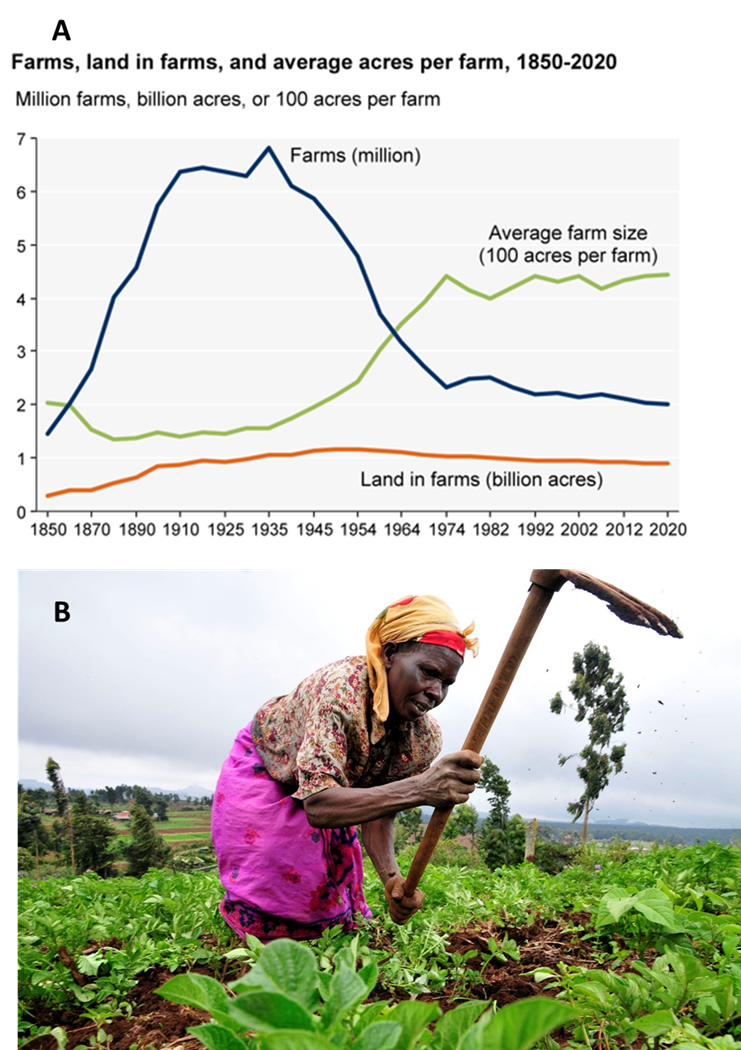
The J. G. Boswell Company farm is extreme, but it isn’t an anomaly. Down the road (so to speak), Stuart Resnick is the world’s largest grower of pistachios, almonds, and pomegranates. He—or rather an umbrella holding company—farms about 52,600 hectares in the Central Valley. Before getting into farming, Resnick built a Los Angeles janitorial business and bought the Franklin Mint (of Civil War and Princess Diana commemorative dishware fame). The POM Wonderful brand of pomegranate juice was his wife’s idea. They also grow those ubiquitous bags of Halos-branded mandarins, and as a side project own the Fiji brand of bottled water.9 In many regions, social and economic factors have driven farms to get larger and to become run as integrated businesses with deep connections to global trade and capital markets. These trends have been most pronounced in the United States (7.2A), South America, and Australia. Contributing factors to the trends include technological innovations that reduce labor requirements and that create significant scale efficiencies, rising land costs, rising nonfarm wages and opportunities, and government policies that favor (both intentionally and unintentionally) larger farms.
Despite their increasing influence, however, these types of farms are just one aspect of our global food system. Estimates range considerably, but as much as 40% of the world’s farms are small operations of less than 2 ha.10 These small family farms (sometimes called smallholder farms) produce more than 75% of the major food commodities in sub-Saharan Africa, Southeast Asia, South Asia, and China (Fig. 7.2B). Globally, small and medium farms (≤50 ha) produce the majority of nearly all the major food commodities and the nutrients we consume.11
More broadly, we farm across a bewildering range of economic, social, and political contexts that have produced an equally varied range of ways that farms are economically structured and interact with political economies. On top of all that, there are about as many ways to farm as there are farmers, and no shortage of opinions about the relative merits of different approaches and practices. Even deciding who a farmer is can be contentious. A Mongolian herdsman or an Oregonian forester might bristle at being called a farmer. Even J. G. Boswell considered himself more a chief executive than a farmer: “No. I got no interest in farming. I never had the time. I was too busy building, growing, perfecting, getting the right people in the right spots.”12 The list of species we farm is similarly varied. We commonly grow roughly 350 plant species for our own direct consumption in addition to the range of species we mainly feed to animals, use for fiber, or for recreation and enjoyment. The list of animals we farm includes the usual barnyard residents, but also a diverse array of aquatic species and even insects.13 We farm in almost every environment on the planet, including Antarctica.14
Crops and Practices
We commonly classify farming systems by what and how we farm. These classifications are useful for helping to develop policy and regulations, estimate economic impacts, and simply make shopping decisions. But crop- and practice-based classifications are problematic as ecological descriptors, particularly for classifications based on the type of crop. For example, the nomadic cattle husbandry systems of Mongolia are different ecosystems than the mechanized feedlots of the Central Valley of California. Similarly, you might be hard pressed to find the ecological commonalities between a subsistence maize plot in the highlands of central Mexico and an Iowa corn field.
Classification systems based on farming practices provide a lot more information about ecological conditions. That is because practices such as the type and amount of fertilizer we apply, how we manage pests, how frequently we till the soil, and whether we irrigate profoundly influence the physical and biological characteristics of agroecosystems. We have developed a wide range of practice-based classifications. Just a few examples include organic, biodynamic, permaculture, conventional, industrial, intensive, extensive, subsistence. Although they are better, these classifications are still not perfect ecological descriptors, partly because there can be a lot of variability in the specific practices that farmers use even within a broad category. That variation often relates to the different environmental, economic, and social constraints that farmers face. For example, the US Department of Agriculture broadly defines organic agriculture in the following way:15
- Use of cover crops, green manures, animal manures, and crop rotations to fertilize the soil, maximize biological activity, and maintain long-term soil health.
- Use of biological control, crop rotations, and other techniques to manage weeds, insects, and diseases.
- An emphasis on biodiversity of the agricultural system and the surrounding environment.
- Using rotational grazing and mixed forage pastures for livestock operations and alternative health care for animal well-being.
- Reduction of external and off-farm inputs and elimination of synthetic pesticides and fertilizers and other materials, such as hormones and antibiotics.
- A focus on renewable resources, soil and water conservation, and management practices that restore, maintain, and enhance ecological balance.
This seems like a specific definition, but there is enough ambiguity and wiggle room in those prescriptions that different farms could fit under them. For instance, the organic label could apply to a smallholder cotton farm in India where all of the labor is provided by family members and draft animals, all the nutrients come primarily from the local production of manure and cover crops, and the water is provided by rainfall. But it could also apply to a mega corporate cotton farm where most of the labor is mechanized and uses fossil fuels, some of the nutrients are sourced from wild-caught marine resources, and the water comes from irrigation. Those two types of farms likely have many ecological differences even though they broadly fall under the same organic classification.
In addition, many practice-based groupings are not explicitly organized with respect to ecological characteristics. They may instead be organized for social, philosophical, ethical, or economic reasons. For instance, the practices associated with cage-free animal husbandry are primarily designed around ethical considerations for how animals should be treated and the quality of the lives they should have while in our service. Some of these practices do indirectly influence how cage-free production systems function as ecosystems but not in a coherent or consistent way.
Finally, individual farms often don’t easily fit into broad stereotypes. Farmers may blend practices from different categories or adaptively vary their practices depending on shifting conditions. For instance, a farmer might mostly follow organic practices but on rare occasions sparingly use a chemical pesticide to combat a severe pest outbreak. Strictly, such a farm would be classified as conventional or non-organic, but it likely has ecological characteristics that are more similar to organic farms than to other conventional farms that chronically use chemical pesticides and fertilizers.
Ecological Metrics and Indicators
So, if the type of crop and overly broad practice-based classifications are insufficient to describe the ecology of farming systems, what is a better way of describing them? One approach is to directly describe the characteristics of agroecosystems using the same ecological metrics that we have developed for ecosystems in general. These can include but are by no means limited to biodiversity metrics such as species richness or functional diversity, ecological processes such as net primary productivity or nutrient cycling, and ecosystem services such as food production or climate regulation. An issue with this approach is that there are a whole lot of potential ecological metrics that we could measure and scales over which we could measure them. It’s hard enough just measuring a few of them, let alone measuring enough to build a comprehensive picture. On top of that, it is often not obvious what specific metrics are needed to answer a specific question or which metrics are most useful in a given context.
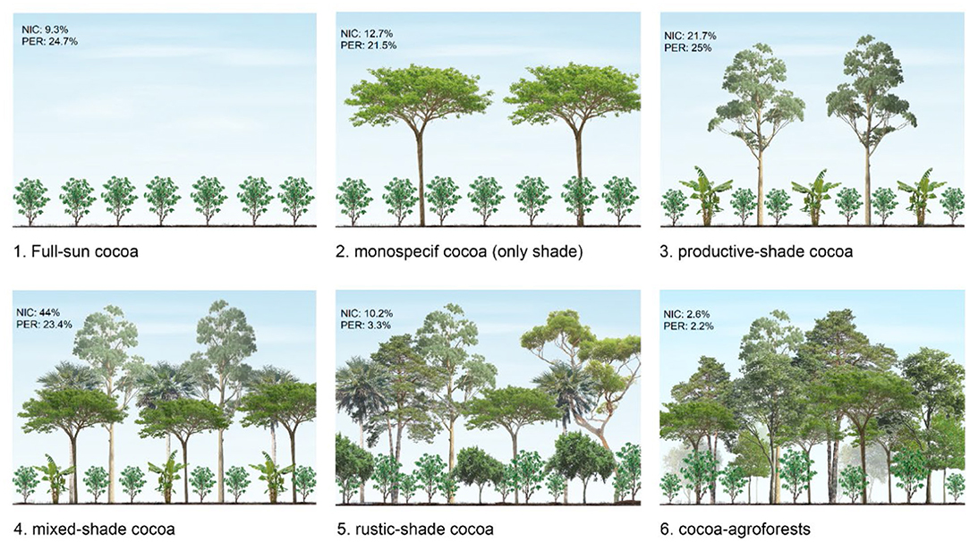
One way that we have addressed this problem is by developing indicator metrics that are associated with a broad syndrome of conditions. For example, indicator species are species whose presence or abundance in a location is associated with particular physical conditions, associations of other species, or types and levels of ecosystem processes. The best indicators are ones that are relatively easy to measure and that are consistently associated with other more difficult-to-measure attributes. An example comes from cacao (Theobroma cacao), or cocoa as the processed products are confusingly called. Global cacao production has more than doubled over the past 50 years, with much of the expansion coming at the expense of clearing tropical forest. In total, 2 to 3 million ha of tropical forests were lost due to cacao cultivation just in the 10 years between 1998 and 2008.16 We broadly know that these conversions have tended to reduce biodiversity and the ability of landscapes to sequester carbon. But the magnitude of these changes likely depends on the type of cacao farms that are created. Cacao is grown using a range of different systems that progressively diverge in characteristics from the forests they replaced. At one end of the spectrum, cacao is grown as a small understory tree under a thick and diverse canopy of tall trees. At the other end of the spectrum, cacao is grown like a row crop under full sun (Figure 7.3). Detailed ecological surveys have shown that systems with a lot of trees (i.e., shade grown) and agroforestry-type systems generally support higher species richness and sequester more carbon than sunnier systems.17 The density of tall trees on a farm is therefore an easy-to-measure indicator of how much biodiversity the farm likely supports and how much carbon it sequesters.
A limitation of the indicator approach (and metric descriptions in general) is that we often don’t know exactly why the indicator is associated with a particular suite of conditions. In part that is because the association reflects a complex mixture of direct, indirect, and incidental effects. For instance, tall trees directly store a lot of carbon. They also indirectly contribute to carbon storage by altering understory physical conditions and promoting extensive fungal networks. The trees directly add to biodiversity themselves, and they indirectly support biodiversity by creating habitat for other species. But the trees also have an incidental association with biodiversity because farmers that grow sunny cacao typically use more chemical pesticides and fertilizer than farmers growing shady cacao, both of which tend to reduce biodiversity.
Not knowing the mechanistic connection between indicators and their associated ecosystem characteristics limits our ability to use them to predict what might happen if conditions changed—such as if farmers changed the way they grew cacao. For instance, a carbon market could connect carbon polluters wanting to offset their emissions with cacao farmers willing to plant shade trees on their farms.18 While planting trees on a sunny cacao farm will likely increase its carbon sequestration, it could have only a muted effect on biodiversity if there wasn’t also a change in pesticide and fertilizer use.
Ecological Process Models
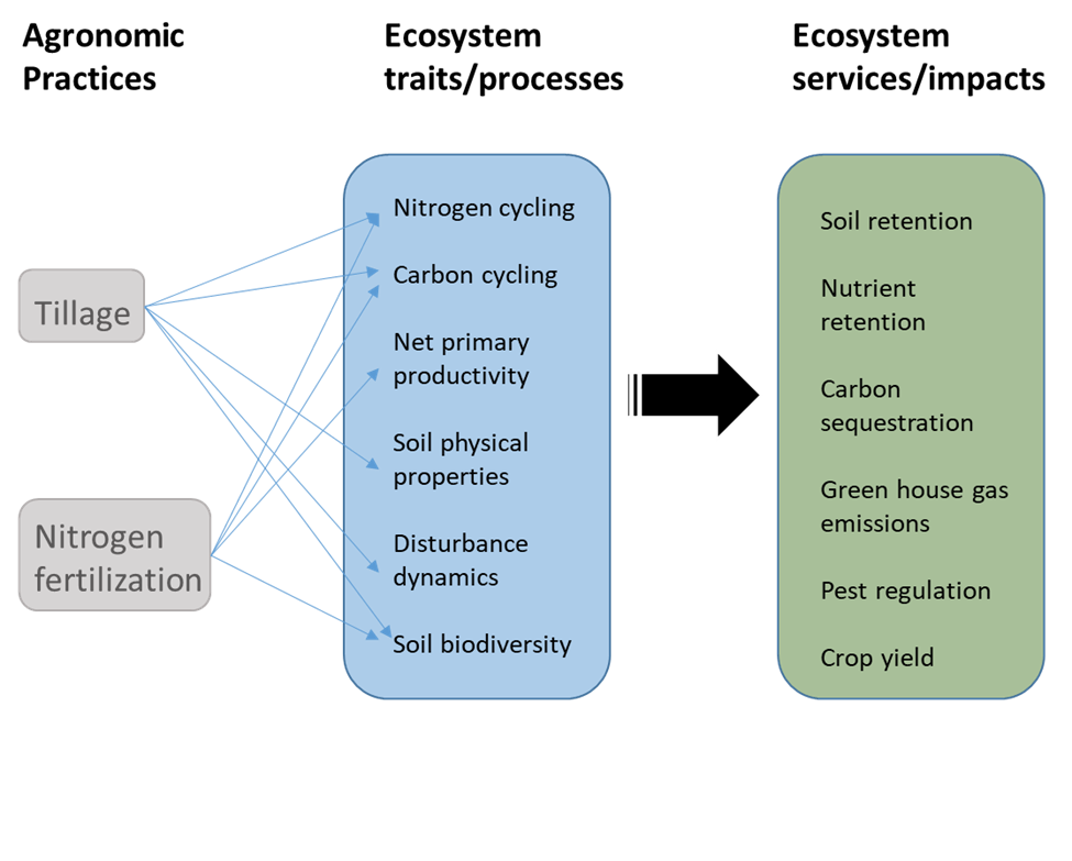
As we develop a better understanding of how agroecosystems function, we are improving our ability to predict how changing farming practices will influence ecosystem processes and how those in turn influence ecosystem services. Figure 7.4 is a conceptual model that outlines how soil tillage and applying nitrogen fertilizer could affect several ecosystem processes that in turn regulate a number of ecosystem services (note the similarity with the model in Figure 2.10). By itself, this figure isn’t very useful. What we need are explicit quantitative models that describe the relationships depicted by each of the arrows. How exactly does increasing tillage frequency alter soil carbon cycling, and how does that in turn affect greenhouse gas emissions?
As you might expect, that is not a particularly easy thing to do, but we have been making considerable progress. The processes that regulate nutrient dynamics in agroecosystems are an example. Much of the nutrients that we apply as fertilizer to farms annoyingly don’t end up in the crop that we intended it for. Instead, various processes channel significant amounts into air and water that travel off the farm and into other ecosystems (see Fig. 3.11). We have developed a better understanding of what ecological processes drive farm nutrient flows and how changes in physical and biological conditions alter their magnitude and what pathway they take. We have used our better understanding to develop mathematical models of the processes (ecological process models) that can predict how changing conditions—such as increasing the amount of fertilizer that is applied—will alter the flows.
Process models are handy for describing the ecological characteristics of individual farms in a way that accounts for their unique conditions and the idiosyncratic ways that farmers manage them. They can also be used as decision support tools to help farmers assess how changing practices will likely alter the ecosystem services that their farms generate. One example is the Nutrient Tracking Tool developed by the US Department of Agriculture. The tool is based on a nutrient process model that describes how nitrogen and phosphorous move through agroecosystems, primarily through the pathways that involve water such as surface runoff and groundwater. Users enter basic environmental characteristics for a target area of interest: things such as soil type, climate, and topography. They also enter specifics about farming practices such as the type of crops, the frequency of tillage, and the amount and timing of fertilizer applications. The model uses that information to estimate how much nitrogen, phosphorous, and sediment leave the target area through water pathways. The model also estimates crop yield and compares results under different management scenarios. Table 7.1 shows some example results for a silage corn (used for animal fodder) field in western Oregon. The baseline management involves practices that are typical for conventionally grown corn in the region. The results under the baseline are compared to those under two management alternatives: (1) growing corn under a no-till system and (2) installing a 15-m grass filter strip along the field margin designed to trap nutrients and sediment. The results indicate that both approaches could significantly reduce nutrient pollution and erosion from the field with minimal or no reduction in crop yield.
| Nutrient and Sediment Export Alteration Estimations Based on Management Systems | |||||
|---|---|---|---|---|---|
| Materials | Baseline Management | No Till | Filter strip | ||
| Nutrients, Sediment, and Crops | Loss or yield | Loss or yield | Change from baseline (%) | Loss or yield | Change from baseline (%) |
| Total Nitrogen (lbs/ac/) | 19.31 | 17.61 | -8.8 | 8.12 | -57.9 |
| Total Phosphorous (lbs/ac/) | 4.48 | 4.08 | -8.9 | 3.29 | -26.6 |
| Sediment (t/ac/) | 0.91 | 0.71 | -22 | 0.26 | -28.5 |
| Crop yield (t/ac) | 15.39 | 15.38 | -0.01 | 15.39 | 0 |
Life Cycle Assessment
Assessing how much ecological impact is generated by a particular farm or a particular set of farming practices is a practical way of describing agroecosystems. We can use that information to assess the degree to which agriculture is helping to push us past the planetary boundaries described in Chapter 1. We can also use impact assessments to help design farming systems that better balance their ecological costs against their social benefits (see Fig. 1.17). A common form of impact assessment is called life cycle assessment (LCA). The name stems from the idea of trying to evaluate the environmental impact of a product or service over its entire life cycle, from creation to demise. For example, we could use LCA methodology to evaluate how much greenhouse gasses are released from the creation, use, and disposal of a pair of cotton pants. That evaluation could include the greenhouse gasses released to grow the cotton, to convert the cotton into textiles, to weave the textiles into pants, to ship the pants to a consumer (or potentially several over the course of its use), and to finally dispose of the tatty remnants in a landfill. But we can also use the LCA approach to evaluate more prescribed chunks of the life cycle—such as just growing the cotton part. Deciding on the life cycle boundary for the analysis is one of the first steps in doing an LCA. We also have to decide on an ecological metric to evaluate. This is typically framed as a measure of some negative impact such as greenhouse gas emissions. The next step in the LCA methodology is to identify all the stages or aspects of production (within the defined boundary of the analysis) that influence the metric. This creates an inventory of impact contributors that we can then get estimates for and tally up. Getting the data to do that is usually one of the hardest parts of doing an LCA. The data can come from direct empirical measurements, but they often come from models such as the one used in Nutrient Tracking Tool.
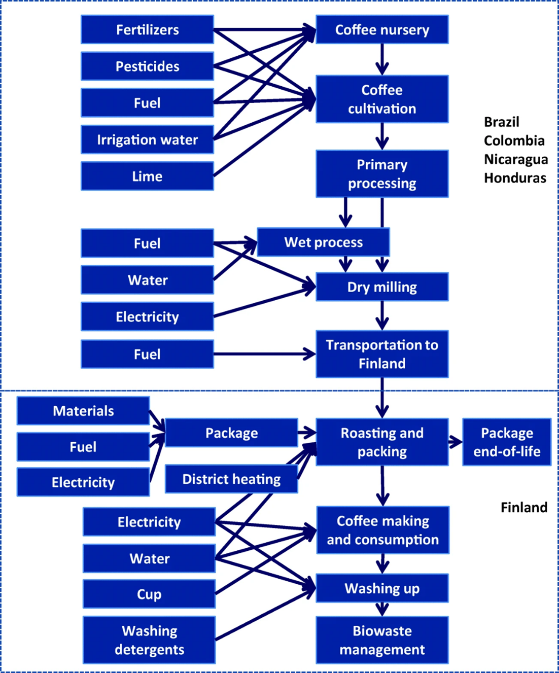
Figure 7.5 is the system boundary for an LCA that estimated the climate impact of drinking a cup of coffee in Finland. The goal of this particular LCA was to identify the points along the journey from coffee field to hip cafe that contributed the most impact. The study boundary included all the greenhouse-gas-generating steps involved in growing the coffee in Latin America, shipping it to Finland, and processing the beans into a cup of coffee. The data for the impact inventory came from a few example farms and a few major coffee purveyors in Finland. Figure 7.6 shows the results. They are organized by the example farms because the vast majority of the climate impact is generated by growing the coffee. The rigmarole of processing and shipping the beans all the way to Finland has comparatively negligible climate impact, although brewing the coffee and dealing with the waste does add a significant chunk. The different climate impact of the farms was mostly caused by differences in the amount of nitrogen fertilizer and lime that was applied. Those differences arose primarily from different local conditions. For instance, the Brazilian farms had exceptionally acidic soils that were mitigated by annual lime applications.
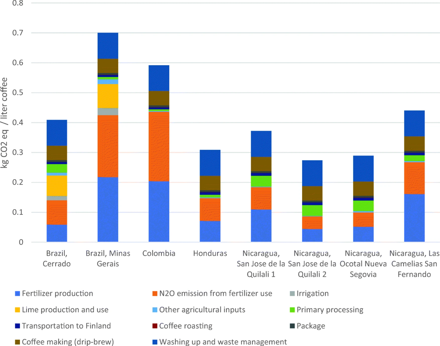
One issue with LCA is that the results are highly sensitive to how we set the boundaries and what metrics we use to assess impact. An important way that coffee affects climate is that it simply isn’t as dense or as old as most tropical forest. Just as with cacao, the significant growth in global coffee production has converted tropical forest into coffee farms. One rough estimate is that global coffee-related deforestation may be as high as 100,000 ha per year.19 The LCA results in Figure 7.6 don’t take this source into account, partly because it was too difficult to evaluate and incorporate the unique land use histories of the individual farms. Also, there is a lot of regional variation in the degree to which coffee production is driving deforestation. Coffee plantations have been expanding at the expense of forest in Honduras but not in Columbia. So, should we add the carbon impact from deforestation to beans grown in Honduras but not Columbia? In addition, the LCA just focused on gross greenhouse gas emissions. But coffee is grown along a shady-to-sunny gradient similar to cacao, and just as with cacao, shady coffee systems sequester considerably more carbon than sunny systems.20 These complications illustrate that the hardest part of doing an LCA is interpreting what the results mean. Because their results are sensitive to seemingly innocuous tweaks in how the analysis is constructed, LCA results are often at the center of bitter debates among people who think that they either downplay or overstate the environmental impact associated with a particular way of farming.
Efficiency Metrics
The outputs of ecological process models and the results of LCA inventories are often framed in efficiency terms. How much climate impact is generated for each cup of coffee that we drink? How many bushels of wheat can we get per acre of land in eastern Washington? How many pollinators do we kill per pesticide application? One reason for their popularity is that efficiency metrics are a handy way of standardizing terms so that we can make comparisons across different agroecosystems—wheat yield in Kansas versus Washington or the climate impact of a kilogram of apples versus a kilogram of oranges. Efficiency metrics are also handy for framing hypotheses about how changes to agroecosystems will alter the benefits we get from them relative to the resources they consume or the damages they create.
All efficiency metrics broadly take the form of a ratio of benefits to costs. When applied to agroecosystems, they are typically framed around three broad costs: land, resources, and environmental impact (Table 7.2).
| Sample Efficiency Metrics For Agroecosystems | ||
|---|---|---|
| Category | General Formulae | Practical Applications |
| Land efficiency | [latex]\frac{\text{biomass production}} {\text{land area } *\text{ time}} \frac{\text{energy fixed}}{\text{land area } *\text{ time}}[/latex] | [latex]\text{Yield}=\frac{\text{ harvested biomass}}{\text{area } *\text{ time}} \text{Net Primary Productivity (NPP)}=\frac{\text{ chemical energy}}{\text{area } *\text{ time}}[/latex] |
| Resource use efficiency | [latex]\frac{\text{physiological process}} {\text{resource consumption}} \frac{\text{output}}{\text{output}}[/latex] | [latex]\text{Water Use Efficiency (WUE}=\frac{\text{photosynthetic rate}}{\text{transpiration rate}} \normalsize \text{Nitrogen Use Efficiency (NUE)}=\frac{\text{Nitrogen in harvest}}{\text{Nitrogen as fertilizer}}[/latex] |
| Environmental impact vs. efficiency | [latex]\frac{\text{environmental impact}}{\text{crop production}} \\ \frac{\text{environmental impact}}{\text{agronomic practice}}[/latex] | [latex]\text{Climate forcing potential}=\frac{\text{CO}_2\text{ equivalent}}{\text{harvested biomass}} \\ \text{Eutrophication potential}=\frac{\text{PO}_4 \text{ equivalent}}{\text{tillage frequency}}[/latex] |
Land Use Efficiency
Perhaps the most common efficiency metric in agriculture is crop yield, or the amount of agricultural production per unit of land (or sea) and period. Yield is analogous to net primary production (NPP). But unlike NPP, yield is usually focused on just the specific fraction of photosynthesis that we harvest such as grain kernels or cotton fiber. Also, yield can be applied at higher trophic levels, such as the amount of milk produced per hectare of pasture per month. That yield metric integrates both how much NPP the pasture generates and how much of that the cows transform into milk.
Yield is a deceptively simple measure that can help us understand both the social benefits and constraints of farming as well the potential ecological impact it generates. On the social side, food and income security are often correlated with the yields that farmers can attain.21 Yield also relates to one of the most fundamental constraints of farming: space. Space for farming is often the hardest, most expensive, and least flexible thing a farmer can manipulate. Consequently, farmers typically try to maximize their crop output per the fixed amount of land they have access to. Access to the most productive farmland has and continues to be one of the main sources of human conflict. The monopolization of high-yielding farmland has historically been one of the main ways that we exert control over others, and unequal access to prime farmland has generated systemic generational inequities in wealth and social status.22 On the ecological side, the environmental impact of farming has historically been broadly correlated with the amount of land we devote to farming. That is because nearly all forms of farming radically transform ecosystems. Maximizing yield is therefore one approach to minimizing farming’s impact is.23
As described in Chapter 1, one result of agro-industrialization and the green revolution has been a prodigious improvement in the average land use efficiency of agriculture. Despite that, there are still large disparities in land use efficiency among regions and individual farmers. One way to conceptualize these differences is an idea called the yield gap. Yield gap is the difference between actual yield and the potentially attainable yield. Attainable yield can be defined abstractly as the yield under ideal conditions, or more practically as the best yields that farmers have attained in reality. In some regions, nearly all the farmers come close to matching the highest practically attainable yield, but in other regions, most farmers routinely struggle to achieve even half of the attainable yield.24
Yield gaps are partly the result of how the traits of specific crops interact with fundamental constraints of climate and soil. For example, wheat farmers in the Southern Great Plains of the United States get generally lower yields than wheat farmers in the Northern Great Plains and in Eastern Washington. That is partly because the climate of the Southern Great Plains is a risky one for growing winter wheat. Winter wheat gets established in the fall, hangs out during the winter, then completes development in the fall and early summer. But summer comes on quickly and hard in places like the Texas Panhandle; in years when it arrives particularly early or hard, it disrupts wheat flower and embryo development, reducing yield.25
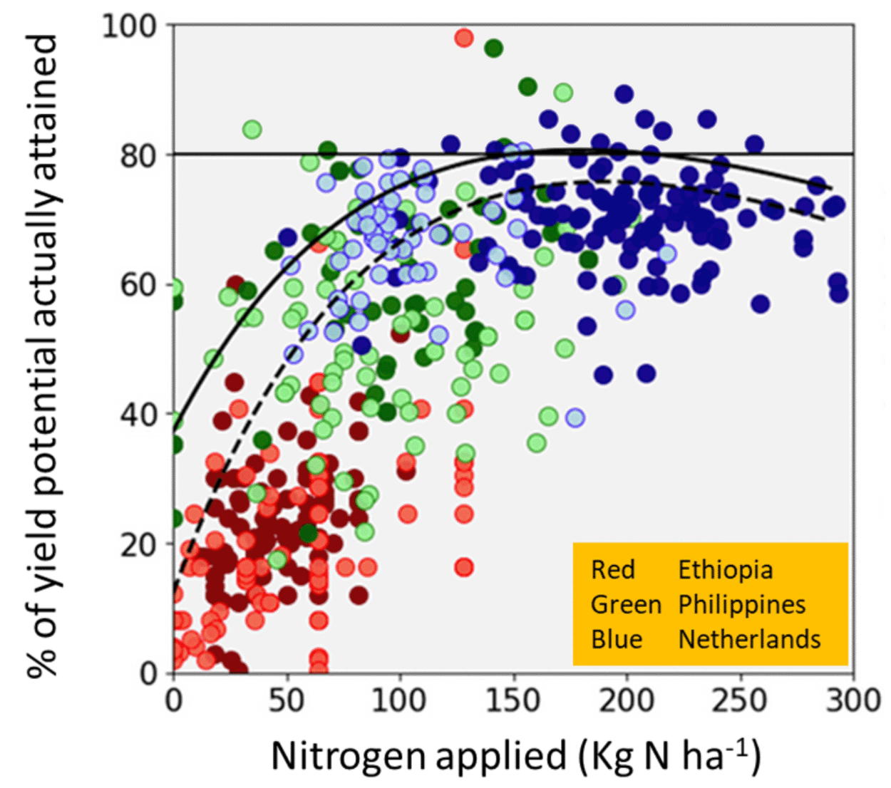
Another important cause of yield gaps is disparity in farmer access to resources. One aspect of this is the disparate ability that farmers have to provide crop resources such as water and nutrients, and in their ability to manage pests. The disparities stem from a complex interaction of economic, social, political, and environmental factors—but poverty is a convenient shorthand explanation. Poor farmers have less ability to ameliorate the limiting conditions for plant growth than better-off farmers. Figure 7.7 is an example of the often strong relationship between the ability to supply crop resources and yield gaps. Relatively poor, smallholder farmers in Ethiopia produce yields that are generally only about 20% of the maximum yields they could theoretically attain. In contrast, relatively rich farmers in the Netherlands routinely get yields that are 80% of their theoretically attainable yield. A significant reason for the difference is that Ethiopian farmers have much less access to and financial ability to apply nitrogen fertilizer than Dutch farmers.26 Farmer resources involve more than just inputs. Farmers benefit from locally relevant agricultural research and crop varieties developed to meet their local needs and constraints. They also benefit from technologies for efficient harvest and transportation; access to markets, credit, and insurance; and knowledge networks for sharing information. Regional and farmer disparities in these types of capacity building resources are another significant cause of yield gaps.
Resource Use Efficiency
Farming uses a lot of resources such as nutrients, water, and energy. These resources cost money and in many cases are of limited supply to farmers. As a result, farmers have a lot of interest in using resources efficiently. In addition, resource use is one of the pathways through which agriculture alters the Earth System. Improving resource use efficiency is therefore an important approach to mitigating agriculture’s environmental impact.
Resource use efficiency metrics come in a bewildering variety of forms. On reason is simply that there are a wide range of different resources. But the different forms also describe different aspects of the system, ask different questions, and are framed from different perspectives. The different ways of describing nitrogen use efficiency (NUE) are an illustration.27 One way to think about NUE is as the nitrogen taken up by a plant relative to the plant available soil nitrogen. This form of NUE is often called nitrogen uptake efficiency (NUpE); it describes the ability of plants to capture available soil nitrogen. Another way to think about NUE is as the yield produced per unit of nitrogen acquired by the plant. This form of NUE is often called nitrogen utilization efficiency (NUtE); it describes the ability of plants to convert the nitrogen they do capture into the specific portion of biomass that we harvest. Probably the most common way of describing NUE is as the ratio of nitrogen in harvested biomass to the nitrogen supplied by farmers. This form of NUE integrates both uptake efficiency and utilization efficiency. Unhelpfully, folks often aren’t explicit about what form of NUE (or other resource efficiency metrics) they are using. There also can be subtler differences in how the numerators or denominators are defined. For instance, the numerator used for nitrogen uptake efficiency could be the total nitrogen available in the soil or just the nitrogen supplied in fertilizer. Be alert to these details.
As with yield, there is considerable variation in resource use efficiency among farming systems, regions, and individual farms. Figure 7.8 is a map of agricultural NUE by country for the year 2014. In this case, NUE is defined as the ratio of nitrogen in harvested biomass relative to the total input of nitrogen to the soil from synthetic fertilizer, manure, nitrogen fixation, and natural deposition. In some countries, NUE is near 100% (i.e., input/output = 1), while in others it’s less than 20%. Much of the variation is related to the financial and capacity disparities that contribute to yield gaps, but the relationships are nuanced. Many poor farmers have high NUE, but that doesn’t necessarily indicate that they have inherently more efficient nutrient management. It mostly reflects the fact that they are severely limited in the amount of nitrogen that they can supply. The small amount of nitrogen input creates a small denominator relative to the large numerator of the nitrogen export via nitrogen hungry crops. In many of these cases, the amount of nitrogen leaving in the harvested crop is greater than the amount that farmers can return to the soil, resulting in gradually diminishing soil fertility in what is known as soil mining.
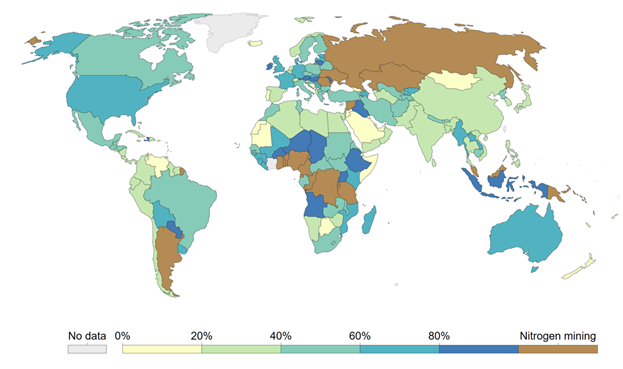
In contrast, richer farmers have a much greater ability to meet the nitrogen needs of their crops. In fact, these farmers often add far more nitrogen to the soil than leaves in harvested biomass so that they generally have lower NUE than poor farmers. Most of the excess nitrogen doesn’t accumulate in the soil but rather leaks away to other ecosystems via water and air. That mismatch between nitrogen inputs and outputs reflects the fact that our ability to supply nitrogen to crops is far greater than the ability of our agroecosystems to capture and utilize the nitrogen. Overall, our agroecosystems are woefully inefficient at capturing and converting supplied nitrogen into crop yield. Globally, only about half of the nitrogen that we supply to fields is converted into harvested crops.28 I describe the main reasons for this inefficiency in Section 7.2.
The various efficiencies of agroecosystems often interact in complex ways. The relationship between yield and nitrogen use efficiency is a great example. We can view the yield gaps in Figure 7.7 through the lens of nitrogen use efficiency. The meager nitrogen supply that many Ethiopian farmers can provide makes them very nitrogen use efficient, but very land use inefficient because of their substantially suboptimal yields. Farmers can increase yield by supplying more nitrogen, but the yield increases eventually plateau. For the farms depicted in Figure 7.7, that plateau in yield return per unit of additional nitrogen is reached at a nitrogen application rate of about 100 kg per hectare; adding any more nitrogen doesn’t consistently result in greater yield. Yet many farmers in the Netherlands routinely apply nitrogen far in excess of 100 kg per hectare. Those extreme nitrogen use farmers are land use efficient but nitrogen use inefficient compared with more moderate nitrogen use farmers.
Environmental Impact Efficiency
A third broad way of describing the efficiency of agroecosystems is in terms of the environmental impact they generate relative to the benefits they produce. One way to frame the impact side of the ratio is in terms of land and resource use, since devoting land and resources to agriculture causes significant Earth System change. We can also use metrics that more explicitly link agricultural activities to specific Earth System changes. These commonly describe the degree to which environmental pollutants such as greenhouse gasses, nutrients, and toxic chemicals cause a measurable change to the Earth System. For example, we can describe the global warming potential associated with the different greenhouse gas emissions from farming activities in terms of their global warming potential, expressed as CO2 equivalent (CO2e) (see Section 4.2 and Figure 4.12). Similarly, we can describe the eutrophication potential of nutrients such as nitrogen and phosphorous, expressed as phosphate equivalents (PO4e). The benefit side of the ratio is typically framed in terms of agricultural outputs in units of biomass or energy. But it is also sometimes framed indirectly in terms of the degree of a useful farming activity, such as the frequency of tillage or the amount of fertilizer applied.
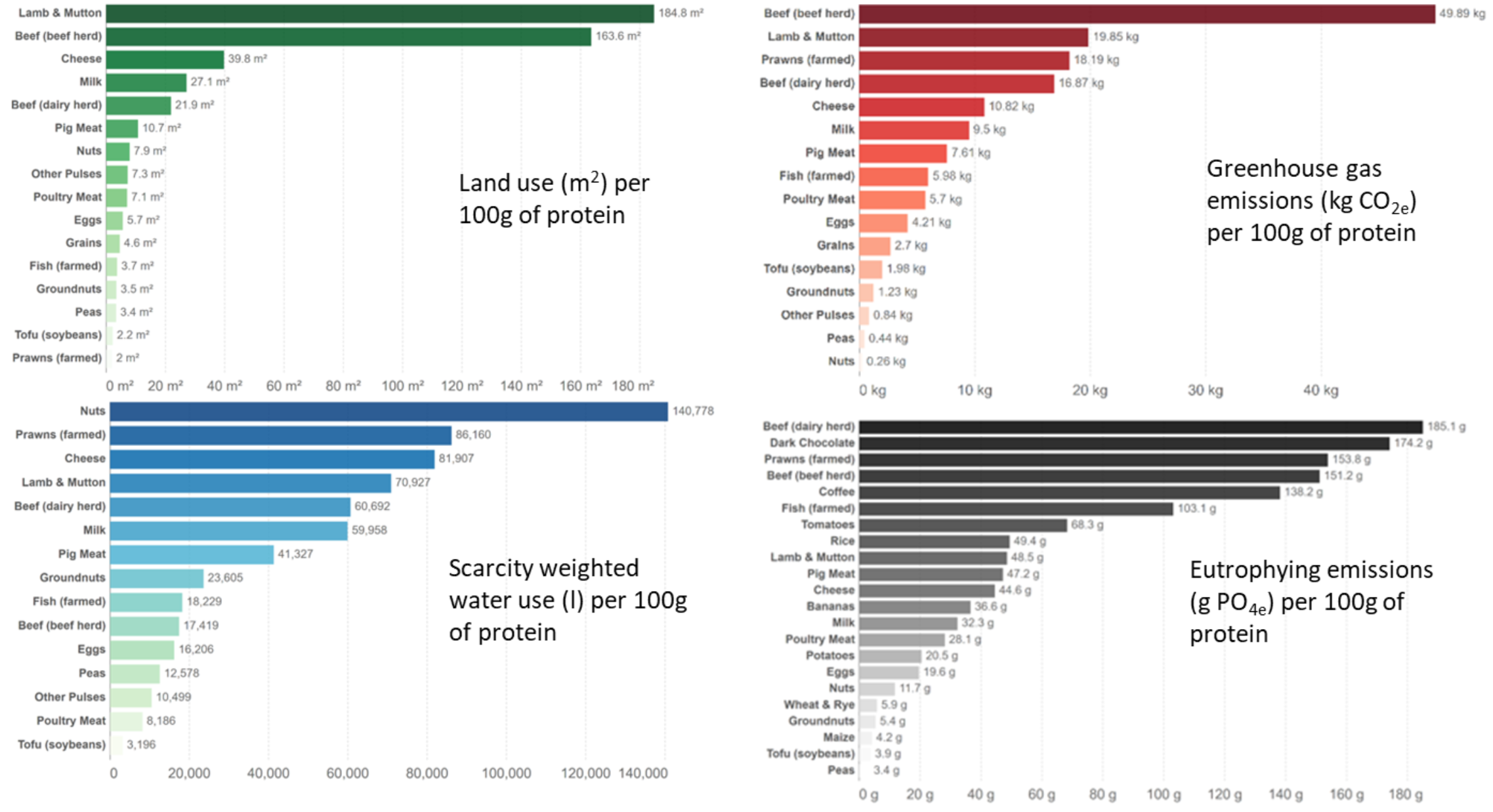
Environmental efficiencies are often called environmental footprints, as in freshwater footprint or carbon footprint. Different crops, regions, and system designs vary greatly in their environmental footprints. Figure 7.9 describes the environmental footprint for a range of foods in terms of the land and water used as well as the global warming and eutrophication potential generated by their production. In this case, the benefit is expressed as a unit of 100 g of protein for each food, which is a more direct measure of the nutritional output than simply biomass or energy. There are many causes for the variation in environmental efficiency among the different foods. But you can probably see one clear pattern: animal-derived foods have relatively higher environmental impact than plant-derived foods. That is related to the inherently inefficient transfer of energy up through trophic levels. I explore this in more detail in Section 7.4.
7.2 The Ecological Impact of Farming
Section 7.2: The Ecological Impact of Farming
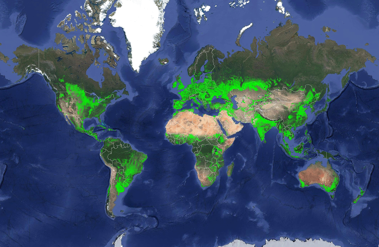
It is difficult to overstate the influence that farming has on the Earth System. Part of the impact stems from sheer scale. About 48% of Earth’s ice-free land is used for agriculture, one-quarter of which is used to grow domesticated crops, and the remaining three-quarters are pastures intensively used for grazing livestock. Roughly another 22% is used for plantation forests.29 Those numbers don’t include the parts of the terrestrial and marine world that we devote to aquaculture. Just the cropland alone covers 1.87 billion ha (Fig. 7.10). But another reason for the outsized impact of agriculture is that so many of our activities are directly or indirectly related to agriculture in one way or another. Excepting our harvest of wild organisms, agriculture is an important underlying motivation for the forces changing biodiversity patterns described in Chapter 6: climate change, domestication, human-assisted species movement, and pollution.
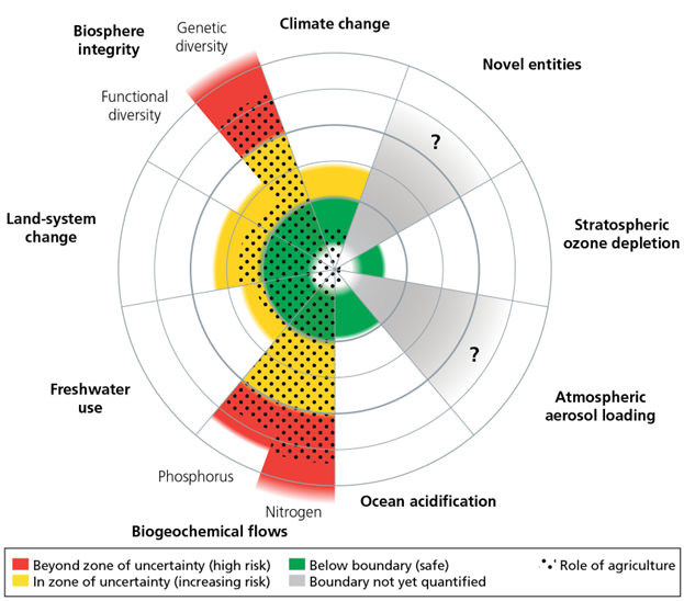
We can also frame agriculture’s impact in terms of the planetary boundary concept that I present in Chapter 1. Figure 7.11 presents an assessment of the contribution that agriculture makes in pushing us past the planetary boundaries set for several Earth System metrics. Agriculture is a primary or significant force driving land system change, nutrient pollution, freshwater use, biodiversity loss, climate change, and ocean acidification.
Let’s look at the ecological impacts in a little more detail.
Climate and Landscape Change
Our agricultural production systems contribute to climate change by increasing the flux of greenhouse gasses to the atmosphere and reducing the flux of greenhouse gasses from the atmosphere into mainly terrestrial reservoirs such as soil and standing vegetation. That happens in two main ways. First, we convert carbon-dense landscapes such as forests and wetlands into agricultural landscapes, which are less carbon dense. Second, many of the day-to-day activities involved in growing crops, processing the harvest into food, and delivering the food to consumers generate greenhouse gasses.
Transforming landscapes for agriculture has historically been the primary way that growing food contributed to climate change. The transformations typically cause a large initial burp of greenhouse gasses to the atmosphere as the carbon stored in cool or waterlogged soil and old tree biomass is abruptly released. The rapid conversion of landscapes into agriculture and other domesticated systems accounted for about a third of our total CO2 emissions from 1750 to 2011. About 133 petagrams (Pg) of C has been released just from the global soil store.30 Perhaps a more visceral statistic is that since the onset of agriculture about 12,000 years ago, we have reduced the total abundance of trees on Earth by about half.31 Over the longer term, agricultural landscapes also tend to sequester far less carbon on an annual basis than forests, grasslands, and wetlands. In Section 3.4, I described the example of the drained wetland soil of the Sacramento–San Joaquin River Delta in California. Farms in the delta release to the atmosphere as much as 341 g C m−2 yr−1 from their soil, while restored wetlands sequester up to up to 397 g C m−2 yr−1 from the atmosphere into the soil.32 Wetland conversions are extreme examples of the general tendency for agricultural landscapes to have abiotic conditions that favor greenhouse-gas-generating processes such as decomposition over processes that sequester carbon. Overall, our creation of agricultural landscapes has reduced the ability of terrestrial ecosystems to act as a sink for atmospheric carbon by slightly more than half.33
Annual greenhouse gas emissions from land use change have been holding roughly steady since 1959.34 That reflects the fact that in some regions, deforestation has slowed and in others agricultural landscapes are being converted back into habitats such as forest and wetlands. But that just means that the net effect on greenhouse gas emissions has stabilized, not that land use change has stopped. Deforestation continues across the increasingly rare landscapes that we haven’t domesticated yet. For instance, the Amazon River basin contains the largest remaining swath of tropical rainforest on the planet, but ongoing land use changes—primarily related to agriculture—have likely already caused the region to switch from being a net sink of greenhouse gasses to being a net exporter.35
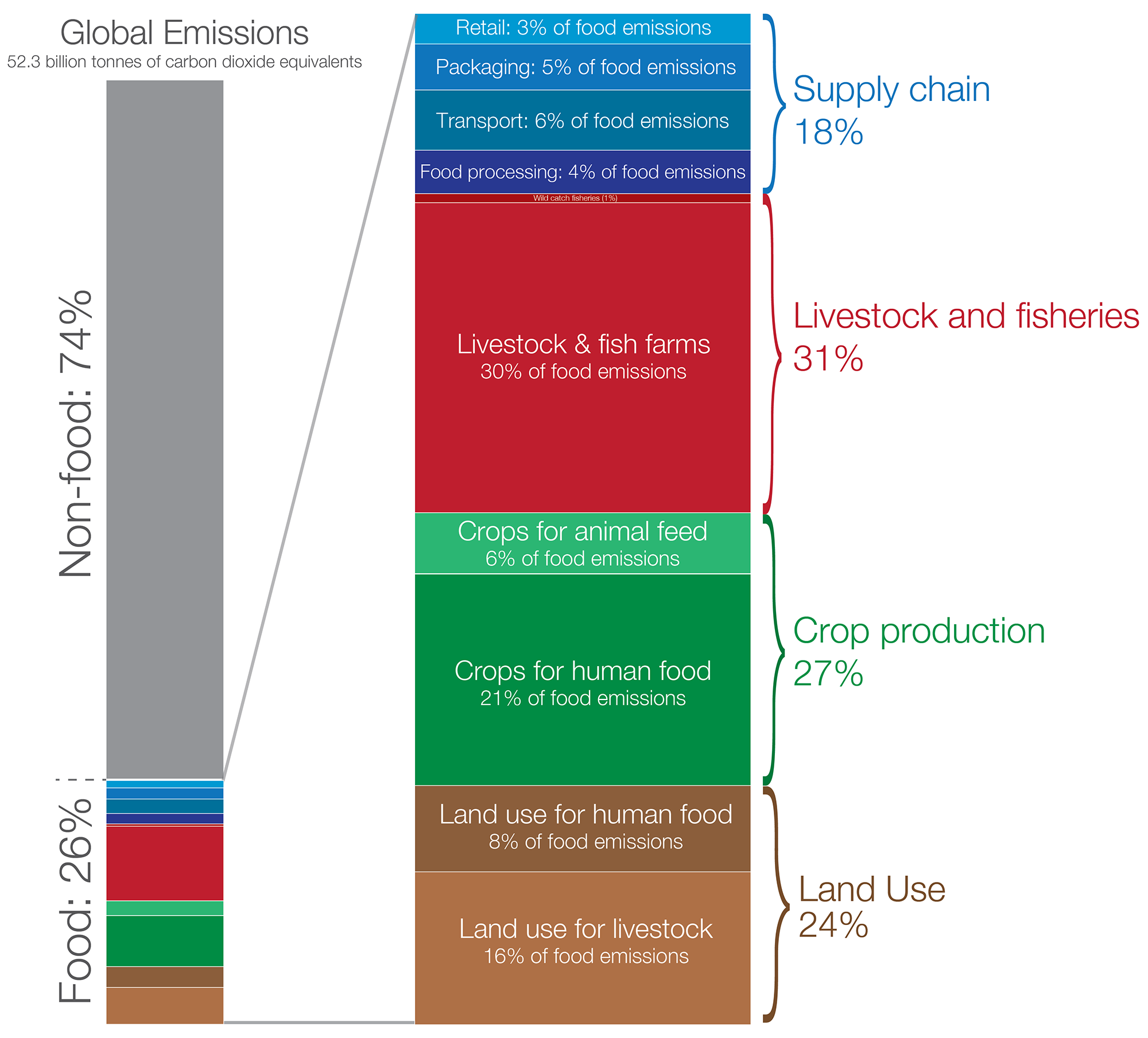
Currently, the greenhouse gas emissions associated with agriculture are roughly equally split between those that are generated as a result of land conversion and those that are generated from the ongoing management of farms and the overall food production system. Food production generates greenhouse gasses in several ways (Figure 7.12), listed below in roughly descending order of their relative climate forcing.
Enteric Fermentation and Manure Management
The guts of ruminant animals such as cows are habitat for microorganisms that generate methane through enteric fermentation (see equation (4.10)). Ruminants as well as other domesticated animals like pigs and chickens also generate a lot of manure, the management of which generates greenhouse gases. Partly because we raise a lot of animals for food and partly because methane is such a potent greenhouse gas, livestock generate roughly a half of all the greenhouse gas emissions (in CO2 equivalents) generated by farming.36
Methane from Waterlogged Agricultural Soils
Microorganisms that thrive in warm, waterlogged soils also generate methane (see equation (4.9)). Probably the most widespread waterlogged agricultural landscapes are periodically flooded rice paddies. Flooded rice systems account for about 16% of farming’s greenhouse gas emissions.37 Another important waterlogged source is freshwater aquaculture. A lot of freshwater aquaculture is done using various forms of constructed wetlands whose soils generate methane. The fish in these wetlands indirectly generate about the same amount of methane per unit of live weight as does a dairy cow directly.38
Nitrogen Fertilizer
Another powerful greenhouse gas released from soil is nitrous oxide (N2O). N2O is a by-product of the coupled nitrification and denitrification reactions of the nitrogen cycle. Some soil bacteria convert ammonium (NH4+) into nitrate (NO3-) (nitrification), while other bacteria convert NO3-</sup first into N2O and finally into nitrogen gas (N2) (denitrification). Depending on conditions, a considerable amount of the N2O can escape to the atmosphere before it is converted to the much more climatically inert N2. These reactions are present in nearly all soils to some degree, but we greatly augment their flow volume (and thus the flow of N2O to the atmosphere) by adding prodigious amounts of nitrogen as both chemical fertilizer and manure. Soil fertilization accounts for about 13% of farming greenhouse gas emissions.39
Fire and Tillage
Burning is one of our oldest agricultural tools. It is particularly good at clearing away weeds and other pests and adding a jolt of nutrients back into the soil. It also converts carbon locked in biomass into greenhouse gasses. Burning is not as commonly used as it once was, but it is still used in some cropping systems and in some regions (see Fig. 1.9). A far more ubiquitous practice is tillage. Soil tillage creates warm, aerated conditions that favor the decomposition of soil organic matter. A significant chunk of the carbon released to the atmosphere through burning and tillage is reabsorbed by the next round of crops, and that tends to mute their net climate impact relative to other farming activities. Still, they act like thumbs on the scale that help to tip agricultural landscapes toward being net greenhouse gas emitters instead of net absorbers.
Food System Energy Use
Fossil-fuel-powered farm machinery—from tractors to irrigation pumps—generate greenhouse gasses. But surprisingly, that on-farm power consumption is responsible for only about 2% of the greenhouse gasses caused by farming. We also generate greenhouse gasses along two other important pathways that extend beyond the farm. One is the mining, manufacture, and transportation of fertilizer, pesticides, and farm equipment. The other is the often long supply chain that converts crops into food products and delivers those into the hands of consumers.
Biogeochemical Flows
A fundamental part of farming is providing crops with ample supplies of nutrients whose availability might otherwise limit crop growth. Our attempts to do this have profoundly altered the Earth System, although that impact has developed only recently. For much of the history of agriculture, the only practical way we could supply crops with nitrogen and phosphorous was with livestock manure and nitrogen-fixing plants like clover. Only a few lucky farmers had access to other sources like guano or deposits of rock phosphate. As a result, much of the practice of farming focused on devising ways to better retain and recycle nitrogen and phosphorous within the agricultural system. These included strategies such as integrating livestock into cropping cycles, developing complicated crop rotations that included nitrogen-fixing species, co-planting species with complementary nutrient use patterns, deploying soil conservation practices that minimized erosion, and when all else failed, simply letting fields lay fallow for stretches of time.
But our focus on nutrient thrift and conservation waned when plant nutrients became much easier to come by. The seismic shift happened with the development of the Haber–Bosch process, which enabled the production of inexpensive and seemingly unlimited amounts of nitrogen fertilizer (see Fig. 1.11). The broader changes associated with the Great Acceleration in the 1950s made that abundant fertilizer increasingly accessible to a wide range of farmers, and as a general rule, those farmers didn’t hesitate to use it. About 86% of the nitrogen and about 96% of the phosphorous we add to the global system is now a result of agriculture, principally from the use of nitrogen and phosphorous fertilizer.4041
The impact of all that fertilizer on the Earth System might not be so bad if most of it stayed in our agroecosystems or got recycled back into them. Unfortunately, nutrient uptake and recycling are no longer strong points of the global food production system. Globally, on average, only about half of the nitrogen and phosphorous that we apply to fields is taken up by crops.4243
Almost all of the applied nitrogen that isn’t taken up by crops or other plants quickly flows away from farms via soil erosion, leaching and runoff, and gaseous emission (the denitrification pathway discussed above). Much of the unused phosphorous also eventually leaves farms primarily via soil erosion, but it often takes a convoluted and slow journey through the soil ecosystem before it does. All the nitrogen and phosphorous flowing away from farms can drive dramatic changes in downstream ecosystems, with the biggest impacts occurring in aquatic ecosystems. I describe those effects in Section 6.7 (see 6.20).
There are five main reasons why our agroecosystems have generally become so poor at taking up and retaining nutrients.
We Mismatch Nutrient Supply and Plant Uptake
Sometimes we apply nutrients when crops aren’t ready to use them, or we give them too much to handle at one time, or microorganisms transform the nutrients in fertilizer into forms that crops find difficult to deal with. We make these errors partly because we don’t fully appreciate the nuanced nutrient needs of crops or what precisely happens to the nutrients that we apply once they enter the complex soil ecosystem. Phosphorous is a good example. We don’t have a complete understanding of what happens to phosphorous in the soil or how it eventually gets taken up by plants. But we know that a lot of the soil phosphorous is immobilized in forms that are inaccessible to plants in the near term. These include phosphorus locked in organic matter, attached to clay surfaces and oxides, and as part of phosphate minerals. Only inorganic phosphorus dissolved in solution is readily (i.e., immediately) available to plants, and it tends to be in chronically short supply in many soils. As a result, there is a persistent risk that crops won’t get enough phosphorous during the often critically short windows that they need it. In the past, there wasn’t much that we could do to mitigate that risk. But now many farmers can hedge the risk by just providing a lot of phosphorous—usually way more than crops need. From 2002 to 2010, global applications of phosphorus fertilizer increased 3.2% per year, much of which never made it to crops and just added to a growing global pool of phosphorous in agricultural soils and in downstream ecosystems.44
We also make nutrient application errors because of all the other difficult constraints involved in farming. For instance, maize growers in the United States sometimes apply fertilizer in the fall rather than the spring even though fall fertilizer applications (when there are few growing plants around to uptake it) results in much higher losses of nitrogen than spring applications.45 Farmers often do this because spring weather and soil conditions can be challenging, and at the same time there is considerable economic pressure to plant as early as possible. This creates a crush of time and resources during the early spring. Applying fertilizer in the fall eases some of the spring pressure.
Crops Aren’t Good at Capturing Soil Nutrients
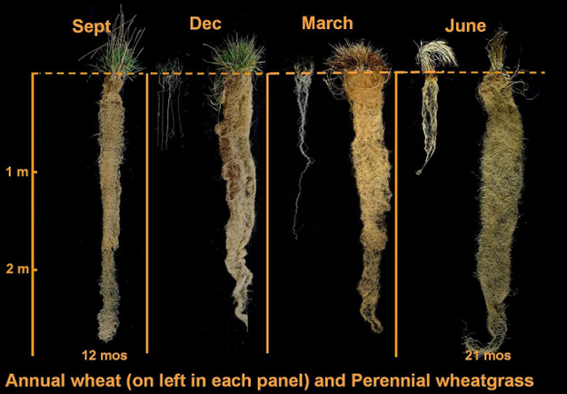
Ideally, we would like to breed crops that are highly efficient at searching for and capturing soil nutrients and then turning those nutrients into precisely the parts of the plant that we harvest for food. We haven’t been able to do this, primarily because it probably isn’t possible for a plant to do both things exceptionally well. To capture nutrients, plants need to allocate resources and effort into things like growing roots or bribing mycorrhizae fungi. That’s energy and resources that aren’t going into the bits we typically harvest, like fruit. Our solution to this conundrum has been to breed crops that are exceptionally good at converting nutrients into harvest (have high allocation efficiency) but that suck at capturing them in the first place (have low uptake efficiency). We then compensate for their low uptake ability by spoon-feeding them lots of nutrients. Our current cultivars of annual wheat are a great illustration of this trade-off (Figure 7.13). I describe these biological trade-offs and our response to them in more detail in Section 7.3.
Agroecosystems Tend to Have Low Biodiversity
There is a generally positive relationship between biodiversity and many ecosystem functions, including nutrient cycling (see Section 2.3). Both the rate at rich soil nutrients are converted into plant available forms and the efficiency at which plants uptake the liberated nutrients increase with biodiversity. We have good evidence of this from a number of experiments done in grassland ecosystems. In one study, researchers created plots in a Minnesota grassland that varied in plant species richness from monocultures up to 16 species. After 23 years, the 16 species plots had 30% to 90% more nitrogen, potassium, calcium, and magnesium in their soil than the monoculture plots. They also had 150% to 370% more of those nutrients captured in living plant biomass than the monoculture plots.46
All three mechanisms underlying the general biodiversity-function relationship described in Chapter 2 play a role in nutrient cycling. First, some plants and soil organisms have unique traits that make them particularly important in terms of nutrient availability or uptake. Nitrogen-fixing plants generate soil nitrogen in forms that are particularly easy for plants to uptake; nitrogen added to fields via nitrogen-fixing cover crops appears to be assimilated by crops with a higher efficiency than nitrogen applied as a chemical fertilizer.47 Second, species often have complementary resource capture. For instance, the annual wheat and perennial wheatgrass in Figure 7.13 access nutrients from different parts of the soil and during different times of the year. In the Minnesota grassland experiment, the 16 species in the high-diversity plots had distinct nutrient uptake niches—legumes were particularly good at generating plant available nitrogen; other forbs were particularly good at capturing potassium, calcium, and magnesium and then releasing them back to the soil; grasses were particularly good at all-purpose nutrient capture. Finally, different species often help facilitate nutrient uptake among each other. The complexity of phosphorous uptake is an example. Soil microorganism and plant roots produce phosphatase enzymes that release organically bound phosphorous into inorganic bioavailable forms. In addition, arbuscular mycorrhizal fungi form symbioses with plant roots, getting carbon from the plant in exchange for delivering phosphorus and other nutrients. Phosphatase activity (i.e., the rate at rich inorganic phosphorous is being mobilized) and the overall efficiency of phosphorous uptake by plants are greater in more biodiverse systems.48 All of those mechanisms tend to foster more complete and efficient nutrient cycling as the biodiversity of the system increases. But agroecosystems tend to have low biodiversity; we manage many as monocultures. That makes retaining and recycling nutrients on farms a difficult task.
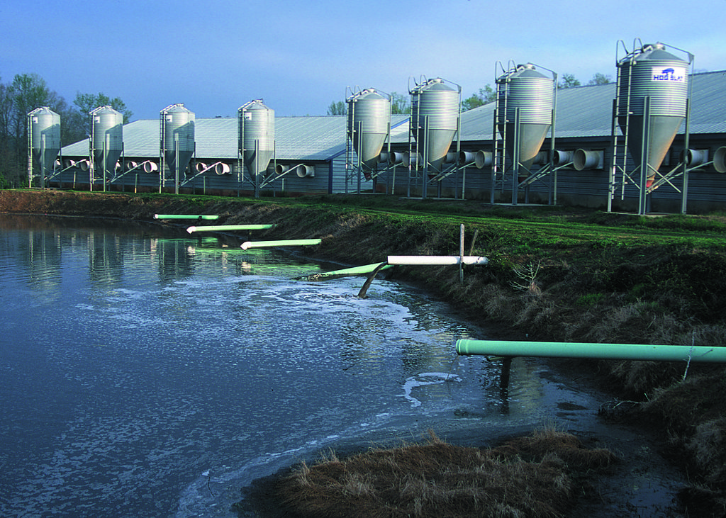
Another aspect of how the reduced biodiversity of agroecosystems hinders nutrient cycling manifests itself at the larger scale of our entire food system. The increased availability of chemical fertilizers and more efficient transportation networks have allowed many farmers to spatially separate growing crops and raising livestock, which by extension separates the nutrients in manure from the soil where they came from. We sometimes try to get the nutrients back to farm soils, albeit usually not the same soil they started out in. But the typical process is riddled with inefficiencies. For instance, manure from concentrated animal feeding operations (CAFOs) is often stored in open anaerobic lagoons (Figure 7.14). These are a significant source of greenhouse gasses (see above) as well as ammonia (NH3). The ponds also leak and are vulnerable to catastrophic failures. Using the manure from CAFOs is often as much about staying on top of the never-ending flow of feces than it is about precisely allocating nutrients that meet crop needs.
A similar problem exists for our own manure, since most of us now live far from where our food was grown. One study estimates that 27% of the nitrogen and 42% of the phosphorus entering the landscape surrounding the US side of the Great Lakes came from livestock manure, with an additional 2% of each coming from suburban septic systems.49 Much of the livestock-derived nutrients are entering the landscape as applied manure fertilizer, so a portion of it does make its way back into crops instead of flowing into the Great Lakes. But the inefficiencies associated with the spatial disarticulation exacerbate the nutrient leakiness of the whole food system.
Fire, Tillage, and Soil Erosion
Field burning and tillage move soil nitrogen to the atmosphere in the form of the greenhouse gas nitrous oxide, as described above. In addition, soil erosion is one of the principal ways that nutrients flow off agricultural fields. Many of the activities associated with farming, such as tillage, harvesting crops, and creating annual-dominated systems, exacerbate soil erosion. On average, soil erosion rates are an order of magnitude higher in agricultural landscapes than other landscape types.50 Given how widespread our agroecosystems are, the scale of the resulting soil loss is prodigious. Overall, the main agricultural landscapes (annual crops, permanent crops, and managed pasture) are responsible for 54% of global soil erosion—that is equal to about 23 Pg of soil per year as of 2015. Annual croplands contributed most of that erosion. Even though annual crops covered only about 16% of land in 2015, they were responsible for an estimated 41% of global soil erosion.51
All that eroding soil carries with it a lot of nutrients, particularly phosphorous. Globally, agricultural soils lose an average of 5.9 kg P ha-1 yr-1 due to soil erosion by water, with a total global loss of 6.3 Tg P yr-1.52 That phosphorus fuels the eutrophication of downstream ecosystems, but it also contributes to an ongoing loss of soil fertility. Figure 7.15 is an estimated global phosphorous budget for agricultural soils. We compensate for the erosional loss of soil phosphorous by adding back an average of 8.8 kg P ha-1 yr-1 in the form of chemical fertilizer. We also add phosphorous in the organic forms of manure and plant biomass. Organic phosphorous also leaves in the form of the harvested crop biomass. In this budget, the crop losses are subtracted from the organic inputs and reported as a net organic input value called “organic P management”—you can think of that as roughly the amount of crop phosphorous that gets returned to the soil.
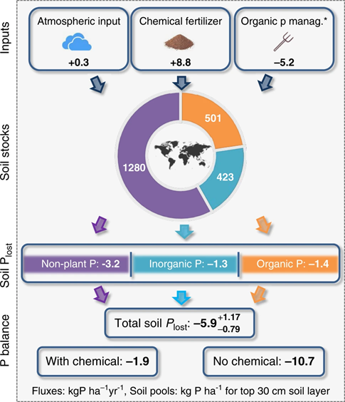
Globally, more phosphorous leaves in the harvest than is added back as organic forms, with an average net loss of 5.2 kg P ha-1 yr-1. All together, even with the massive input of chemical fertilizer, global agricultural soils are experiencing a net annual phosphorous decline of 1.9 kg P ha-1 yr-1. Not only are we degrading the ability of downstream aquatic ecosystems to provide food in the form of fisheries, but we also aren’t even maintaining the ecological capacity of terrestrial agroecosystems to provide food. As with other aspects of farming’s ecological impact, there is considerable variation across regions, farming systems, and individual farms. That variation is driven by environmental differences, differences in soil and nutrient management practices, social differences, and the different economic constraints facing farmers.
Ammonia Volatilization
One of the many biochemical processes mediated by soil microorganisms converts urea (CO(NH2)2) into carbamic acid (H2NCOOH), which quickly dissociates into ammonia (NH3) and carbon dioxide (CO2). Under many conditions, the ammonia gas quickly hydrolyzes into ammonium (NH4+), which can be taken up by plants. Unfortunately, conditions in many agroecosystems often favor the flow of ammonia to the atmosphere instead of into solution in the soil. Perhaps the biggest cause is simply that we apply prodigious amounts of urea in the various formulations of chemical fertilizer as well as manure. We also typically apply the fertilizer to the soil surface, which promotes the escape of ammonia to the atmosphere. A range of other factors such as temperature, moisture, and soil pH also influence the degree of ammonia volatilization. Globally, an average of 10% to 20% of the nitrogen we apply to agroecosystems is lost as ammonia gas, although in many regions and systems, the loss is considerably higher. In total, the agricultural leak of ammonia accounts for about 43% of the global emission of ammonia to the atmosphere.53
Freshwater Use
It takes a lot of fresh water to grow our crops and raise our livestock. At the beginning of the twenty-first century, agricultural production appropriated an average of 8,363 cubic gigameters (Gm3) of water per year, 92% of all the water humanity uses.54 That sounds like—and is—a lot of water, but it is a bit difficult to contextualize how that appropriation affects the Earth System. One of the primary impacts of our water use is to simply make water less available to other users. But the degree to which that happens depends as much on the overall supply of water as it does on how much water we use. The same amount of water use will have a bigger impact on water availability in an arid region than in a wet one. Also, we use water in a few distinct ways, with various effects on water availability. That is why I used the more nebulous-sounding appropriate to describe the 8,363 Gm3. Another commonly used term is the water footprint.
Water scientists have developed a framework to describe the nuances of our water use and to help contextualize the impact it has. The water footprint has three components.
Green Water
The green water footprint is the amount of rainwater that is directly sent right back to the atmosphere via evapotranspiration from human landscapes or that is incorporated into products like crops. Overall, green water makes up 74% of our total global water footprint, and almost all of that is a result of the rainwater evapotranspired from agricultural landscapes or incorporated into the bodies of crops and livestock.55 Although green water is the biggest component of our overall water footprint, in some ways it is the most benign in Earth System terms. Evapotranspiration from agricultural landscapes is roughly comparable (with some notable exceptions) to other vegetated landscape types, so the rainfall that falls on an agricultural field and is consumed by crops doesn’t often reduce water availability for other users in a watershed any more than if the landscape was vegetated with something else like a grassland or forest.
Blue Water
The blue water footprint is the fresh water we withdraw and consume (in various ways) from aquifers, lakes, rivers, and streams. Blue water makes up about 11% of our total water footprint, and agriculture accounts for about 70% of it in the form of water withdrawals to irrigate crops or to provide water for domesticated animals.5657 Although it’s a relatively small proportion of our overall footprint, blue water has a much bigger impact on the Earth System than green water, partly because it is such an attractive source of water. In contrast to rainfall, which can suffer wild and fickle swings in availability, the supply of water flowing through aquifers, rivers, and streams is more even and dependable. We have enhanced that dependability with dams and other water storage devices. The greater dependability of blue water supplies can be particularly important (and attractive) to water users in arid and semiarid climates or in climates that experience big swings in the seasonal timing of rainfall. As a result, we tend to use a lot of blue water when and where overall water availability is low. Our heavy use of blue water during periods of low water availability is one of the main ways that our water use causes water scarcity and negative impacts.
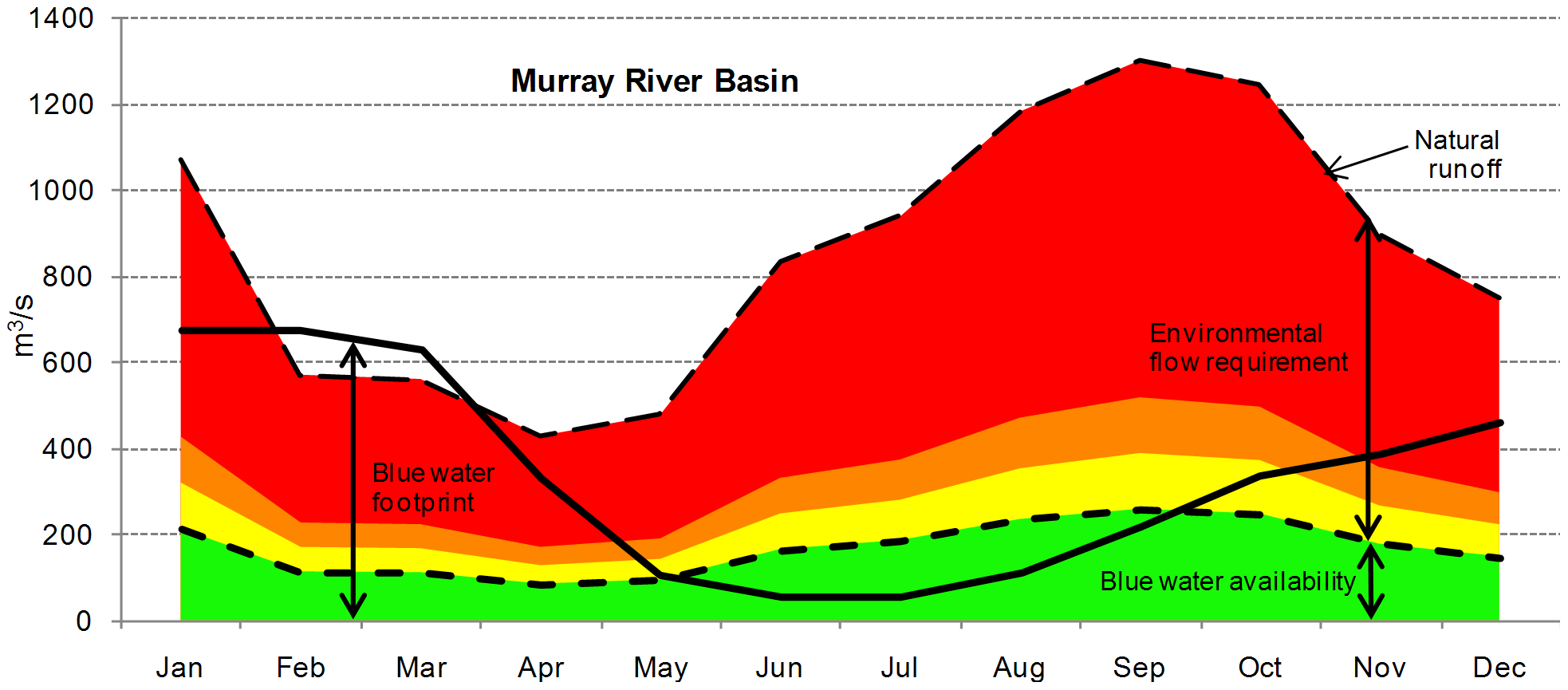
An example comes from the Murray-Darling River basin in southeastern Australia. The Murray-Darling is Australia’s most important agricultural region, similar in many ways to the Central Valley of California. Like in the Central Valley, water availability is highly seasonal—relatively abundant during winter and annoyingly low during the main crop-growing season. Irrigation linked to a complex storage and distribution network keeps crops growing during the dry time. But that consumptive water use makes water less available to other water users, principally aquatic species such as the Murray cod (Maccullochella peelii). Figure 7.16 illustrates how the environmental impact of that blue water use varies seasonally with the ebb and flow of both runoff and the irrigation needs of the region’s crops. It partitions the total runoff (blue water) into the estimated amount needed to support the aquatic ecosystem (the environmental flow requirement) and the remaining water that could be used for other purposes like irrigation (the environmentally safe available blue water). For much of the year, water withdraws (the blue water footprint). exceed the environmentally safe available blue water. The impact is most severe in late summer when most of the environmental flow requirement is diverted to crops. Not surprisingly, the region’s aquatic ecosystem—headlined by the Murray cod—has been severely degraded.58
Gray Water
The gray water footprint is the blue water we make unusable by polluting it; it is estimated as the volume of clean water needed to dilute pollutants down to some ambient water quality standard. Gray water makes up about 15% of our total water footprint, and agriculture is a significant contributor in the form of eroded soil particles, nutrient eutrophication, pesticides, and salts and other minerals accumulated in irrigated soils.5960 Gray water not only reduces the availability of water; the component pollutants can also directly affect organisms and ecosystem functions. Like with blue water, these impacts can be particularly severe during times of low overall water availability.
The blue and gray water footprints of agriculture make water unavailable for other uses and users in a watershed. These include water for industrial purposes, human drinking water, and water to maintain urban landscapes—the other 30% of our blue water footprint. And, of course, it also includes the ecosystems and associated biodiversity that depend on fresh water. These ecosystems in turn provide human communities with a wide range of ecosystem services such as fisheries and recreation.
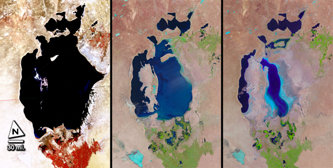
A notorious example of agricultural-driven water scarcity is the recent history of the Aral Sea. Starting in the 1950s, the region experienced a rapid expansion of irrigated agriculture, primarily for cotton. Most off the available blue water that flowed into the sea was eventually diverted to farms—a larger-scale version of the Murray River basin example. With most of its inflow diverted for irrigation, what was once the fourth-largest lake in the world is now a handful of smaller, saltier lakes scattered along the fringes of a desert (Figure 7.17). The transformation has been an environmental disaster.61 First, fisheries collapsed, devastating the local communities that depended on them. Then, as the water disappeared altogether, vast dust storms laden with salt and agricultural chemicals blanketed the region. Even the agriculture that was the proximate cause of the lake’s decline began to suffer. Salt blowing off the dry lakebed contaminated nearby fields, reducing their productivity. Without the moderating influence of the large water body, temperature fluctuations became more extreme, leading to harsher winters and hotter, drier summers that required even more irrigation to sustain crops. Unfortunately, the Aral Sea is not an anomaly. Two-thirds of the people living on Earth (4 billion people) now experience severe water scarcity for at least part of the year.62
Biodiversity
Agriculture changes biodiversity in two overlapping and not particularly distinct phases: (1) the initial conversion of relatively biodiverse ecosystems into generally less biodiverse agroecosystems and (2) the ongoing management of agroecosystems.
Conversion
The creation of agroecosystems radically transforms broad suites of ecosystem traits and processes, usually abruptly. Ecologists call such dramatic ecosystem reorganizations regime shifts. The name is particularly apt for reorganizations into agroecosystems because we directly take control and assert our dominance over our creation—or at least we try to. As described in Chapter 6 (see Section 6.4), the new ecosystems are not only radically different, but they also tend to have less biodiversity than the ecosystems they replaced. The overarching reason for this lack of biodiversity is that we typically design agroecosystems to support a few favored types (i.e., genes, species, functions, habitats) or to generate a narrow suite of ecosystem services. We finely tune environmental conditions to optimally support our favored biodiversity and goals, and we make those optimal conditions as homogenous in space and time as possible. That constrains and homogenizes biodiversity across metrics and scales—from the functional diversity of the soil microbiome, to the species richness of a farm, to the habitat turnover across a region. For instance, global croplands support roughly 40% less local species richness than natural vegetation under minimal human use.63 Such dramatic reductions make landscape conversion into agriculture one of the primary causes of biodiversity loss—responsible for as much as 80% of global biodiversity loss.64
The magnitude of the loss is exacerbated by the fact that much of our ongoing landscape conversion is taking place in the most biodiverse regions of the planet.65 From 1980 to 2000, more than 55% of the land that was converted to agriculture came from the world’s dwindling supply of pristine tropical forest.66 These ongoing land use changes are negatively affecting a broad swath of organisms. One estimate of the magnitude of these effects comes from a study that modeled how the amount of habitat for 19,859 species of terrestrial vertebrates will change if current patterns of agricultural expansion continue. The study projected that nearly all (88%) of the studied species will lose at least some habitat to agricultural expansion by 2050, with a global average habitat loss of 6%. Some species will suffer much more substantial losses; about 6% of the studied species will lose more than 25% of their habitat.67
As described above and in Section 6.4, there is considerable variation in the design of agroecosystems and in the amount and type of biodiversity they support. The range of coffee and cacao farming systems are examples (see Fig. 7.3). Some agroecosystems even support broadly higher biodiversity than non-domesticated landscapes. The cork oak agro-silvo-pasture system of the Mediterranean basin described in Chapter 6 is an example (see Fig. 6.8). Relatively biodiverse agroecosystems typically use multiple domesticated species that have complementary functional traits, employ spatially or temporally diverse management practices, and integrate some more natural landscape types as part of the system. For instance, the cork oak ecosystem includes oak woodlands, pasture for grazing animals, habitat for game animals, and cropland. These elements are managed in different ways, creating a complex patchwork of abiotic conditions, states of succession, and habitats, and in turn fostering a rich assortment of non-domesticated plant and animal species, including threatened species such as the Iberian lynx (Lynx pardinus) that do poorly in other domesticated landscapes.
Relatively diverse forms of agriculture such as agroforestry and agro-silvo-pasture systems used to be more commonly practiced than they are today. They were popular partly because they generated a diversity of food and other useful products locally and on a relatively small amount of land. Also, as mentioned above, integrating livestock with crop production was one of the few ways we had of maintaining soil fertility. But these functionally diverse systems began to decline with the spread of agro-industrialization and the other changes associated with the Great Acceleration (see Chap. 1 and Section 6.4). Chemical fertilizers, mechanization, efficient transportation networks, globalized markets, increased global social connectivity, and the human-assisted spread of non-domesticated organisms changed the basic goals and constraints that influenced how farmers designed their agroecosystems. The changes made possible and incentivized the specialization of farms. Instead of growing multiple types of crops and closely integrating growing crops and raising animals, farms in many places have increasingly become specialists at producing one type of crop: cereal grains or vegetables or cows or sheep or timber or fish. Agro-industrialization also gave many farmers increasing control over the biophysical environment of farms. We used that power to design conditions that precisely suited the few crop species that each farm was specialized for. In turn, we bred crops to optimize the narrow conditions we created for them, reducing crop genetic and functional diversity.
Farmers around the world have increasingly operated under a globalized set of similar constraints and pressures. Before the Great Acceleration, farm designs primarily reflected adaptations to unique local conditions of climate, soil, politics, economics, and culture. Farm designs still reflect local conditions, but they also increasingly reflect more universal constraints and goals. Today, farmers grow crop types that are favored by consumers who may live in disparate places but who have similar diets and tastes—or at least they are far more similar than they were just a generation or two ago. Farmers also want varieties of those crops that ship and store well, can be grown and processed using standardized inputs and machinery, and are resistant to a similar list of pests. One result of the globalization of goals has been the emergence of global agricultural anthromes that are based around a few crop species. These systems use genetically similar (often identical) crop varieties, are managed in ways that create similar abiotic conditions, and support similar suites of ancillary species such as pests. An example is the maize anthrome (Figure 7.18). Just five anthrome types (wheat, rice, maize, barley, and soybeans) constitute 60% of our cropland.68
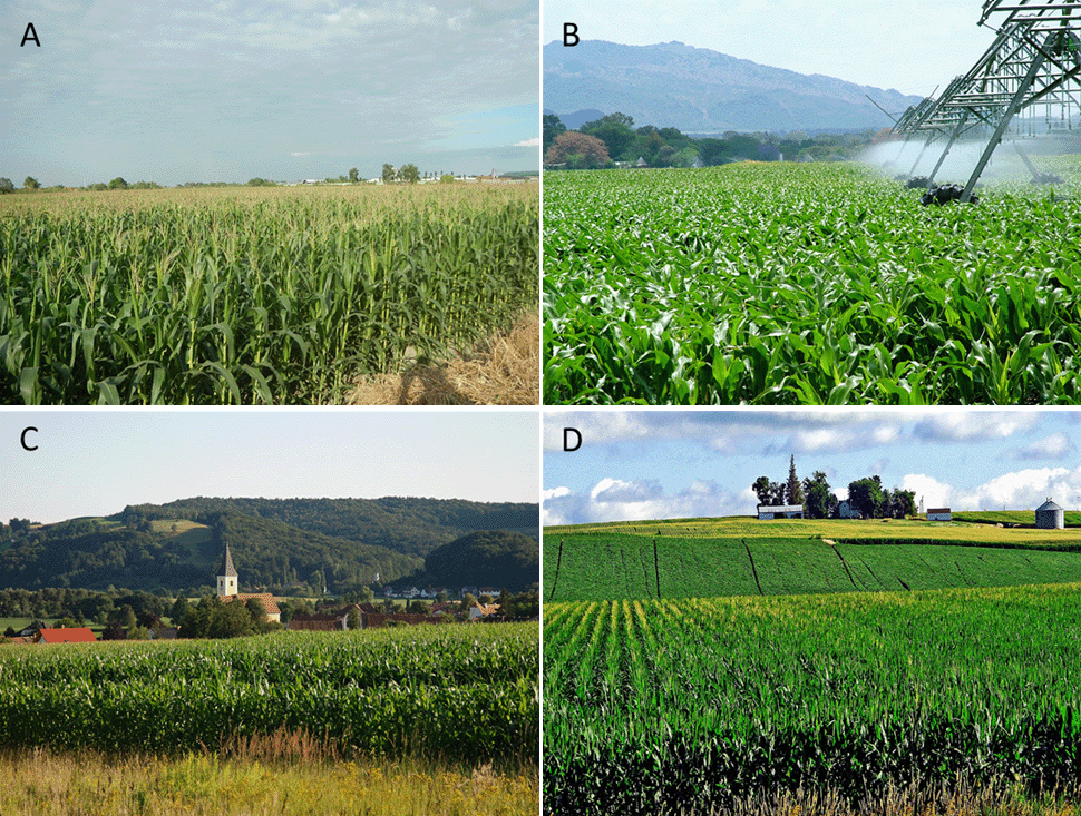
An illustration of how these trends have tended to reduce local-scale biodiversity comes from the farm fields of central Germany. Since the region’s agricultural systems began industrializing in the 1950s, the number of crop species being farmed has decreased from 25 to 16 species (as of 2009). Over the same period, overall plant species richness (including non-domesticated species) decreased by 71% at the scale of individual fields and by 23% at the scale of the entire region.69 The specific plant associations found on individual farms have also become more similar to each other; that is, the spatial turnover in species from farm to farm has decreased. In the 1950s, the types of plants found on individual farms—both the crops and non-crops—were strongly influenced by differences in soil type that affected soil parameters such as soil pH and nitrogen levels. The region’s farmers have been able to smooth out the differences in pH and nitrogen, resulting in a more homogenous set of plant species on each farm.
The landscape homogenization of plant species composition in Germany is an illustration of how the creation of agroecosystems transforms entire landscapes. The same environmental and human social factors that constrain and motivate the design of individual farms also shape the characteristics of agricultural landscapes (Fig. 7.19). In turn, landscape-scale patterns strongly influence the amount and type of biodiversity that agricultural landscapes support. Some agricultural landscapes are composed of just a few crops and management types, while others have a diverse array of different crops or farming systems. Some landscapes are composed almost entirely of domesticated habitats, while others include non-domesticated habitats like wetlands and forest as well as seminatural habitats like hedgerows and grassy field margins. Landscapes also differ in how their habitat types are spatially arranged. For instance, in northwest Germany, fields are small, organized in irregular patterns across the landscape, and are intricately intermixed with natural and seminatural habitat, creating a complex mosaic. But in Minnesota, fields are large and organized in a regular grid that creates a simpler, more homogenous landscape (Fig. 7.19).
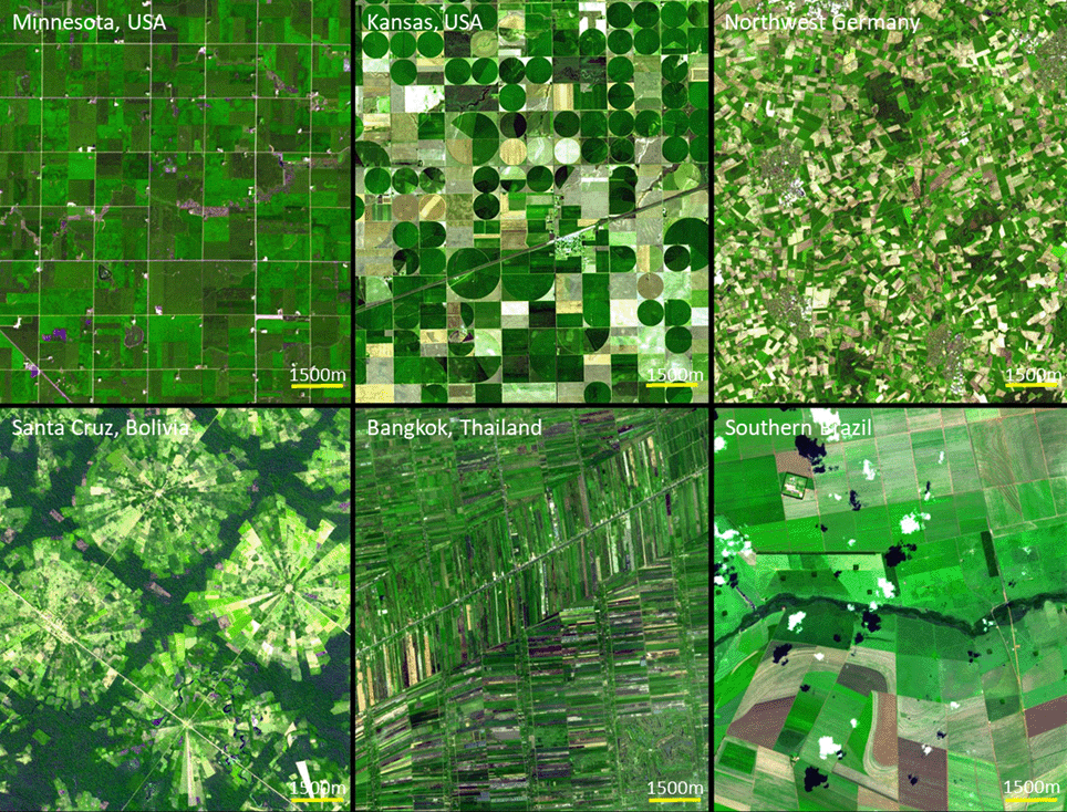
Complex agricultural landscapes that contain diverse habitat types organized in intricate patterns tend to support higher levels of biodiversity than simpler landscapes with a few uniformly distributed habitats.70 That relationship partly arises from the simple fact that a greater variety of habitats supports a greater variety of organisms. In addition, many mobile organisms benefit from the more complex spatial arrangement of habitat. Hedgerows provide an example. Farmers in many parts of the world have long used woody perennial hedges to delineate property lines, as windbreaks, and to slow soil erosion (Fig. 7.20). Partly because they are long and thin, hedgerows pack a lot of habitat complexity into a small area. The central core can be as dark and quiet as an old-growth forest, while the edge can be as bright and airy as a savannah. That environmental diversity supports a diversity of organisms. In Belgium, hedgerows support both grassland and forest plant species so that in aggregate they contain more overall species of plants than nearby forest areas.71 The high plant diversity in turn supports a diversity of animals. These include animals that call hedgerows home as well as ones that visit hedgerows for resources such as flowers and other food. In the Central Valley of California, for instance, birds are three to six times more abundant and two to three times more species rich along hedgerows than along bare or weedy field margins.72 Hedgerows also provide safe passageways that link larger patches of natural and semi-natural habitat, which can allow populations of species that depend on natural habitat to persist in agricultural landscapes even through their required habitat is fragmented and scattered across expanses of inhospitable farmland.73
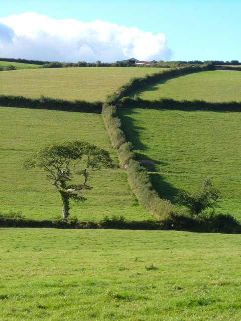
The same forces that have tended to homogenize farm designs have also tended to reduce the complexity of agricultural landscapes. The homogenization comes both from the loss of nonfarm habitats in the landscape such as wetlands, bits of forest, and unmanaged margins like hedgerows as well as from declining diversity of the crops themselves.74 The trend is particularly noticeable in the United States. In 1940, 88% of US counties grew more than 10 major crops, but only 2% of counties did so in 2017. Since 2000, the spatial distributions of most crops have become highly concentrated in a few regions that specialize on growing them.75 There is evidence that the ongoing homogenization of regional agricultural landscapes is contributing to broader biodiversity loss. One large study conducted across Europe and North America found that the loss of semi-natural habitat, increasing field size, and decreasing crop richness were all associated with reduced biodiversity—measured using an index that included plants, bees, butterflies, hoverflies, carabid beetles, spiders, and birds.76 One specific example comes from the US Midwest, where local crop richness is currently half of what it was in the 1900s. The species richness of the region’s bumblebees has also declined by 20%. Intriguingly, the timing of the landscape changes and the bumblebee declines are in sync: both happened primarily after the 1940s. Even though the region was dominated by agriculture in the 1940s, it still had a rich assortment of bumblebees. That seems to be at least partly because the diverse cropping systems as well as more abundant bits of non-crop habitat provided a diverse range of floral resources for bumble bees. Those resources also varied across space and seasonally. But as the landscape became more habitat homogenized over the next 80 years, so did the floral resources, which in turn contributed to the loss of bumblebee richness.77
Another compelling example of how our design of agricultural landscapes influences biodiversity comes from an unplanned experiment stemming from the Cold War. During the Cold War, many countries in Eastern Europe forcibly collectivized private farms. Individual farm fields were merged into larger ones, and their hedgerow boundary markers were removed. In Western Europe, farms remained private, and government policies helped to maintain their small size and complex arrangement even in the face of agro-industrialization. The landscape differences can still be seen today. Farms in the former East Germany are an average six times larger than farms in the former West Germany, while fields in the west have more than 70% longer edges than those in the east.78 The difference in field size and shape does not affect the local species richness of fields; individual fields in the east and west have the same average species richness of birds and insects. Instead, levels of local species richness are strongly influenced by how fields are managed on a day-to-day basis. Organically managed farms in both the east and west have greater bird and insect species richness than conventionally managed farms. But field shape and size do affect biodiversity at the landscape scale. In aggregate, the more complex agricultural landscape in the west supports considerably more species of birds and insects than the simpler landscape in the east, and the effect is even greater than that caused by the day-to-day management of individual fields. Landscapes dominated by small-scale but conventionally managed fields have greater species richness than landscapes dominated by large-scale organically managed farms.79 The complex interweaving of hedgerows and other semi-natural habitat in the west creates greater spatial turnover in species composition compared to the more homogenous landscape in the east.
Ongoing Management
The difference in local species richness between organically and conventionally managed farms in Germany is an illustration that the day-to-day management of farms also strongly affects biodiversity. The main management practices that alter biodiversity are pesticide use and disturbances such as tillage or burning, fertilization, and irrigation. Some of the habitat characteristics described above related to conversion are influenced by day-to-day management. For instance, farmers can adjust the diversity of crops that they grow or the degree to which they manage field edges as semi-natural habitat. All of these practices can affect biodiversity at the scale of individual fields, across agricultural landscapes, and in distant ecosystems. I describe the broad ways that happens in the sections above and in Chapter 6, so I won’t reiterate them here.
These practices have been part of agriculture to some degree since its beginning—indeed, they partly define what agriculture is. But as I describe in Chapter 1, agro-industrialization has intensified their use and the scale of their impact on biodiversity. The pace of agricultural intensification picked up dramatically after 1950, and it shows few signs of letting up. This is causing immense stress for organisms, even ones that have long lived in our agricultural landscapes. Insects provide a salient example. A number of long-term observational studies from ecosystems around the world have documented a precipitous decline in insect abundance that has occurred mostly since the 1950s. The magnitude of the losses is alarming; many regions now have 70% to 80% fewer insects than they had just a few decades ago.80 Agriculture is by no means the sole cause of those declines. Almost every aspect of the environmental changes occurring during the Anthropocene are likely contributing to them. Indeed, many of the declines have occurred in regions with little or no intensive agriculture. But several lines of evidence suggest that agricultural intensification has nevertheless been a leading cause of the precipitous global drop in insect abundance.81
There is considerable evidence that chronic exposure to pesticides can have wide-ranging and debilitating effects on insects. For instance, even a relatively new pesticide marketed as “bee safe” (flupyradifurone) has been found to reduce bee survival and impair behavior at doses bees commonly encounter in their daily lives.82 Both the number of different types of chemicals that insects are exposed to as well as their total exposure has increased since the 1950s, primarily because of their use in agriculture. An index of the degree to which that pesticide exposure potentially affects the health of insects is the acute insecticide toxic load (AITL). The index accounts for both how toxic each chemical is to a particular insect as well as the abundance of each chemical in the landscape, that is, the dose of each chemical that an insect would likely receive over its lifetime. Honeybees foraging in US agricultural landscapes in 2014 received 48 times more acute insecticide toxic load than honeybees foraging in the same landscapes in 1992.83 Much of the increase in toxic load came from our increased use of the neonicotinoid and pyrethroid classes of pesticides that persist much longer in the environment than other classes like organophosphates and carbamates. In Great Britain, the increased use of neonicotinoid pesticides from 1990 to 2015 resulted in a roughly six-fold increase in the acute toxic load faced by bees over that period.84 Neonicotinoids were widely adopted in part because they are relatively less acutely toxic to vertebrates than other pesticide classes such as organophosphates. In addition, neonicotinoids are absorbed by plant tissues, which allows farmers to inoculate crops against a wide range of insect pests for a relatively long period. A common application approach is to coat seeds with neonicotinoids, which bestows insect resistance to the young growing crops. The combination of their moderately long life and their ubiquitous prophylactic use has dramatically increased the cumulative pesticide exposure that insects face.
Neonicotinoids are just part of the complex mixture of agrochemicals that insects are now exposed to. One study found that a wide range of flying insects caught in German nature reserves located adjacent to agricultural areas were contaminated with an average of 17 different pesticides, mostly fungicides and herbicides.85 Many of these other chemicals also negatively affect the health of insects, and they interact to cause synergistic effects. For example, one study found that the negative effects of neonicotinoid exposure on bees were significantly enhanced when bees were also exposed to commonly encountered levels of fungicides.86 In addition, a range of other agricultural practices whose use has intensified since the 1950s—tillage, fertilization, and irrigation—have been shown to influence (often negatively) insect health and diversity patterns.8788 Plus, as I describe above, the habitat simplification of agricultural landscapes since the 1950s is associated with declines in insect species and functional richness.
Many other types of organisms, including plants,89 microorganisms,90 and vertebrates.91 are negatively affected by intensifying agricultural practices. Birds are a notable example. Around the world, the abundance of farmland birds has declined at a rate on par with that of insects. In North America from 1966 to 2013, 74% of farmland-associated bird species experienced population declines, with the largest declines among insectivorous birds whose populations decreased by an average of 40%.92 In the United Kingdom, the abundance of farmland birds declined 45% between 1970 and 2019 (Fig. 7.21). France’s farmland bird population is one-third the size it was in 1989.93 In all those places, the timing of the declines corresponds with widespread changes in farmland practices. Some of the negative effects have been mediated through the decline in insects, which are a primary food source for many farmland birds. Evidence for the connection comes from a study that used citizen scientists to collect spatially detailed data on the abundance of flying insects and insectivorous birds in 16 countries. A cool aspect of the study was that the insect abundance data were collected by counting the smashed insects on car windows. The researchers combined the insect and bird abundance data with equally spatially detailed data on fertilizer and pesticide use. The researchers found that the local abundance of flying insects and insectivorous birds was negatively correlated with the local level of insecticides and fertilizers.94 In addition, birds and other organisms are directly affected by many agricultural practices. For instance, white-crowned sparrows (Zonotrichia leucophrys) that eat seeds coated with a common neonicotinoid pesticide eat less food, put on less body mass and fat, and delay their migration relative to birds that were not exposed to the pesticide.95
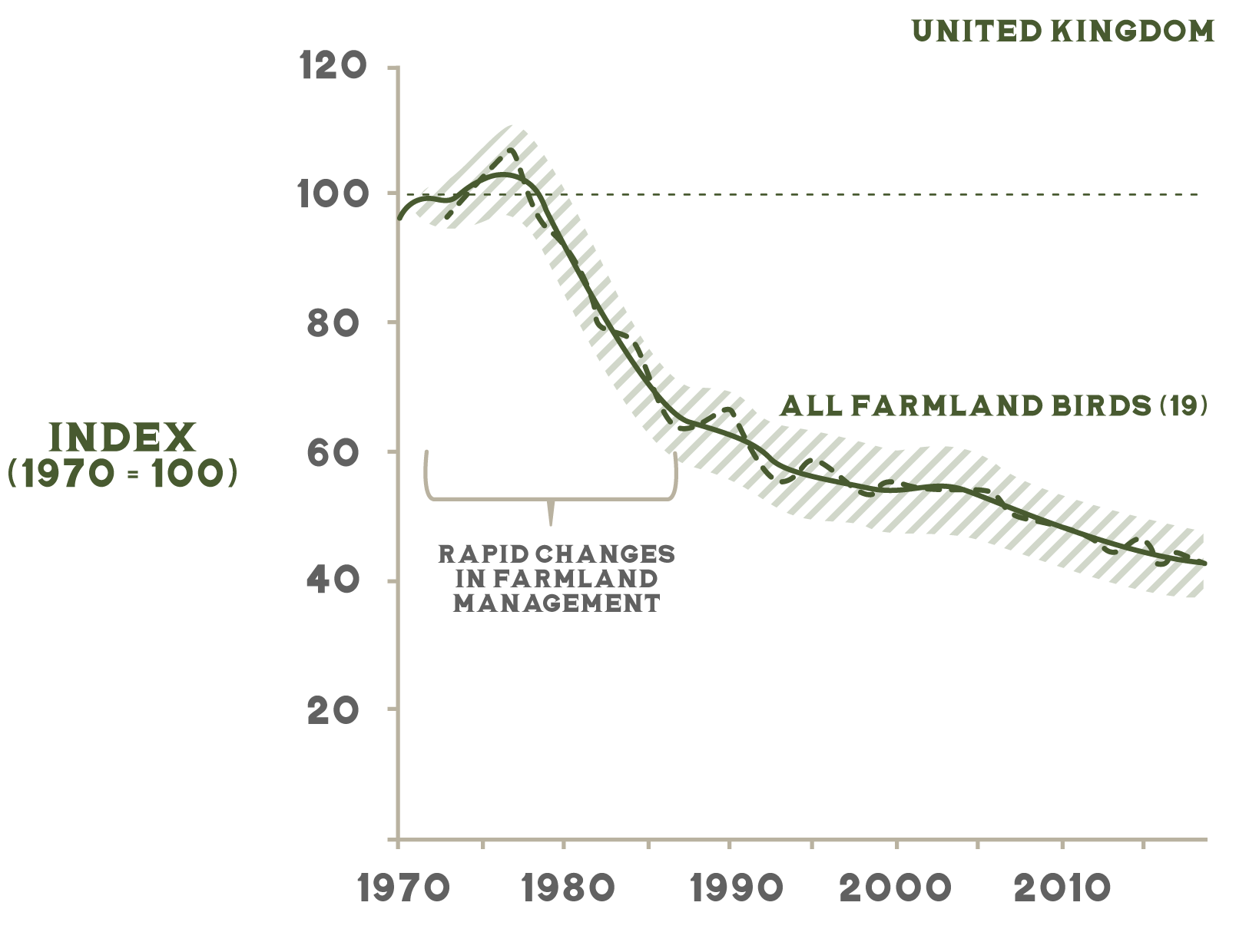
The suite of environmental changes that occur during agricultural intensification often have complex and hard-to-predict effects on organisms. In northern Spain, for example, if farmland shifts from non-irrigated to irrigated production, bird species richness declines an average of 24%. It seems that irrigation reduces the availability of nesting sites for many species in ways that seem subtle to non-bird eyes. Many farmland bird species like to nest in wheat and barley fields, but farmers who use irrigation often instead plant maize, which many species find unsuitable as nesting habitat.96
7.3 Constraints and Trade-Offs
Section 7.3: Constraints and Trade-Offs
We face an existential conundrum. We depend on our agroecosystems for our well-being, and that dependence will only grow as we strive to provide all people with the capacity to lead happy and fulfilling lives. But our agroecosystems radically alter the planet. So much so that they could help push planetary conditions past the point where most of us will be able to lead happy and fulfilling lives—at least in the ways that we have grown accustomed to defining those things. We have not thought about this fundamental trade-off over most of the time that we have been developing and tinkering with the design of our agroecosystems. That blind spot has played no small part in leading us down design paths that have intensified their detrimental influence.
We can do better. In Sections 7.4 and 7.5, I explore some of the ways that we are redesigning our agroecosystems to lessen their impact on the Earth System while enhancing the benefits they provide us. But before exploring the current strategies for optimizing the benefits and costs of agriculture, we should first consider some of the more practical constraints and trade-offs that we have to work through and around. These constraints and trade-offs are fundamental in the sense that they have always been around in various forms and to varying degrees. They form the landscape of possibilities that define the ways that agroecosystems could look and how they could function. But just like physical landscapes, they aren’t immutable. Technological innovations such as the Haber-Bosch process (see diagram as lightbox) can radically alter the landscape and create new viable design pathways. The same is true for changes to the basic characteristics of the Earth System such as its climate. It is also easy to go down one design path without recognizing that there are other paths just over the horizon that could lead us to very different outcomes.
There are two broad categories of these constraints and trade-offs.
Physiological Constraints and Trade-Offs
One set of constraints and trade-offs involve the physiological processes carried out by our domesticated organisms. Organisms capture energy and distribute it around to do various bits of work, such as growing, avoiding being eaten, competing against other organisms for resources, and reproducing. In an evolutionary sense, all that work is being done to increase the likelihood that the organism’s genes get passed on to future generations. Natural selection is remarkably effective at finding solutions to life’s problems, but while the solutions are effective, they aren’t perfect—at least from our perspective. A good example is photosynthesis. Even under the most ideal conditions, only about 2% to 4% of incoming light energy gets captured and converted into biomass by terrestrial crops.97 From our perspective of generating food, that is a significant bottleneck. Compared to other limiting resources such as land and nutrients, we have plenty of light. If we were able to increase the photosynthetic efficiency of our crops by just a few percentage points, it could dramatically increase food production.98 Breeders and biotechnologists have long sought to improve the efficiency of photosynthesis, spurred on by a few tantalizingly clear design limitations.
For instance, RuBisCO the enzyme that catalyzes the first key step in converting atmospheric CO2 into carbohydrates occasionally attaches itself to O2 instead of CO2, a process called photorespiration. The imperfect affinity of RuBisCO reduces the theoretically attainable maximum photosynthetic efficiency of C3 plants by 48%.99 Under more realistic field conditions, one study estimated that in 2016, photorespiration decreased wheat yield in the United States by 20% and soybean yield by 36%.100
Natural selection hasn’t been blind to the inefficiencies. C4 plants evolved a tweak for reducing photorespiration by pumping CO2 into specialized structures within leaves, allowing RuBisCO to work more efficiently under higher CO2 concentration. Crassulacean acid metabolism (CAM) plants maintain a high concentration of CO2 for RuBisCO in a different way. They open their stomata at night (the opposite time from other plants) and store CO2 as an organic acid. During the day, they keep their stomata closed and complete photosynthesis by regulating the release of the stored CO2. That trick not only maintains a high CO2 concentration for RuBisCO but also significantly reduces the water lost during photosynthesis since their stomata are closed during the heat of the day.
We have been able to tweak things on our own. New techniques such as gene editing have allowed us to manipulate the expression of a wide range of enzymes involved in photosynthesis. The ability to manipulate multiple genes has been a key advance. In the past, researchers could only practically adjust one or two steps in the long and complex biochemical pathways that directly and indirectly regulate photosynthesis. Changing one step of the process often just created more issues at other steps in the process. By simultaneously adjusting multiple steps, researchers have begun to produce better results. For instance, researchers simultaneously manipulated several genes involved in both the initial conversion of light energy into chemical energy (the light reactions) as well as the conversion of carbon dioxide into carbohydrates (the dark reactions, or the part that RuBisCO plays a role in). When grown in the field, the manipulated plants accumulated 27% more biomass than unmanipulated controls during the early part of the growing season.101
That sounds revolutionary, but reality is bit more disappointing. When researchers let the plants grow until they flowered and produced fruit (the typical time that we harvest most of our crops), the growth advantage of the genetically manipulated plants evaporated. The researchers aren’t sure exactly why, but one hypothesis is that the plants faced different conditions later in the year that created different issues and different needs, all of which negated the nominal improvement in photosynthetic efficiency. Indeed, natural selection has already been there, done that, and bought the t-shirt.
Both C4 and CAM pathways are such nifty innovations that they have evolved independently multiple times over the history of plants. Yet C3 plants are still around—in fact, about 85% of the plant species on Earth are C3. Why hasn’t this inefficient system been selected out? The answer is that C4 and CAM are inefficient in other respects; namely, they use more energy to run than the C3 pathway. In some circumstances, the benefits of reduced photorespiration and improved water use efficiency outweigh the costs of the increased energy needed to run the system. Warm or water-limited habitats put the C3 pathway at a disadvantage compared to C4 and CAM pathways because the effects of photorespiration increase with temperature. In cooler, less water-limited habitats, however, the less energetically costly C3 approach has a clear advantage. It is likely that most of our manipulations to the photosynthetic infrastructure of plants will result in similar trade-offs.102
Such trade-offs influence almost every aspect of an organism’s life. As an organism acquires traits and characteristics that make it good at one aspect of life, it tends to get worse at other aspects. This fact has fundamentally shaped our efforts to breed crops. As mentioned in Chapter 1, the green revolution—and the broader innovations of which it was part—more than tripled global crop yields from those of the early 1960s. It is tempting to think of that achievement as simply the result of breeding better crops. But the crops we developed were only better under a specific set of conditions that we could create for them. We bred crops that were exceptionally efficient at converting nutrients and other resources into the specific portion of biomass that we harvested. But the life history traits that were needed to do that job came with trade-offs that diminished the ability of crops to do other jobs. As described above, high-yielding annual wheat varieties have scrawny, ephemeral roots that are poor at capturing soil nutrients and preventing soil erosion (see Figure 7.13). That trade-off reflects the fact that plants have a finite amount of energy available to them. If more energy is put towards fruit, less of it can be put toward roots.
When we first domesticated crops, we were forced to develop relative generalists. For one thing, we couldn’t consistently provide our crops with enough nutrients, so they had to be decent at finding nutrients on their own. It also helped if they could hold their own against competitors and at least try to put up a fight against pests. But our increasing ability to ameliorate the stresses and challenges faced by our crops freed plant breeders to develop more specialized designs. In addition to having scrawny roots, modern wheat varieties have skimpy stems and leaves (Fig. 7.22). About half their aboveground biomass is in the form of grain.103 They are the plant equivalent of Formula One race cars—exceptional at going very fast in one direction but horrible at doing much else. For instance, the newer varieties have higher yields compared to the older varieties when grown under ideal weed-free conditions, but that advantage disappears when the varieties are forced to compete against weeds. In one study, newer wheat varieties suffered nearly a 45% reduction in yield when grown in the presence of a weed compared to only a 10% to 15% reduction for the older varieties.104 The green revolution was not just a revolution in breeding; it was the invention of a system that coupled specialized organisms with specialized environmental conditions. The increasing specialization of our domesticated organisms and the conditions that support them have created a whole other set of biodiversity mediated trade-offs.
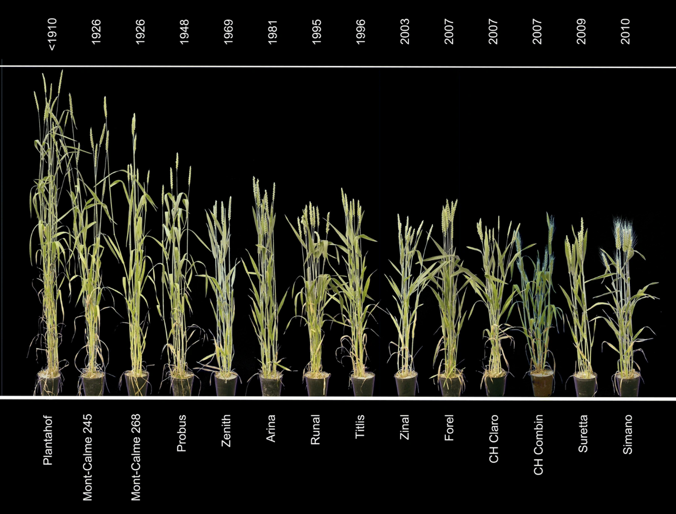
Specialization Reduces Biodiversity and Ecosystem Function
As described above and in Chapter 6, the relatively narrow and specialized conditions that we create for our domesticated organisms tend to reduce the overall biodiversity of agroecosystems. Creating and maintaining narrowly tuned conditions for a few crop species reduces the overall variability of habitat across space and time. The reduced habitat variability in turn restricts the niche space available for other organisms so that only a relatively small subset of species can regularly find suitable habitat in agroecosystems, particularly at the small scale of individual fields. On top of that, some of the conditions that we create to support our domesticated species are often acutely hostile to organisms that would otherwise find agroecosystems to be suitable places to make a living. The pesticide-associated declines in insects and farmland birds that I describe above are examples.
Agroecosystems with low biodiversity have low levels of a range of ecosystem functions and associated services. Figure 7.23 illustrates how that relationship is mediated through the specific ways in which we manage agroecosystems. It summarizes the results of more than 5,000 studies that evaluated how practices designed to increase the biodiversity of agroecosystems affected various ecosystem functions. The practices used in the studies included installing border habitat such as hedgerows, increasing the diversity of the crops grown, reducing tillage, and reducing the use of pesticides and inorganic fertilizer. Applying the diversification practices broadly increased a range of functions and services, including overall biodiversity. Many of these functions directly support the prime goal of agriculture: producing crops. Those results suggest that we are faced with rather perverse trade-off. The more we regulate environmental conditions to favor our specialized crops, the less diverse our agroecosystems become, and the fewer ecosystem services they generate to help us grow crops. Our general solution to that trade-off over the course of agro-industrialization has been to replace declining ecosystem services with our own intensive support systems: chemical fertilizers, chemical pest management, intensive tillage, and irrigation.
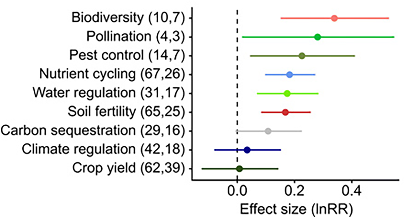
This trade-off is not necessarily one between biodiversity and agricultural yield. In Figure 7.23, the mean effect of diversification practices on yield is near zero, albeit with considerable variability. More biodiverse fields had the same average yield as less biodiverse ones. That suggests that we could potentially maintain high agricultural yields while supporting higher levels of biodiversity in our agricultural landscapes than we currently do. More biodiverse agroecosystems would in turn mitigate the broader impacts that agriculture has on the Earth System.
7.4. Improving Resource Use Efficiency
Section 7.4: Improving Resource Use Efficiency
Much of the environmental footprint of agriculture stems from the resources we use to run it. We use prodigious amounts of limiting resources like water, making them unavailable for other users in an ecosystem; we use inputs such as nitrogen and phosphorous inexpertly so that much of what we add ends up causing pollution in some other ecosystem; we use inputs like pesticides that come with substantial collateral costs. Using resources more efficiently is therefore a good place to start if we want to limit the environmental impact of agriculture. In Section 7.1, I described some of the metrics and tools that we can use to describe agroecosystems in terms of their resource use efficiency. Here I briefly describe some of the ways that we have approached improving the resource use efficiency of agroecosystems. There are several broad approaches.
Adjust Functional Traits
Just as we have developed crops that are good at converting resources into harvestable biomass, we could develop crops that are good at capturing and retaining resources within agroecosystems. Options that have been explored include developing perennial forms of annual crops, developing nitrogen-fixing cereals, and improving the water use efficiency of crops.105 But the trade-offs that produced high-yielding but skimpy-rooted crops also come into play if we try to produce more resource capture and retention efficient crops. For example, researchers have been trying to develop higher-yielding perennial forms of wheat-like grasses (such as the perennial wheatgrass in Figure 7.13). The goal is a plant that produces a decent amount of useable grain but that is also more resource capture efficient, better at resisting soil erosion, and better at contributing soil organic carbon than annual wheat. Researchers have been modestly successful, but it is impossible to get around the fundamental fact that more and deeper roots necessarily means less grain. Even the best new perennial wheat substitutes have grain yields that are typically far less than half that of annual varieties.106
That said, more resource-capture-efficient crops could be useful in some circumstances. For instance, their modest grain production could help diversify the revenue streams and overall portfolio of services in animal forage or biofuel feedstock production systems. In addition, we could make more modest tweaks to the allocation patterns of crops that wouldn’t cause such dramatic reductions in yield. These crop designs would be more like fancy sports cars instead of Formula One race cars. For instance, we could develop annual crops with slightly longer roots that fostered a bit more soil carbon sequestration or helped hold on to the soil a bit more. We could potentially tweak things so that reductions in actual realized yields were more modest than those of the perennial forms.
Another potentially transformative approach is to focus on the critical relationship between plant roots and fungi. It’s incorrect to view plant roots as simply being part of the plant. Roots are a plant-fungi amalgam. Without their relationships with mycorrhizal fungi, plants would be considerably less capable of capturing soil resources, surviving drought and heat, resisting pests and diseases, and competing with other plants. These relationships are as subtle and complex as they are important. The genetics of the fungi, the genetics of the plant, the composition and diversity of other species in the system, current environmental conditions, and even past environmental conditions can all interact to influence the consequences of the relationships for everyone involved.107 In agroecosystems, some combinations of crop varieties, strains of fungi, and conditions can increase the resource capture efficiency of crops and resource retention in the system as whole, while maintaining or even increasing crop yields.108109 But other combinations can just as easily be a net detriment to crops.110 Given how important these relationships are, it is surprising how little we have thought about them when designing agroecosystems. Many of our crop varieties are horrible at forming beneficial relationships with mycorrhizal fungi, and that is even before we consider the often inhospitable conditions we create for mycorrhizal fungi through the intensive use of chemical fertilizers, fungicides, and tillage. Researchers have just begun trying to develop crop varieties that are more sociable in their relationship with mycorrhizal fungi, as well as strains of mycorrhizal fungi that are more amendable toward crops under typical agroecosystem conditions.111
Precision Agriculture
One important strategy for improving input use efficiency is to more accurately apply inputs. In the case of resource inputs like nutrients and water, the aim is to deliver inputs in ways that allow more of what we apply to actually get taken up by the crop. In the case of pesticides, the goal is to ensure that most of the negative effects of pesticides affect the intended target and that there are limited collateral consequences. We have developed a number of tools and techniques to help attain those goals, collectively called precision agriculture.
Precision agriculture often makes use of advanced technology such as robotics and information technology. The advances we have made in more precisely meeting the water needs of crops provide a good illustration. One of the fundamental obstacles that precision agriculture tries to overcome is a lack of information. Divining the resource needs of crops has always been one of the most difficult aspects of farming. One challenge is that even in relatively homogenous agroecosystems, there can still be considerable variation in environmental conditions that create variable resource needs. Some parts of a field might have sandier soils and dry out more quickly than less sandy spots, creating spatial variation in water availability. Some parts of a farm might have different microclimates that create variation in crop water usage. And of course, water needs can vary from day to day and season to season depending on the weather. Historically, farmers have had coarse-scale information about environmental conditions on their farm and even less information about how those conditions translate into crop needs. For instance, many farmers get basic temperature and rainfall information about their farm from a weather station that might be located miles away and has experienced a markedly different set of conditions than those on the farm. Plus, how environmental factors such as temperature and rainfall translate into crop water need depends on the type of crop along with a host of other local-scale conditions such as soil type. Without detailed and specific information about water needs, farmers often apply water uniformly at rates that they hope will satisfy the thirstiest their crops might get. As a result, farmers often over-apply water, at least to some parts of their fields at some times. A range of new technologies are providing environmental information to farmers at increasingly finer scales of detail. Typical systems involve networks of relatively inexpensive sensors—sometimes deployed on unmanned aerial vehicles—that provide spatially detailed environmental data in real time. Information systems collate the data for use as inputs in ecological process models that predict crop water needs. The outputs are then relayed to farmers as recommendations about where, when, and how much water needs to be delivered on any particular day on any particular square meter of the farm.112
But it doesn’t help a farmer to know that one part of their field needs less water than another part if they don’t have a practical way of delivering different amounts of water. Another aspect of precision agricultural is focused on making resource delivery more precise. The simplest irrigation systems divert water from a source like a river directly onto fields along furrowed rows or sometimes just as a broad sheet. This type of flood irrigation is cheap and effective at getting water to the crop, but it is not particularly efficient. For one thing, a big slug of water flooding a field is too much for crops to handle all at once. As a result, much of the diverted water evaporates or seeps away into the groundwater before crop roots can suck it up. In addition, the flooding delivers water more or less uniformly across a field without regard to any spatial variation in the existing soil moisture conditions. We have progressively developed systems that give farmers much more fine-scale control over water delivery. One important innovation has been drip irrigation systems that deliver measured amounts of water at precise times near the roots of individual plants. We have also developed systems that can dynamically vary water delivery to match the spatial variation in the amount of water required.113
We have developed similar information and delivery systems for the other resources we use in agriculture. Precision systems can provide farmers with spatially and temporally detailed information about crop nutrient needs, crop health, and the risk of pest attack. Global Positioning System (GPS) and sensor-enabled farm machinery can adjust—at the scale of centimeters—nearly all the practices we use in farming to better match them to varying environmental or crop conditions. These include adjusting the amount and type of tillage across the different soil types and topography of a field, varying the planting depth and spacing based on soil and weather conditions, varying and optimizing the timing of harvest across a field, and precisely targeting the amount and location of pesticides and fertilizers.
Pesticide application is a good example of the directions these technological advances are heading. Smart sprayer systems combine environmental sensors, data processing and artificial intelligence software, and robotics to precisely vary when, where, and how much pesticide is applied to a field. Some systems can identify individual weeds and only spray them, not the crops or bare ground. Other systems even differentiate crop individuals that are infested with pathogens or insect pests from non-infested individuals. The most cutting-edge designs mount the systems onto autonomous vehicles that roam the fields (Fig. 7.24). These systems can significantly reduce the amount of pesticides that farmers apply and limit collateral exposure to non-target organisms. Even relatively simple systems can be effective. For example, a study conducted in California orchards found that a spray system that delivered pesticide only when a tree was detected and not in the space between trees reduced pesticide application by as much as 40% and the nontarget deposition of pesticide on the orchard floor by as much as 72%.114
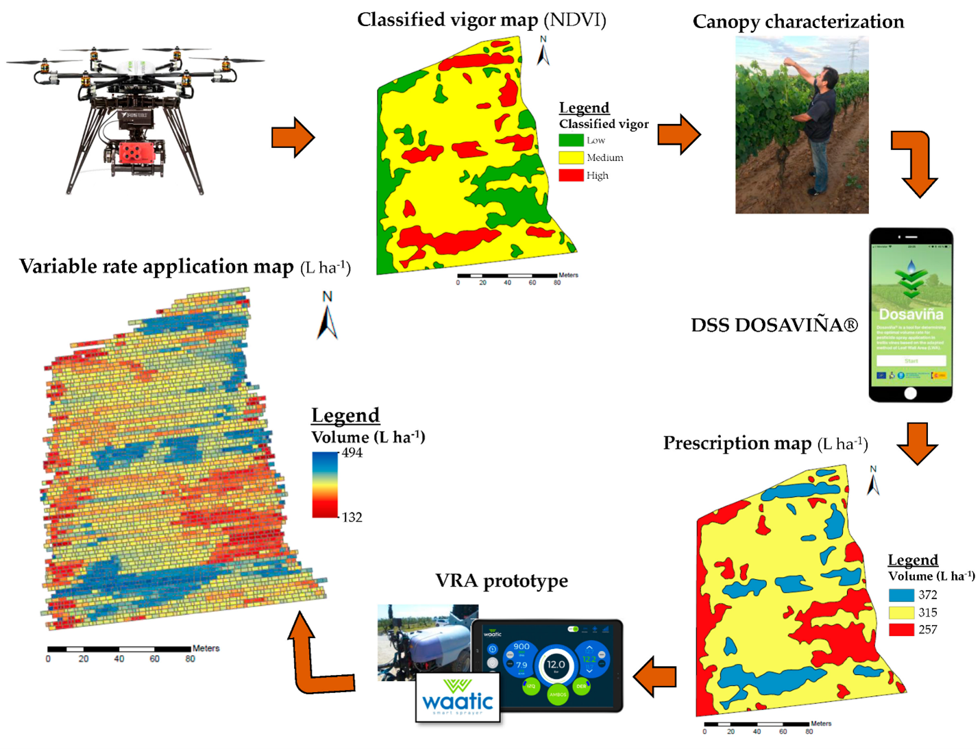
We can also more precisely use pesticides in ways that go beyond pesticide application. One example is developing chemical formulations of pesticides that are more narrowly toxic. We have made modest progress in that area, but there is only so far we can go toward making a chemical designed to kill some things but not others. The issues with the neonicotinoid class of pesticides mentioned above are a good example. Some emerging technologies offer the promise of much finer targeting, however. One is using pheromones and other signaling chemicals to disrupt the mating behavior of pests, known as mating disruption. For example, coddling moth (Cydia pomonella) is a major pest in apple and pear orchards. Its populations have been primarily controlled through the extensive use of broad-spectrum pesticides. But we can now synthesize the sex pheromone that male coddling moths home in on to find females. By flooding an orchard with the pheromone, farmers can sexually confuse and disorient the males, significantly reducing the number of successful matings and the resulting larvae that damage fruit.115 Signaling pheromones can be designed so that only a specific species or narrow group of species are influenced by them, and the chemicals are largely nontoxic at the small dosages needed, even to the organism they are targeting.
Another set of still largely conceptual ideas involve using emerging genetic engineering techniques as pest management tools.116 One example is RNA interference (RNAi), in which double-stranded ribonucleic acid (RNA) molecules inhibit gene expression. RNAi also more colloquially called gene silencing. In its proposed use as a pest management technique, RNA molecules could be designed to inhibit critical genes in target organisms and then sprayed on fields where they could be taken up by the target organism. Similar to pheromones, the silencing RNA would be designed to narrowly target a specific species or narrow group of species. Another potentially useful technique is the CRISPR-Cas‐9 gene editing system. CRISPR, short for clustered regularly interspaced short palindromic repeats, has a number of pest management applications, such as helping to more quickly and easily develop disease-resistant crops. One of the more provocative suggested applications for CRISPR is to deliver a gene drive that would allow a gene mutation (even a deleterious one) to rapidly spread through a population. For instance, we could introduce a deleterious mutation to a pest population, and it would rapidly spread on its own.117 Not surprisingly, the idea is controversial; you don’t need much imagination to come up with ways that introducing a nasty gene that spreads rapidly by itself through a population could go horribly wrong.
An important aspect of the technological advances associated with precision agriculture has been their progressively greater accessibility. Information that once was available only to large institutions with access to a satellite and a supercomputer can now be downloaded to an individual farmer on their mobile phone. The cost of locally deployed environmental sensors and delivery systems such as zoned drip irrigation has come within the financial means of many more farmers than just a few decades ago. But the financial obstacles to implementing precision systems are still formidable, even for relatively financially well-off farmers. For the poorest smallholder farmers, they are so out of reach that they might as well still be the realm of science fiction. In some cases, we are developing approaches that specifically address the constraints of smallholder farmers. In the Punjab region of India, researchers have developed region- and crop-specific models that predict crop nitrogen needs based on leaf color. They have translated this information into the form of a plastic color palette card that farmers can use to more accurately determine how much nitrogen they need to apply. Farmers can also access the information via their mobile phones. The trial use of this inexpensive tool significantly reduced the amount of nitrogen fertilizer that farmers applied to their crops while maintaining yields.118
Reduce Tillage
We have taken a similarly low-tech approach to more efficiently using tillage. In this case, the efficiency improvements come more from a shift in philosophy than from technological advances. Tillage was one of the first agricultural tools we invented, and it is still one of the most widely used. Prior to the agro-industrial revolution, however, the massive effort and sheer drudgery involved in tilling fields using farm animals or our own hands limited the amount of it we could do. That changed radically with mechanization, and ever since we have been on a tillage binge. It has taken us a while to recognize that along with the benefits that tillage provides come some significant costs, particularly given the vast swath of the planet that we now till. The disturbance caused by tillage kills many soil organisms directly, but even more importantly, it simplifies and homogenizes the physical habitat available for soil organisms (Fig. 7.25). This reduces soil biodiversity and the ecosystem services (such as pest regulation and nutrient cycling) associated with them. The warmer and more aerated conditions created by tillage increase decomposition rates, reducing soil organic matter and increasing emissions of greenhouse gasses from the soil. Those conditions also increase evaporation rates of water from the soil, reducing the amount that is available for crops. Tillage increases soil erosion by removing the protective cover of plant biomass that ameliorates the force of wind and water. Over time, frequent tillage can ironically cause many of the same soil problems that it is meant to alleviate. Initially, tillage creates a light, aerated profile of uniformly fine soil particles that is a wonderful place for a germinating seed. But over time, those uniform particles tend to pack closely together as they settle, forming a solid mass of soil with few air spaces. Heavily tilled soils often form crusts on top and hardpans below, usually right at the depth where tillage stops. In aggregate, all of those processes tend to reduce soil fertility. They also tend to lock farmers into a viscous cycle where they need to add increasing amounts of inputs to restore fertility and use ever increasing amounts of tillage to temporarily alleviate the negative physical conditions like crusts and hardpans that tillage creates.
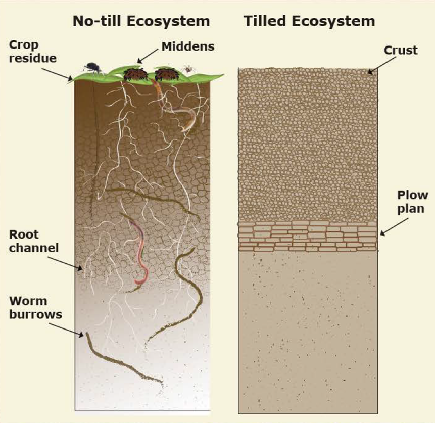
As we have better recognized those costs, we have started to use tillage more judiciously and in ways that maximize its benefits but that minimize the costs. Collectively, these strategies are known as conservation tillage. The name references the fact that many of the techniques were originally developed as ways to conserve soil by reducing soil erosion. The core idea is to leave cover crops or the non-harvested residues of previous crops in place and plant the new crop within that matrix using a minimum amount of soil disturbance (i.e., tillage). There are a variety of different techniques that vary in how much of the previous crop residues are left and how much of the field is tilled. Some of the more common techniques include planting seeds into individual holes drilled into the soil, tilling narrow strips of soil just where the seeds are planted (Fig. 7.26), and planting seeds on narrow ridges formed during the cultivation or the harvest of the previous year’s crop. These systems still provide the benefits of tillage but with far less actual tillage and far fewer collateral costs.
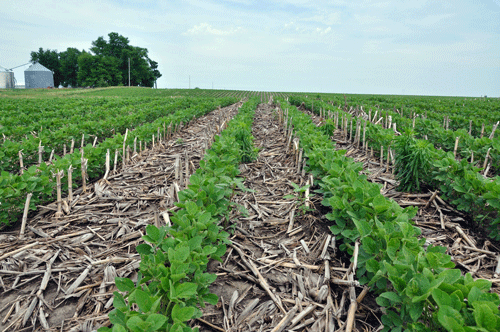
Integrated Pest Management
Like tillage, pesticides come with significant benefits as well as some profound costs. Optimizing that trade-off has become an important goal for our agricultural systems, although unfortunately that hasn’t always been the case. It must have seemed like a miracle of modern science when relatively inexpensive and effective pesticides became widely available to farmers after World War II. For the first time in history, farmers had a tool to stop a pending pest outbreak in its tracks. Instead of watching in horror as pests destroyed their fields, a farmer could proactively take action and within hours turn a pending catastrophe into a minor bump in the road on the way toward another bumper crop. We became mad with this power. If pesticides could be used to stop catastrophes, why not use them to keep pest abundance as low as possible or use them prophylactically, even before we saw the first signs of an outbreak? It took us a while to understand the why not.
First, we began to realize the serious environmental and human health costs of pesticides, research that was so eloquently summarized in Rachel Carson’s Silent Spring.119 But we also began to realize how a ham-fisted use of pesticides was often as counterproductive to growing crops as it was a help. Pest organisms quickly began to evolve resistance to our most commonly used pesticides, forcing us to switch to new ones or use the old ones at higher doses. Many of the pesticides we used also killed the natural predators of pests, which paradoxically also forced us to use even more pesticides that killed more beneficial insects and fostered the evolution of more resistance in the pests. This spiral of feedbacks is known as the pesticide treadmill.
One solution has been an approach called integrated pest management (IPM). One aspect of IPM uses the tools of precision agriculture to more precisely target only the individual organisms that are causing damage to crops. The approaches such as smart spray systems and mating disruption, described above, are important tools to help us do that. Another, more conceptual, aspect of IPM involves adjusting how we approach the use of pesticides in the first place. The basic idea is simple: only use pesticides to prevent pests from causing a significant level of damage. Like many things, implementing that simple concept can be easier said than done. For one, there are a variety of ways to define what significant damage is. The most common definition is the abundance of pests at which the economic damage they cause the farmer is greater than the direct cost of using pesticides to prevent the damage. There are always pests in our agricultural systems causing some amount of damage, but this is only a problem when they reach levels that are economically damaging to the farmer. The economic threshold frames the use of pesticides in efficiency terms: benefit gained relative to the cost. Using pesticides when pest abundance is below the threshold and not likely to cross it any time soon is economically inefficient.
In addition to helping farmers better target pesticide applications, technology advances are also helping farmers implement the threshold decision part of IPM. One of the most difficult and expensive parts of IPM is monitoring and predicting pest abundance so that farmers know when they are at risk of crossing an economic threshold. Automated decision support systems have been developed to help farmers do this. These use information on environmental conditions and pest abundance collected from regional networks of monitoring stations (and sometimes crowdsourced data) to parametrize mathematical models that can predict the trajectory of pest abundance down to the scale of local fields and particular days. This information can be delivered to a farmer’s smartphone while they are standing out in the field trying to decide whether to make a pesticide application.
Improving Food System Efficiencies
Growing crops is just one part of the broader systems we have developed for making use of those crops. These systems involve harvesting, storing, and transporting harvested crops; processing harvests into various products; trading the products in markets; delivering the products to consumers; making and eating meals; and finally dealing with the leftovers. When we are talking about the agricultural products we use to feed ourselves, these broader systems are collectively called the food system. The global food system is complex and shaped as much by socioeconomic conditions as by ecological constraints. It also has some obvious inefficiencies. Figure 7.27 maps out the flow of net primary production generated by our croplands and grazing lands. Only 6% of global agricultural production ends up in our mouths.120 Framed another way, we cause a lot of ecological impact for not a whole lot of human consumed food. There are a few main sources of the inefficient flow from field to fork.
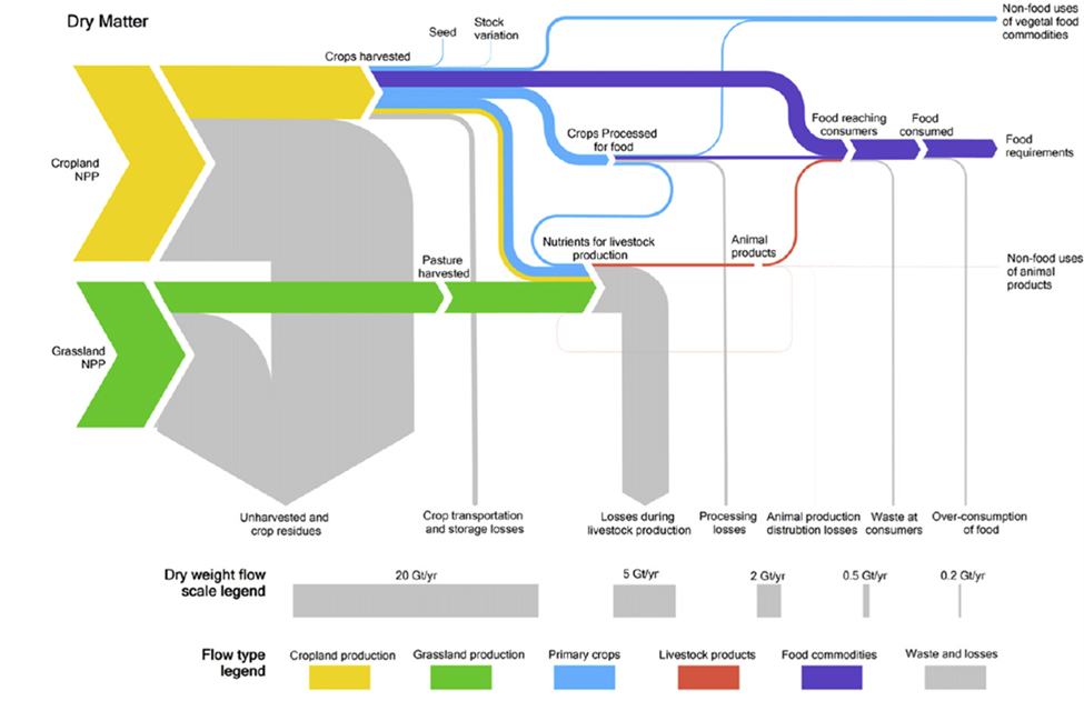
The biggest absolute loss in the food system occurs right at the beginning, during harvest, as indicated by the large downward pointing gray arrow labeled unharvested and crop residues in Figure 7.27. Some of that loss is caused by inefficient harvest—tomatoes that get squashed during picking or apples that are left on a tree. But a lot of it is related to a fundamental constraint: only certain parts of plants are edible, nutritious, or tasty. The rest—bits like roots and leaves—get left in the field. It is this inefficiency that caught the eye of plant breeders and spurred them to develop plant varieties, such as the annual wheat in Figures 7.13 and 7.22, that allocate a higher proportion of their biomass to the specific parts we want. But as I describe above, creating crop varieties that funnel more plant resources into edible bits comes with significant trade-offs, which themselves create inefficiencies in resource use and generate environmental impact. In the broad sense, much of the left-behind crop NPP probably shouldn’t be considered an inefficiency, but rather an investment in the stability and sustainability of the system as a whole.
The large amount of crop biomass left in fields distorts the perspective of Figure 7.27. All the subsequent losses of potential food look small by comparison. But we shouldn’t think of these losses as small. We can see why if we shift the frame of Figure 7.27 to just consider losses after harvest. Important postharvest losses stem from the trials and tribulations along the supply chain from field to mouth. Some supply chain losses happen when we process harvests into food products like a box of breakfast cereal or a bag of carrot sticks. A portion of the harvest also spoils, gets eaten by pests, or is otherwise damaged during storage and transportation. Significant losses also occur near the end of the chain—the moldy leftovers in the back of my refrigerator or the perfectly fine food that is tossed at the end of the night in a restaurant. Global estimates vary considerably, but roughly one-third to as much as one-half of the food that we harvest is lost to damage, spoilage, pests, or is otherwise wasted before we can eat it.121
Minimizing the attritional loss of food along the supply chain is more complicated than it might seem, partly because these types of losses often stem from complex socioeconomic factors that are context dependent. In poorer countries, much of the loss stems from inadequate supply chain infrastructure. Rudimentary postharvest pest management, poor roads, the lack of controlled environment warehouses, and the lack of refrigeration in the homes of many consumers contribute to large losses due to pests and spoilage. In richer countries, much of the loss happens just before consumption for reasons that have little to do with the lack of refrigeration or pest attacks. In the United States, roughly one-third of the available food is wasted before it is eaten, and roughly half of that waste happens at the consumption stage.122 The reasons include confusing labels such as “best used by” dates, strict food safety regulations, marketing gimmicks such as “buy one, get one free” deals, and the nuanced social factors that cause leftovers to mold in the fridge while takeout is ordered. As a result, even though the food supply chain has increasingly become globally integrated, minimizing its waste requires myriad local changes that involve entrenched socioeconomic complexities such as how many restaurant meals people eat per week or the reliability of a train that smallholder farmers take to market.
Despite the difficulties, reducing food loss and waste along the supply chain is a clear way that we can improve the human benefits provided by the food system while reducing its environmental costs. Improved efficiencies would economically benefit farmers, market sellers, and consumers, most of whom are smallholders or live near the margins of financial sustainability. Reducing waste could improve access to and the affordability of food for poor people. It could also increase the overall affordability of highly nutritious but also highly perishable foods such as fruits and vegetables, which are the most susceptible to food loss. Less food loss would also potentially mean that we would need to produce relatively less food, mitigating the environmental impacts associated with its production World.123
Some approaches to reducing food loss and waste use technological tools similar to the ones being used in precision agriculture. These include sensor-enabled automatic harvesters that cause less damage to the harvest and leave less of it in the field, radio-frequency identification (RFID) tracking technologies that improve the efficiency of food transportation networks, better monitoring of environmental conditions, packaging materials that improve the postharvest storage of food, and information systems that can more efficiently link the folks producing food with the folks eating it. As is the case with precision agriculture, technological innovations need to be developed that fit the constraints of smallholder and poor farmers. For example, affordable off-grid solar-powered cold-storage systems are being developed that could significantly reduce harvest losses for smallholder farmers.124 But many of the solutions to food loss will need to focus on economic and social drivers. For example, hermetic storage bags can significantly reduce harvest loss from pests, but because of their higher cost relative to more traditional storage systems, the economic benefits to smallholder farmers are less clear-cut, which significantly inhibits their use.125
Another significant inefficiency in our food system is related to the fact that we divert a significant portion of our crop NPP to livestock whose products (e.g., milk, eggs, steak) we then consume. The flow of energy and materials up through trophic levels is inherently inefficient (see Figure 3.4). For instance, only about 3% of the calories eaten by beef cattle gets converted into edible calories for humans.126 Other animal products have only slightly better calorie conversion efficiencies: pork (10%), chicken (12%), eggs (22%). You can see the scale of the trophic inefficiency imbedded in the food system in 7.27 (it’s the second-largest downward flowing gray arrow). Per year, 3.98 Gt of animal feed (from potential human edible crops like soybeans, forage crops like alfalfa, and pasture grass) are fed to animals to yield only 0.24 Gt per year of animal products, a 6% overall conversion efficiency. The inefficiency is exacerbated by all the directly human-edible crops that we funnel toward animals. In all, 36% of the calories we produce by growing crops (excluding the grasslands and forage crops we grow specifically for animals) is diverted into animal feed, 89% of which is subsequently lost before it is converted into animal-based food products.127 That makes meat production inefficient both in terms of resource use and environmental impact (see Figs. 7.9, 7.12, and 7.14).
Solutions for reducing the trophic inefficiency of the current food system are primarily social and economic, and they aren’t particularly straightforward. Eating more animal products has long been a symbol of prosperity. One of the things people do with newfound prosperity is to diversify and enrich their diets. As people moved out of poverty and into the global middle class during the Great Acceleration, it created a boom in the consumption of animal products (Figure 7.28). The numbers for poultry alone are staggering. Since the 1960s, the rate of poultry population growth has been faster than that of humans. In 2014, Earth was home (however briefly) to 23.4 billion poultry.128 For many of us, consuming meat and other animal products has become a small, attainable luxury that has improved our nutrition and quality of life. At the same time, for others, eating meat has shifted from being a luxury to being one of the cheapest and most accessible meals we can get on a daily basis. I have bought more than a few double cheeseburger value meals with loose change from around the house. In a feedback loop as destructive as the pesticide treadmill, as more of us could afford a bit of meat every once and awhile, the food system shifted to funnel more of the increasing crop yields into meeting (excuse the pun) the demand. As prices fell, it encouraged more of us to eat more meat, creating even greater incentive to produce it cheaper.
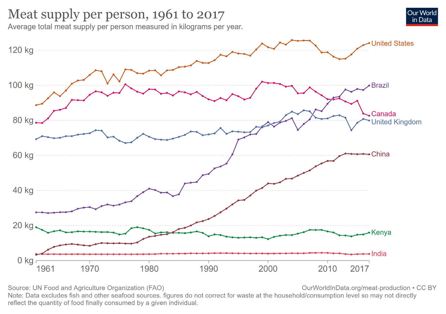
We shouldn’t think of meat consumption as only an individual lifestyle choice. Diet choices reflect complex social-economic interactions. As is the case with food waste, these interactions and their effects vary considerably across locations and communities. Evidence of this comes from an odd source: hair and fingernails. The isotopic composition of the keratin in our hair and fingernails provides a record of the food we eat. In the United States, researchers used samples of hair discarded from barbershops and salons to assess how diet varied with socioeconomic factors such as income. They found that poorer people ate a greater proportion of protein derived from corn-fed animals and less from fruits and vegetables than wealthier people.129 In poor and middle-income countries, however, similar isotope studies have found the opposite relationship: the consumption of animal-derived foods increases with increasing socioeconomic status.130 Creating societal shifts in something as wrapped in cultural identity and personal expression as diet may seem impossible. Still, the rapid explosion in meat consumption is itself a testament to how mutable diets can be. Given how much meat many of us currently eat and how trophically inefficient it is, even modest shifts in diet can have a big effect. Switching just 10% of daily caloric intake from beef and processed meat to fruits, vegetables, nuts, legumes, and selected seafood results in a 33% reduction in dietary carbon footprint.131
Reducing Yield, Knowledge, and Input Use Disparities
In Section 7.1, I describe some of the ways in which farms vary in their land and resource use efficiency (see Figs. 7.7 and 7.8). The efficiency differences are often related to differences in the socioeconomic environment experienced by individual farmers. In poorer countries, farmers may lack access to resources in all the senses of that word. Resources in the form of nutrient and water inputs, in improved locally adapted crop varieties, in the tools of precision agriculture, in locally relevant science-based agronomic information, and in supply chain infrastructure. These limitations conspire to create pronounced yield gaps, reduce the financial sustainability of smallholder farmers, and contribute to food insecurity. Narrowing yield gaps on the world’s least performing farms to just 50% of attainable yields could increase total food production by 8.5 × 10¹⁴ kilocalories per year, enough calories to meet the basic needs of about 850 million people.132
In more affluent countries, the problem is often paradoxically an overabundance of resources. This is particularly the case with nutrient resources. For many farmers in these countries, chemical fertilizers are relatively inexpensive, readily available, and easily fit into the rhythms and constraints of industrialized production systems. As a consequence, farmers often apply fertilizer at rates that put them way out on the plateau portion of the yield-resource input curve (see Fig. 7.7). Farmers are often not closely tuned to where they are on that curve because they get all of the marginal yield benefit (however small) of adding excess fertilizer but directly accrue almost none of the environmental costs, such as contributing to future climate change or nutrient pollution in a water body thousands of miles away. For these farmers, efficiency improvements will come from broader adoption of precision agriculture tools as well as from policies that create a stronger disincentive for excess resource use. In one sense, the industrialized scale of the problem is an advantage. Only three crops (rice, wheat, and maize) account for 58% to 60% of the global excess nitrogen and phosphorous applied to farmland. Given the fact that most of these farms are far out on the yield-resource input curve, nitrogen inputs could be reduced by 14% to 29% and phosphorus inputs reduced by 13% to 22% without causing any reduction in global grain yield.133
7.5 Ecological Intensification
Section 7.5: Ecological Intensification
One broad approach for reducing the environmental impact of agriculture is to design agroecosystems in ways that more explicitly use and take into account ecosystem processes and functions. As described in Section 7.3, the design of many of our agricultural systems has been shaped by an important feedback: we modify environmental conditions in ways that reduce biodiversity and associated ecosystem services; we then compensate for the loss of ecosystem services by modifying environmental conditions even further. All of that manipulation uses prodigious amounts of resources, comes with a range of broader environmental costs, and is often less efficient than the biological functions it is meant to replace.
We are beginning to develop more biodiversity-integrated agriculture using a variety of approaches and techniques. Many of these have been important farming tools for a long time and were more commonly used than they are today. Still, we shouldn’t think of these approaches as always involving a return to a simpler more bucolic form of agriculture, or think that they are only associated with particular types of farming such as organic agriculture. These strategies have been successfully integrated—at least on a limited basis—into even the most industrialized systems. This offers hope that we can ecologically intensify nearly all of our agricultural production. There are several broad approaches.
Create More Functionally Diverse Cropping and Animal Systems
Recall from Chapter 2 that complementary resource use, facilitation, trait uniqueness, and trait redundancy are the main mechanisms driving the positive relationship between biodiversity and ecosystem function. We can design mixtures of crop and species—polycultures—that leverage these mechanisms. Perhaps the best-known example is one of the great innovations of early Mesoamerican agriculture: the milpa (Figure 7.29). In a milpa system, multiple species of annual crops such as maize, beans, and squash are grown together or in close temporal succession. Fast-growing perennial crops such as banana are also often integrated into the system. The species used in the systems are chosen to have complementary resource use—such as nitrogen-fixing legumes and nitrogen-hungry maize, or to facilitate each other—such as the shade provided by banana plants.
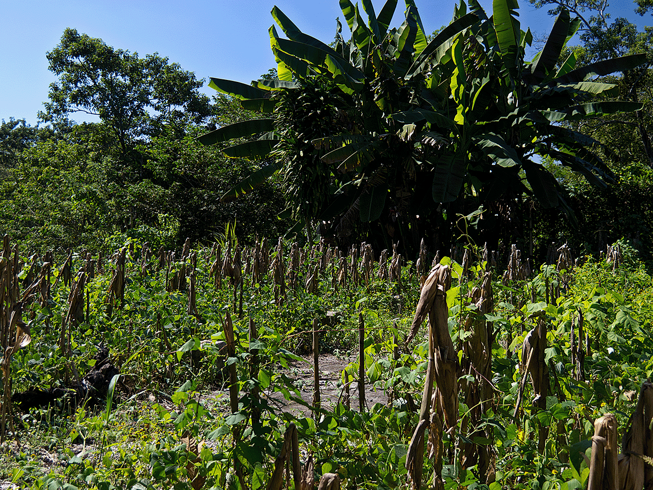
Polyculture systems can be land and resource use efficient. One measure of the relative land efficiency of polyculture is the land equivalent ratio (LER). LER is a measure of the degree to which the combined yield of a polyculture compares to the yield of growing each individual component separately as a monocrop:
[latex]LER=\frac{\text{yield sp1 in polyculture}}{\text{yield sp1 in monoculture}} + \frac{\text{yield sp2 in polyculture}}{\text{yield sp2 in monoculture}} + \cdots \frac{\text{yield spi in polyculture}}{\text{yield spi in monoculture}}[/latex]
Figure 7.30 works out an example for a typical milpa combination of maize, beans, and squash. Polyculture systems like milpas are still commonly used by smallholder farmers around the world, partly because they can provide a diverse range of food using a small amount of land. In the Western Highlands of Guatemala, nearly two-thirds of the farms are under the milpa system. The milpas produce more food per hectare and provide more of the recommended daily allowances of essential nutrients than mono-cropped maize alone.134 In addition, polyculture systems potentially provide a wide range of other benefits and ecosystems services, such as the ones listed in Figure 7.23.
| The Land Efficiency of a Maize-Bean-Squash Milpa | |||
|---|---|---|---|
| Crop | Yield in monoculture (kilograms per hectare) | Yield in polyculture (kilograms per hectare) | Polycultural Yield to Monocultural Yield Ratio |
| maize | 1981 | 1651 | 0.83 |
| bean | 710 | 288 | 0.40 |
| squash | 629 | 233 | 0.37 |
| Total Land Equivalent ratio | 1.60 | ||
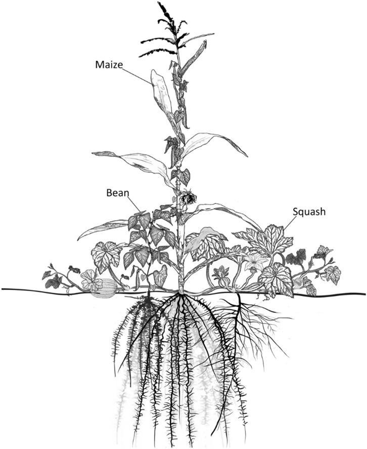
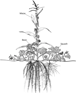
Similar benefits of complementarity and facilitation arise in mixed species flocks of livestock. For example, goats, sheep, and cows have different diet preferences. Goats mostly browse on shrubs, cows like grass and a few forbs, while sheep like a balanced diet of all three. This complementarity can convert more of the primary productivity in a plant diverse pasture into livestock biomass. A number of studies have shown that cattle and sheep raised together in mixed-species “flerds” (a portmanteau of flock and herd) can have as much as 24% greater yield than cattle-only systems.135 The animals in mixed-species groups are also often healthier and have less parasites than ones in single-species groups. Multiple species grazing can also maintain relatively high levels of plant diversity in pastures. For example, in the western United States, land that is grazed only by cattle tends to become dominated by shrubs (because the cattle don’t like to eat them), while land grazed only by sheep tends to become dominated by grass. Although sheep eat both grass and shrubs, the shrubs grow much more slowly than the grass, and they are more susceptible to sheep grazing. Grazing both cattle and sheep on pasture can create a more equitable abundance of shrubs and grass.
Polyculture systems are sometimes used in larger-scale and commercially oriented operations. The coffee and cacao agroforestry systems described above are examples (see Figure 7.3). But as I describe above, the general trend over the Great Acceleration has been to develop more specialized and less diverse cropping and livestock systems (e.g., Figure 7.18). Incorporating more diversity into these types of systems involves some significant challenges. For instance, complex mixtures of crops with different shapes, maturities, and harvest requirements are not amenable to mechanization. Similarly, each species of livestock has its own specific husbandry requirements that necessitate specialized equipment and expertise. Sometimes farmers can get a particularly good price for one or two of the species in a polyculture, and that can create strong economic incentives to maximize individual yields in monoculture. But there are several approaches to integrating the benefits of polyculture into these types of systems.
Modestly Spatially Separating Species
Depending on the species and particular functions involved, it is sometimes possible to get some of the benefits of facilitation and resource complementarity while modestly separating species within a field. The spatial separation can make it easier for a farmer to treat each crop differently in terms of things such as planting date and harvest. The separation can also make it easier to use machinery. One strategy of this type is called strip intercropping, where different crops are separated into strips consisting of several rows that are large enough to be worked independently by farm machinery. The relative proximity of the species can still be enough to gain yield and other benefits over completely separate monocrops.136 We can also play around with the spatial arrangement of multiple crops to get pest management benefits. Examples are trap crops that are more attractive to a particular pest species than a companion crop. The companion crop is usually either more susceptible to pest damage or has a higher economic value than the trap crop. The trap crop can be planted away from the more valued or susceptible crop—into a trap! For example, lygus bug (Lygus hesperus) is a serious pest of cotton, severely damaging the young developing cotton bolls with its piercing mouth parts. But lygus bugs also love a range of other crops like alfalfa, where they do considerably less damage. These alternate crops can be planted as a border around cotton fields to attract the lygus bugs and keep them out of the cotton during the critical boll development period. The J. G. Boswell Company (see the introduction to this chapter) used this approach on an epic scale by ringing their 80,000 acres of cotton growing in the bottom of former Tulare Lake with a lygus trapping buffer of alfalfa.137
Increase Intraspecific Diversity
In some cases, it is possible to create populations of crop species whose individuals have similar agronomic traits (e.g., planting depth and time to maturity) but that are complementary in other functional traits such as environmental tolerances, resource use patterns, or resistance to pests. These designed genetic mixtures can be managed in much the same way as genetic monocultures, but they have aggregate benefits over monocultures that include higher yields, higher yield stability in the face of environmental stresses such as drought or pest outbreaks, and improved input use efficiency.138 For example, in an experiment conducted in Hebei Province, China, plots grown using combinations of wheat cultivars that varied slightly in morphological traits such as root:shoot ratio, leaf area index, and height produced consistently higher yields and had greater water use efficiency than plots grown as cultivar monocultures. In that case, it seems that part of the benefit came from the fact that the mixtures had a more structurally complex and variable canopy that was more efficient at capturing sunlight than cultivar pure stands where leaves were more likely to overlap, causing competition for light.139
Crop Rotations
By far the most common approach to gaining the benefits of complementarity and facilitation is to link species in time instead of in space, that is, crop rotations. Although milpas may seem a universe away from the vast industrial maize and soybean mega farms of North America, both systems intercrop maize and legumes, one in space the other in time. The ecosystem services provided by crop rotations include yield benefits, reduced pest pressure, improved soil fertility, reduced soil erosion, and reduced nutrient leaching. These benefits can be achieved even in the most input-intensive cropping systems. In Illinois, maize grown as part of a sequential rotation with nitrogen-fixing soybeans has consistently higher yield than maize that is repeatedly grown on the same plot year after year. Maize in rotation also needs significantly less nitrogen fertilizer than continuously grown maize.140 As beneficial as the maize-soybean rotation is, it is still an extremely simplified system that is exacerbated by how ubiquitous it has become. In the grain-growing regions of the central United States, at least 90% of the 55 million ha in agriculture is composed of maize and soybean; roughly 30% of that acreage has been planted to just maize or soybean for at least two consecutive years.141 The benefits of crop rotations increase with the complexity of the rotation system in terms of the number of species used and the number of distinct stages in the rotation. A meta-analysis of 11 long-term rotation experiments found that maize yields are an average of 28% greater when grown in a diverse rotation than when grown continuously or as part of a simple two-species rotation. The diverse rotation systems are particularly good at maintaining yield during stressful periods such as drought, and they increase the probability of having a bumper crop during benign years (Figure 7.31).
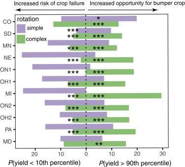
Some of the constraints and difficulties associated with spatially mixed polyculture systems also apply to rotations and some of the spatial separation approaches. For example, a farmer might need unique sets of equipment to plant, harvest, and store each of the crops in a rotation. Also, each crop in a rotation has a different economic return in the near term. Sometimes, one crop in the rotation is particularly valuable, which creates strong incentives for farmers to plant the most valuable crop year after year. Rotations can also be technically tricky to implement. For instance, in temperate regions, it can be difficult to harvest one crop in a rotation before seasonal weather conditions make it impossible to plant the next species—usually an overwintering cover crop. Some solutions to these challenges are technological. One solution to the challenge of using cover crops in temperate regions is to plant the cover crop into the field while the main crop is still growing, a technique known as inter-seeding. In these systems, precision farm machinery is used to drill seed the cover crop at the same time that fertilizer or weed control is being delivered to the main crop. By the time the main crop is harvested, the cover crop is already well established. Other solutions will likely involve short-circuiting the incentives that have been driving crop specialization over the Great Acceleration. These include policies such as taxes, rebates, and regulations that reward farmers for diversifying their cropping systems.
Integrating Plant-Animal Systems
The shifts in the food system that allowed the production of inexpensive animal products included spatially separating animal and crop production, focusing on single-species animal husbandry at large spatial scales, and deriving more of the feed we gave animals from cultivated crops instead of from grass in pastoral systems. Those practices neuter many of the ecosystem functions that animals provide. The separation of what is usually a close spatial trophic connection between animals and plants is one of the main factors contributing to nutrient pollution (see Figure 7.14).
In contrast, spatially integrated animal-plant systems provide a range of biodiversity-related benefits in much the same way that diverse cropping systems do. Putting crops and livestock in close proximity is an efficient way of recycling animal wastes back into more crop production instead of causing pollution in other systems. Because of their nutrient-recycling properties, many integrated crop-animal and pastoral systems require few—if any—outside inputs. Integrated systems can also be land use efficient, partly because livestock can convert forms of primary production that are indigestible or of low-quality human food—like grass or leftover crop stubble—into highly human nutritious food. During the early days of agriculture, domesticated animals were key tools for increasing the efficiency of agriculture in terms of converting farming effort and available land into human available calories. Livestock can also provide pest management services. For example, free-range chickens and geese can help manage insect pests and weeds in apple orchards.141 Under some circumstances, free-ranging livestock can even sometimes help support relatively high levels of plant species diversity. For example, moderate livestock grazing increases the plant species richness of California vernal pools and the pastures they are part of. This happens because livestock reduce the abundance of competitively dominant plant species, allowing other less dominant species to persist.142
While many farms—particularly smallholder operations—still closely integrate crops and animals, the global trend over the Anthropocene has been in the other direction. The causes are similar to the ones that have driven specialization within crop and livestock operations. Large single-species operations have efficiencies of scale that make their products cheaper and often more profitable to produce. The equipment and skills needed to raise animals are often different than the ones needed to raise crops. Grazing large herds of livestock on grass requires considerable amounts of land, which has tended to push grazing to remote lands that are marginal for crop production. That has exacerbated the spatial separation between crops and grazing.
Still, there are a few approaches for better integrating animals into even relatively industrialized crop production systems.
Integrated as Part of a Rotation System
Perhaps the most common technique is to forage livestock on fields during parts of a rotational cycle (Figure 7.32D). Often the livestock feed on a cover crop, but they can also feed (at least for a period) on main cash crops. Many farmers in the Southern Great Plains of the United States graze cattle on young wheat fields in what are called dual-purpose wheat systems. The grazing diminishes wheat yields a bit, and in fact the practice is another contributing factor to the yield gap experienced by wheat farmers in the region mentioned in Section 7.1. Although they slightly reduce wheat yield, the cattle provide an important economic hedge against more catastrophic crop losses in those fickle years when early-season heat stunts wheat fruit development.144
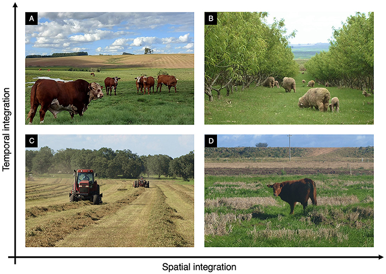
Periodic Use in Perennial Crops
Livestock can be periodically allowed to forage the understory of perennial crops such as orchards (Figure 7.32B). The livestock get access to a food source while reducing the abundance of weeds and insect pests in the orchard understory. Livestock can also redistribute nutrients across an orchard.
Cooperative Coordination
The folks growing crops and husbanding livestock in integrated crop-livestock systems don’t necessarily have to be the same people. By cooperating, separate crop and livestock operations can get some of the benefits of both specialization and integration. For example, a poultry operation could contract with tree fruit operations to periodically supply birds for pest management. In some cases, cooperation can create a measure of integration even if the crops and livestock remain spatially separated. For example, farmers can provide forage to a livestock operation in exchange for manure (Figure 7.32C). But these arrangements need to involve close coordination between the separate operations to avoid the pitfalls and inefficiencies associated with spatial separation (e.g., Figure 7.14). Having crop and livestock operations close together within the same region helps with the integration.
Landscape Diversification
As I mention in Section 7.4, agricultural landscapes have tended to become more homogenized both as a result of the loss of crop diversity as well as from the loss of species-rich habitat types such as perennial grasslands. Maintaining these more diverse habitats within farming regions can be a way of better integrating crop and animal production. The cork oak agro-silvo-pasture landscapes of the Mediterranean basin are examples of this type of integration (see Figure 6.8). Crops and livestock don’t necessarily have to be closely integrated on the same plots for there to be benefits. For example, pollinator-dependent crops grown adjacent to native grasslands can have enhanced pollination because the grasslands provide habitat for a diversity of mobile pollinators. The grasslands can also be used to support livestock (Figure 7.32A). I return to the topic of landscape diversification below.
Aquaculture
Many forms of aquaculture spatially integrate animals and crops. Perhaps the most historically important and still widely used example is the practice of raising fish in flooded rice paddies. Like the Mesoamerican milpa, farming rice and fish together was one of our great agricultural innovations. The rice paddies provide a protected habitat for the fish while the fish fertilize the rice with their wastes, provide pest control services, and help aerate the soil. In southern China, rice-fish systems require 68% less pesticides and 24% less chemical fertilizer than rice-only systems.145 A wide range of variations on the basic concept are practiced throughout the world’s rice-growing regions, including outside of Asia. Many of these are traditional designs that often simply involve a system for letting wild fish and other aquatic animals naturally colonize the flooded fields. The aquatic animals typically aren’t provided much in the way of supplemental food, and their natural stocking density is relatively low in these types of systems. More intensive designs have been developed that stock the aquatic animals at much higher densities and feed them larger amounts of supplemental food. These designs also often intentionally match compatible rice cultivars with specific fish species and breeds. They may rotate fish and rice cultivation across time instead of integrating them in space. These more intensive systems can retain many of the benefits of the traditional systems, such as reduced pesticide and fertilizer use while producing much higher yields of fish and net higher incomes to farmers.146
Even more intensive adaptations of the concept are the various examples of aquaponic systems that circulate water from the grow tanks of aquatic animals through biological filters that remove wastes. Sometimes the biological filter is a hydroponically growing crop (usually vegetables), but it can be other things such as microbial mats or even constructed wetlands. Nutrient and water recycling is the main ecological advantage of these types of systems.147 Another emerging form of intensively integrated aquaculture is integrated multi-trophic aquaculture. Most of the current research examples come from marine aquaculture. Marine aquaculture is an increasingly important source of the protein we eat and a way to reduce the intense pressure on dwindling wild fish stocks. But many marine aquaculture systems have notorious pollution and other environmental concerns. There is perhaps no clearer example of how we have short-circuited nutrient cycles than by feeding maize and soybean-based feed to penned fish in an ocean. As much as 85% of the phosphorus, 80% to 88% of the carbon, and 52% to 95% of the nitrogen contained in aquaculture feed is not taken up by the target fish.148 Integrated multi-trophic aquaculture attempts to create systems that are based on natural trophic connections so that the wastes and uneaten food of one species are used as food or nutrients for another species. A typical design combines fish such as salmon, macroalgae such as seaweed, filter feeders such as mussels, and deposit feeders such as sea cucumbers. The fish generate organic and inorganic wastes from their feces as well as from stray bits of uneaten feed. The macroalgae uptake dissolved inorganic nutrient wastes. The filter feeders consume tiny bits of uneaten fish feed as well as microalgae that may increase in abundance because of the elevated nutrients. They also consume the planktonic life stages of many disease organisms as well as viruses and bacteria, and they could therefore help reduce disease pressures on farmed fish as well as reduce the risk of transmitting diseases to wild populations. The deposit feeders consume larger bits of undigested food and wastes that sink down to the bottom. All of these elements are commercially harvested. One idea is to place these systems farther offshore, away from sensitive nearshore aquatic habitats such as estuaries and wetlands. Concept designs include integrating the offshore aquaculture with other infrastructure such as those for offshore wind farms. Since such remote spots would be lonely and inhospitable places for humans to live, autonomous vehicles and other robots could provide much of the labor-intensive work such as feeding and harvesting.149
Ecological Pest Management
Many of our farming practices foster conditions that make it difficult to manage pests. Crop monocultures based on yield-optimized varieties with poor defenses are susceptible to catastrophic pest outbreaks. Low levels of plant diversity on farms and in the surrounding farm landscape provide poor habitat for a range of organisms that act as natural enemies (predators, parasites, parasitoids, pathogens) of pests, which help to regulate pest populations and provide biological control of pests. Pesticides also directly kill or incapacitate natural enemies, further reducing the level of biological control on pests. All of those factors foster boom-and-bust cycles of pest abundance that are difficult to manage below an IPM threshold.
The net result is that we are not terribly good at pest management. Globally, on average, we lose 30% of our major crops like maize, wheat, and cotton to pests (insects, weeds, and pathogens), with losses approaching 80% in some regions.150 Remarkably, that percentage loss hasn’t changed much over the past hundred years—despite advances in technology and an increasing intensity of pest management. One reason is simply that we can’t stop evolution by natural selection. Our agricultural systems are intense crucibles of natural selection that generate a constant parade of new traits and strategies that allow pests to thwart our best defenses. But another equally important reason is that our pest management efforts have largely replaced biological pest regulation, not added to it. In fact, it is remarkable that we have been able to maintain a decent level of pest regulation given that we have otherwise designed agricultural systems in ways that make them extremely vulnerable to pests and that foster wild swings in pest abundance. We have been running simply to stand still. This might be a tolerable state of affairs if pesticide use did not also come with a range of other profound costs to ecosystems and our own health. In addition, the factors that contribute to the pesticide treadmill suggest that relying heavily on pesticides is a biologically unstable and risky strategy that contributes to a spiral of diminishing returns and increasing costs.
Reintegrating ecological pest regulation into our agroecosystems could reduce the broader societal and ecosystem costs associated with pesticide use, mitigate the effects of pests evolving ways around our defenses, and even perhaps produce broad improvements in the degree of pest regulation that we can achieve. There are two broad approaches to enhancing the natural pest regulation within agroecosystems. The first is to use integrative pest management (see Section 7.4). More efficiently using pesticides that are precisely applied and that narrowly affect just the target pests can greatly improve conditions for natural enemy species. The second approach is to increase the biodiversity of agroecosystems.
Pest regulation is one of the benefits associated with increasing biodiversity (see Figs. 2.13 and 7.23), partly because crop mixtures tend to slow down the spatial spread and population growth of specialist pest and disease organisms. For instance, the western corn rootworm (Diabrotica virgifera virgifera) is a maize specialist. Adults feed on maize leaves and flowers, while larvae feed on maize roots. A monoculture maize field is therefore a heavenly habitat for corn rootworms, and that heavenly habitat often stretches across large swaths of the landscape. The only reason that corn rootworms don’t chew their way through all the millions of acres of maize planted in the United States each year is that we use prodigious amounts of pesticides. These are incorporated into the soil, sprayed on maize plants, and integrated into the physiology of maize itself in the form of transgenic varieties that express insecticidal proteins from the bacterium Bacillus thuringiensis. But the ability of corn rootworm populations to rapidly grow and spread is considerably curtailed in systems where the maize is intermixed with species that don’t provide rootworm habitat, such as the beans and squash in a milpa, or in landscapes where maize fields are patchy and intermixed among non-crop habitat or fields planted to other crops.
Another reason for the positive association between biodiversity and pest regulation is that the natural enemies of crop pests benefit from the diversity. Natural enemy species require a variety of different resources and habitat conditions that are often in scant supply within low-diversity agroecosystems. Most predators, parasites, and parasitoids have at least modestly broad diets that include several species over the course of their life spans. Some species (such as many parasites) even require specific sequences of species to complete their life cycles. In biologically simplified agricultural systems, natural enemies often can’t find suitable prey or hosts during at least part of the year. This forces them to migrate away from fields, or it fosters wild boom-and-bust cycles in natural enemy abundance. Many species also require nonanimal food such as pollen and nectar, at least during some life stages. For example, adult parasitoid wasps feed on nectar. But agroecosystems often have a low abundance or diversity of flowers. Natural enemies also need specific physical habitat conditions, such as a patch of shade during the hottest part of the day, shelter to spend the winter or hide from their own predators, or a perch site to scan for prey. These also are often in short supply in homogenous agroecosystems.
There are a number of ways to increase agroecosystem biodiversity with the goal of enhancing pest control. Collectively, these are called conservation biological control, although the approaches often involve as much active planning and manipulation as they do conservation. These include the general approaches for diversifying cropping systems described above, such as the various techniques of intercropping, crop rotations, integrating crop and animal production, reducing tillage, and diversifying the types of crops grown across an agricultural landscape. Farmers can also specifically manage habitat for the natural enemies of crop pests, either at the scale of individual farms or across larger landscape scales. In some cases, this can simply involve being more cognizant of the potential habitat that already exists. Potential natural enemy habitat includes non-cropped borders of farms such as the edges of fields and the shoulders of roads, the understory vegetation of orchards, and perennial hedgerows that mark field boundaries (Figure 7.33). These bits of less managed habitat can provide important resources for natural enemies as well as a broad range of other species.151 For instance, the relatively undisturbed grassy edges of vegetable fields in western Oregon are where predatory ground beetles spend the winter. In the spring, the beetles move into adjacent fields where they provide pest control services.152

Farmers often manage the margins of fields almost as intensively as they do fields themselves to prevent the areas from becoming refuges for weeds and animal pests. Not only does that management contribute to overall reductions in biodiversity, but in some cases, it can also result in direct negative consequences to farmers. An example comes from sunflower fields in the Central Valley of California. Birds such as European starlings (Sturnus vulgaris) are major pests of the sunflower crop, and farmers tend to get rid of anything that might make their fields even more attractive to birds, like adjacent woody vegetation. At the same time, birds potentially provide biological control of another major sunflower pest, the sunflower moth (Homoeosoma electellum). Researchers conducted a field study to find out what the net result of having woody vegetation adjacent to fields was in terms of the pest control and pest damage provided from birds. As expected, the researchers found that there was a significantly greater abundance and diversity of birds along field margins that had woody vegetation compared to field margins that were bare or had herbaceous vegetation. But the greater abundance of birds in the woody margin fields didn’t translate into any greater bird damage compared to the non-woody margin fields. In contrast, the pest control of the sunflower moth provided by the birds was significantly greater in the woody margined fields. Moth damage was nearly four times higher in non-woody margin fields compared to woody margined fields. In monetary terms, losses from moth damage were $877 per ha in fields without a woody margin compared to only $220 per ha with one.153
Farmers can also actively design and create habitat that specifically supports the natural enemies of crop pests.154 The designs typically combine plant species that provide the resources needed by arthropod predators and parasitoids such as nectar, alternate prey, and physical cover. The plantings can take the form of marginal strips, form part of a rotational or intercropping system, or form the understory of perennial crops. They can be temporary, like an annual flower strip, or they can be more permanent, such as a perennial hedgerow. Figure 7.34 gives some examples. These intentionally functional designs are intended to generate the specific services farmers desire, for example, pest regulation. A study conducted in the Central Valley of California found that specifically designed hedgerows attracted more beneficial insects than pest insects, while adjacent unmanaged weedy areas attracted significantly more pests than beneficials.155 The design and composition of habitat plantings can be adjusted to fit specific pest control needs and management constraints. Researchers in Switzerland developed mixes of annual plant species that are attractive to and provide resources for the natural enemies of aphids that are major pests in the region. The plant species were chosen to have staggered flowering times so that floral resources are consistently available to natural enemies over the course of the entire season. Farmers can easily plant the mix using standard equipment and as part of their regular farm plan. The flower strips can be positioned along field edges or integrated into the field itself in a form of strip intercropping. The researchers found that potato fields with the designed flower strips had significantly higher numbers of natural enemies such as hoverflies (Syrphidae) and lacewings (Chrysopidae), resulting in 75% fewer aphids in flower-augmented fields compared to fields without flower strips.156
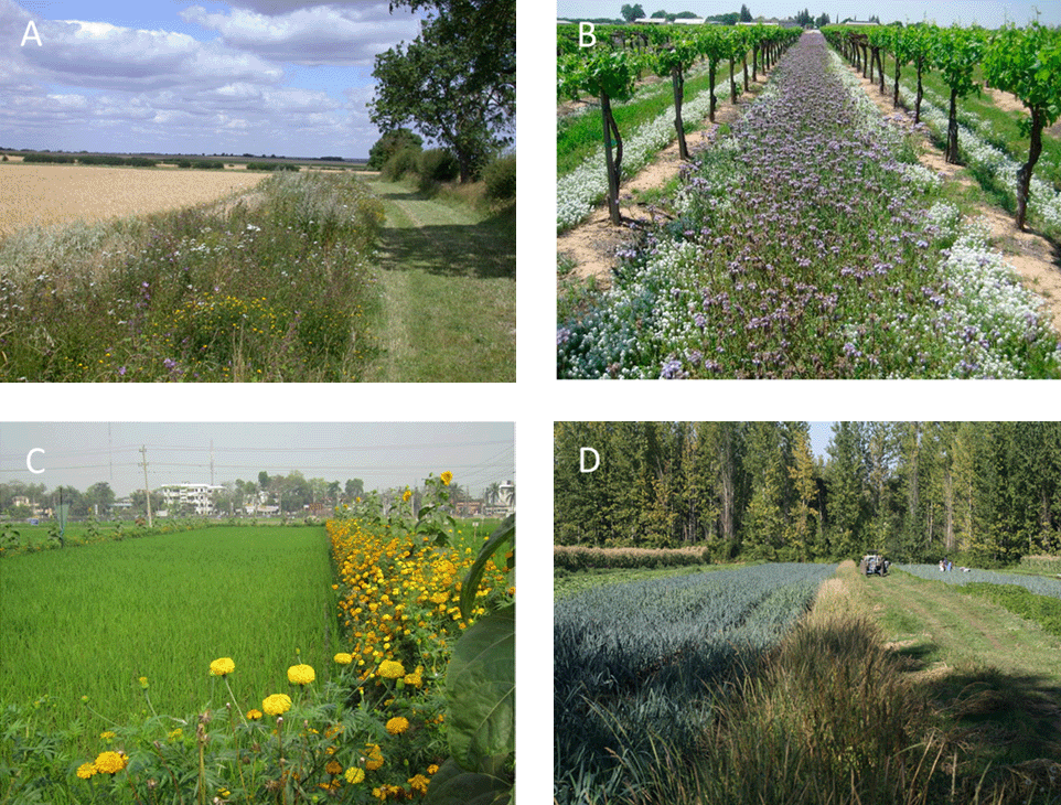
Overall, there is strong evidence that maintaining and augmenting these types of habitats in agroecosystems can significantly enhance populations of crop pest natural enemies and create measurable pest regulation services for farmers.157158 Still, there are challenges to getting more farmers to adopt these approaches. One issue is related to the fact that many natural enemies are highly mobile. As a result, their abundance and the level of pest control they provide at the local scale of a field are strongly influenced by conditions across entire landscapes, not just the local fields and farms that individual famers have direct control over. For instance, one farmer’s carefully planned beneficial insect habitat may go for naught if all the neighboring farms still prophylactically use broad-spectrum pesticides that kill natural enemies. In addition, mobile predators and parasitoids need access to habitat across a landscape so that isolated individual patches of habitat adjacent to an individual field may provide limited benefit if habitat conditions elsewhere across the surrounding landscape are generally poor. Studies testing the impact of adding on-farm habitat have found that the results are strongly influenced by conditions in the broader landscape. When researchers added hedgerows to the edges of grain fields in Italy, for example, it had no measurable effect on the level of pest regulation or pollination in the adjacent fields. It was only when multiple farms had hedgerows linked into a network of habitat across a landscape that measurable benefits occurred, and those benefits were measurable at the scale of individual fields. Fields in hedgerow-abundant landscapes had up to 18% more aphid parasitism and up to 70% more pollinator visitations and crop seed set than fields in hedgerow-scarce landscapes.159 Also, the level of pest control often declines with distance from habitat, so that pest control from natural enemies can be high along the edge of field but negligible in the center of it, particularly when fields are large. Overall, we don’t have a good understanding of spatial relationships of natural enemy populations and how those translate into pest control across landscapes. That hampers our ability to provide farmers with practical advice, such as what proportion of their farm needs to be in habitat and in what spatial configuration to optimize pest control.
Another complication is related to the inherent variability and complexity of biological systems. Even if natural enemies have access to good habitat across a landscape, their abundance can still vary over a season or from year to year because of any number of environmental disturbances and perturbations like the weather. Also, the connection between the abundance of natural enemies and the service of pest regulation can be murky and convoluted. For example, strips of perennial grasses (called beetle banks) increase the abundance and diversity of predatory ground beetles on farms. The beetles are diet generalists that eat a range of insects, mollusks, and even weed seeds. A portion of that broad diet includes pests, but a significant portion can also be species that aren’t particularly problematic for farmers, or even that are beneficial species, including other predatory ground beetles. During certain times of the year, or as a result of shifts in the relative abundance of their prey, predatory beetles may turn their attention to those non-troublesome species. As a result, the abundance of predatory ground beetles does not often closely match the level of pest regulation they provide.160 We therefore need to explicitly take these community interactions into account when we design biological control habitat.161
Such complications highlight an important conceptual difference between ecological pest management and the pesticide-heavy management that we have come to rely on. Pesticides provide farmers an immediate tool to stop an incipient pest outbreak in its tracks. In contrast, building habitat and otherwise encouraging natural enemies is more like a general hedge against pest outbreaks happening in the first place. But pest outbreaks can still periodically happen and be economically devastating to farmers unless they have other tools at their disposal. One strategy might be to combine ecological pest management with hyper-targeted pesticides such as those based on mating disruption or RNA interference.
Include Biodiversity Conservation as a Farming Goal
Another aspect of ecological intensification involves making biodiversity conservation more of a design priority for our agroecosystems. The approaches and examples that I describe above illustrate that farming and biodiversity conservation are not inherently incompatible and can in fact be complementary. For example, managing habitat to support species that provide biological control services can support a range of species that contribute to other services like pollination, as well as species that have little or no direct benefit to agriculture. As is often the case, the devil is in the details. But there is potentially a lot of room for mitigating farming’s contribution to biodiversity loss by making biodiversity conservation one of the explicit goals of farming. The clearest examples of this come from how we manage the parts of farming landscapes not devoted to crops.
As we design farming landscapes to provide services such as pest regulation and pollination, we can also design them to support biodiversity. One strategy for enhancing the biodiversity value of on-farm habitat is to use regionally native plant species. In the midwestern United States, researchers have designed on-farm habitat called prairie strips that are composed of native perennial prairie species—the plant species that used to be much more widespread and abundant before agriculture and urbanization replaced most of the native prairie habitat. The native plants in the strips in turn support a range of native arthropod species (including many that provide biocontrol and pollinator services), as well as native birds, many of which are grassland specialists that are threatened or endangered.162 Similarly, California farms that have native hedgerows or other native on-farm habitat have significantly more abundant and diverse bird assemblages than farms without habitat.163 Creating perennial habitat that is a long-term part of farm landscapes also seems to be a way to boost its overall biodiversity value. For example, when hedgerows are first established on California farms, they support common, widespread, generalist arthropod species. But as the hedgerows mature, they increasingly support species that are regionally more unique and have specialized life histories and habitat requirements. These specialist species are particularly vulnerable to the habitat changes commonly associated with agriculture.164
Another strategy for enhancing the biodiversity value of on-farm habitat is to think more broadly about how the habitat fits into a broader habitat landscape. Hedgerows can act as important habitat corridors that link more expansive chunks of habitat together within a landscape, which helps to mitigate the negative effects of habitat fragmentation. Even if they don’t physically connect to more extensive swaths of habitat, patches of on-farm habitat can still provide important habitat refuges in otherwise inhospitable stretches of country. These corridors and refuges can be particularly valuable for highly mobile organisms like birds and small mammals.165 Farmers in a region can work cooperatively to strategically position and link their on-farm habitat so that they more effectively function as corridors and refuges. This can be as simple as a few farmers teaming up to extend a hedgerow past each other’s property lines. More strategically, on-farm habitat can be intentionally located with the goal of stitching together key areas or geographic features that have a particularly high ecological leverage.
The managed vegetation on farms can also support biodiversity more indirectly through benefits such as enhancing carbon storage, reducing soil erosion, and reducing pesticide and nutrient-laden runoff from fields.166 For example, strips of perennial vegetation can be used to form intercepting buffers that prevent soil, nutrients, and pesticides from leaving fields and contributing to reduced biodiversity in downstream aquatic ecosystems.167
Ecosystem Restoration
We can take the idea of farming for biodiversity a step further by making biodiversity conservation the primary goal in certain circumstances. A complementary approach to designing more biodiversity-friendly farming landscapes is to conserve and restore more substantial chunks of land specifically as biodiversity reserves. This can involve taking some land out of agricultural production or keeping other land from being converted into agriculture. In some regions, economic and demographic changes are reducing the amount of land we farm. In the United States, for example, the forces that consolidated farms and made individual holdings grow in size have also reduced the overall amount of land devoted to agriculture. In 1949, 63% of the nation’s land was used for agriculture, but that had dropped to 52% by 2012.168 In addition, as described above, many farms suffer from yield gaps that in some cases reflect inherent environmental constraints. The relatively low-yielding winter wheat farms of the Southern Great Plains are an example. The yield gap is itself land inefficient, but farmers also use irrigation in an effort to overcome the environmental constraints. The water comes from the massive High Plains Aquifer that stretches from South Dakota to Texas. Since the 1930s, farmers have been withdrawing far more water from the aquifer than rainfall is recharging it—essentially mining the water. The overuse has been so bad that about 20% to 25% of the land underlain by the aquifer now has insufficient water to irrigate.169 The predicted warmer and more drought-prone conditions caused by climate change will not help, and irrigated agriculture across much of the region is on borrowed time. Farmers will have to switch to dry farming methods that generally produce even lower and more uncertain yields.170 Some scientists have argued that we should return at least some of this agricultural land back into biodiverse grassland as part of a comprehensive strategy to restore the grassland ecosystems that used to be much more extensive across North America.171
The large-scale restoration of ecological traits and functions that were lost when landscapes were converted into more intensive forms of agriculture has been evocatively termed rewilding.172 But the name is a misnomer. Rewilding is a form of ecological restoration (see Chap. 9) that requires active and ongoing management in order to attain the specific goals we desire. This management includes removing non-native species, reintroducing extirpated species and the ecological functions they help to generate, and creating specific disturbance regimes such as fire patterns or flooding cycles. The result is not so much a wild system, but a system where we play as much of an active role as we do in our agroecosystems. Instead of unpeopled reserves, better analogies for what these systems could be are many of the traditional and Indigenous land management systems that used to be widespread before agro-industrialization. For instance, Native American Nations are restoring American bison (Bison bison) on their lands along with the traditional practices for managing the herds. Restoring Indigenous bison grazing systems helps to maintain high levels of grassland biodiversity. But just as importantly, it helps to maintain the spiritual and cultural heritage of Indigenous communities.173
Traditional approaches can be used as models for systems that are more reflective of the constraints and goals of contemporary society and that include the participation of a diverse range of community members and stakeholders. For example, a privately funded nonprofit organization plans to create a 1.2-million-ha prairie conservation area in northeastern Montana that will connect existing protected areas on federal and tribal land with purchased private land. One of the goals is to create a preserve large enough to restore the full range of ecological processes, plants, and animals that existed in the area before the spread of intensive agriculture. The conservation activities include removing domesticated cattle and reintroducing widespread grazing by native animals like bison, reestablishing historical fire regimes, and restoring aquatic habitat. Although the primary goal of the preserve is biodiversity conservation, the goals include a range of human uses: commercial harvesting of bison, hunting and other recreational activities such as camping, and cultural and educational programs. Not everyone in the community is keen on the idea, however. Many see the purchase (by rich outsiders) of cattle ranches that are then turned into a nature preserve as a direct threat to their traditional way of life.174
That conflict illustrates the fact that to be successful, conservation efforts need to directly support and benefit local communities. Just as importantly, communities need to see the conservation efforts as stemming from their own values, culture, and self-identity. That can require change and adaptation by everyone involved, which is often painful. But in some cases, a subtle shift in perspective can foster consensus. Instead of framing conservation and farming as crisply distinct alternatives, we could broaden and blur our definitions. For instance, farmers in many parts of the Great Plains could plant and manage swaths of native grassland as part of their farm portfolio. The grasslands could be grazed by native livestock such as bison or periodically harvested as feedstock for biofuels. The native livestock and biomass harvesting would provide cash income directly to farmers without compromising the other ecosystem functions and services that the grasslands provide.175 These landscapes could be comprehensively managed in ways similar to the Mediterranean cork oak systems mentioned in Chapter 6 (see Figure 6.8). But farmers will need broad societal support to make shifts like these.
In some cases, we can restore significant amounts of biodiversity and ecological function without having to take large swaths of land out of intensive agriculture. Restoration efforts can focus on a subset of the landscape that has high ecological leverage. Rivers are a great example. Rivers mediate functions and processes that regulate the flow of energy and material between the terrestrial and aquatic worlds. They are hot spots of biodiversity in their own right, and they strongly influence the biodiversity of connected—often far distant—systems such as estuaries. In many ways, they act as arteries distributing energy and materials throughout the landscape, and they consequently exert an influence on landscapes that is in outsized proportion to the amount of area they occupy. Agriculture has severely degraded river systems around the world, ironically because we have been attracted to rivers and the abundance and diversity of ecosystem services they provide. A modest amount of restoration along relatively narrow riparian corridors could go a long way to restoring the ecosystem function of rivers. One approach is to remove the levees along sections of rivers, or move them farther out along the river course to create a larger, more natural flood plain. These larger-scale modifications can be coupled with smaller-scale on-farm projects designed to extend and integrate the more natural parts of the river network with the more managed farming parts of the landscape. Instead of completely cutting off a field from the river behind a large contiguous levee, for example, farmers can strategically restore small seasonal side channels that connect to the main river during times of high water and that provide important habitat for juvenile fish and aquatic animals (Figure 7.35). These strategic restoration efforts can create more ecologically functioning river networks even if they flow through otherwise highly modified agricultural landscapes.
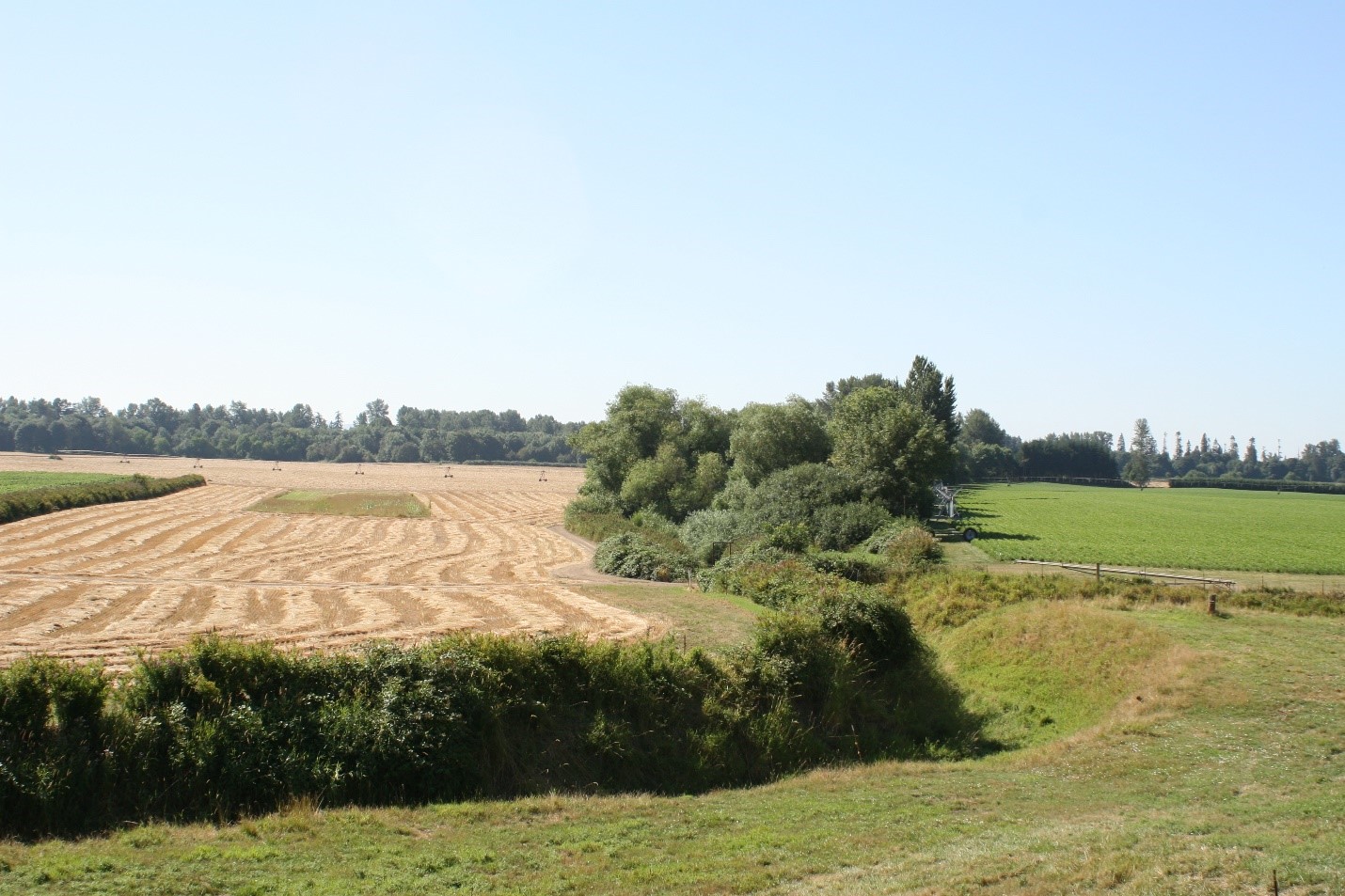
Chapter Summary
Agroecosystems
Agriculture provides immense social benefit, but it also threatens our well-being through its effects on the Earth System. We are beginning to explore ways to reconcile that conundrum by designing more sustainable and ecologically integrated farming systems.
- We can describe farming systems in ecological terms (Figures 7.3, 7.4) and assess their ecological impact using tools such as life cycle assessment (Figures 7.5, 7.6) and efficiency metrics (Table 7.2, Figures 7.7, 7.8, 7.9)
- Agriculture is a significant force pushing the Earth System past planetary boundaries (Figure 7.11)
- The conversion of carbon dense landscapes into agriculture, as well as ongoing farming practices are significant sources of greenhouse gas emissions (Figure 7.12).
- Agroecosystems are significant sources of nutrient pollution because they are dominated by crops that are poor at nutrient capture (Figure 7.13), they have low levels of resource complementarity, their trophic structure is spatially disarticulated (Figure 7.14), and they have high rates of soil erosion (Figure 7.15). In addition, we imprecisely add nutrients at times, places, and in forms that foster leakage.
- Agriculture appropriates 92% of the water humanity uses. In some regions that use is a significant contributor to water scarcity (Figures 7.16, 7.17).
- The conversion of biodiverse landscapes into less diverse agricultural landscapes (Figure 7.18) as well as the intensification of farming practices (Figure 7.21) are significant drivers of biodiversity loss.
- Improve the resource use efficiency of farming can lessen its ecological impact. Strategies include creating more resource capture efficient crops, applying resources more precisely (Figure 7.24), reducing tillage (Figure 7.26), and adopting integrated pest management.
- We can improve the efficiency of the broader food system by reducing waste along the food supply chain, reducing animal production (Figures 7.27, 7.28), and reducing the knowledge and resource gaps experienced by many farmers.
- Enhancing the ecological functioning of agroecosystems can also mitigate its ecological impact. Techniques include various forms of spatial polyculture (Figures 7.29, 7.30), diverse crop rotations (Figure 7.31), and integrating crop and livestock production (Figure 7.32).
- We can also foster the ability of natural enemies to regulate crop pests. A main approach is to create and maintain habitat for natural enemies (Figure 7.33, 7.34).
- We can include biodiversity conservation as an explicit design goal for our agroecosystems. Techniques include restoring portions of agricultural landscapes into biodiversity supporting habitat and managing farmed landscapes in ways that enhance their habitat value (Figure 7.35).
Additional Resources
- The King of California: J. G. Boswell and the Making of a Secret American Empire, by Mark Arax and Rick Wartzman (New York: PublicAffairs, 2003). This book tells the specific story of the Boswells, who became the largest family farmers in the United States, as well as the broader story of how agro-industrialization transformed the Central Valley of California
- The King of California: J. G. Boswell and the Making of a Secret American Empire, by Mark Arax and Rick Wartzman (New York: PublicAffairs, 2003). This book tells the specific story of the Boswells, who became the largest family farmers in the United States, as well as the broader story of how agro-industrialization transformed the Central Valley of California
- Tending the Wild: Native American Knowledge and the Management of California’s Natural Resources, by M. Kat Anderson (Berkeley: University of California Press, 2005). An exploration of how Indigenous peoples used and shaped California’s natural resources
- This series of presentations by the US Department of Agriculture Natural Resources Conservation Service takes you on a road trip across the country to see various ways that farmers are implementing conservation and integrating ecological processes into their farming systems: Cascade NRCS
- In this video, chef Dan Barber talks about his search for a sustainable fish to serve on his menu. He finds it at Veta La Palma, an innovative aquaculture operation in Spain: How I Fell in Love with a Fish
References
113Abioye, E.A., Abidin, M.S.Z., Mahmud, M.S.A., Buyamin, S., Ishak, M.H.I., Rahman, M.K.I.A., Otuoze, A.O., Onotu, P., Ramli, M.S.A., 2020. A review on monitoring and advanced control strategies for precision irrigation. Comput. Electron. Agric. 173, 105441. https://doi.org/10.1016/j.compag.2020.105441
52*Alewell, C., Ringeval, B., Ballabio, C., Robinson, D.A., Panagos, P., Borrelli, P., 2020. Global phosphorus shortage will be aggravated by soil erosion. Nat. Commun. 11, 4546. https://doi.org/10.1038/s41467-020-18326-7
120* Alexander, P., Brown, C., Arneth, A., Finnigan, J., Moran, D., Rounsevell, M.D.A., 2017. Losses, inefficiencies and waste in the global food system. Agric. Syst. 153, 190–200. https://doi.org/10.1016/j.agsy.2017.01.014
*Ali, M. P., Bari, M. N., Haque, S. S., Kabir, M. M. M., Afrin, S., Nowrin, F., Islam, M. S., & Landis, D. A. (2019). Establishing next-generation pest control services in rice fields: Eco-agriculture. Scientific Reports, 9(1), Article 1. https://doi.org/10.1038/s41598-019-46688-6
3Anderson, K., 2005. Tending the Wild: Native American Knowledge and the Management of California’s Natural Resources. Berkeley: University of California Press.
9Arax, M., 2018. A kingdom from dust. California Sunday Magazine, January 31, 2018.
6712Arax, M., Wartzman, R., 2003. The King of California: J. G. Boswell and the Making of a Secret American Empire. New York: PublicAffairs.
19Baker, P., 2014. Global coffee production and land use change. Presented at the 25th Conference of ASIC (Association Scientifique Internationale pour le Café), Calarcá, Colombia.
7879Batáry, P., Gallé, R., Riesch, F., Fischer, C., Dormann, C.F., Mußhoff, O., Császár, P., Fusaro, S., Gayer, C., Happe, A.-K., Kurucz, K., Molnár, D., Rösch, V., Wietzke, A., Tscharntke, T., 2017. The former Iron Curtain still drives biodiversity–profit trade-offs in German agriculture. Nat. Ecol. Evol. 1, 1279–84. https://doi.org/10.1038/s41559-017-0272-x
74Benton, T.G., Vickery, J.A., Wilson, J.D., 2003. Farmland biodiversity: is habitat heterogeneity the key? Trends Ecol. Evol. 18, 182–88. https://doi.org/10.1016/S0169-5347(03)00011-9
22Bogaard, A., Fochesato, M., Bowles, S., 2019. The farming-inequality nexus: new insights from ancient western Eurasia. Antiquity 93, 1129–1143. https://doi.org/10.15184/aqy.2019.105
116Borel, B., 2017. When the pesticides run out. Nature 543, 302–4.
51Borrelli, P., Robinson, D.A., Panagos, P., Lugato, E., Yang, J.E., Alewell, C., Wuepper, D., Montanarella, L., Ballabio, C., 2020. Land use and climate change impacts on global soil erosion by water (2015-2070). Proc. Natl. Acad. Sci. 117, 21,994–22,001. https://doi.org/10.1073/pnas.2001403117
141*Bowles, T.M., Mooshammer, M., Socolar, Y., Calderón, F., Cavigelli, M.A., Culman, S.W., Deen, W., Drury, C.F., Garcia y Garcia, A., Gaudin, A.C.M., Harkcom, W.S., Lehman, R.M., Osborne, S.L., Robertson, G.P., Salerno, J., Schmer, M.R., Strock, J., Grandy, A.S., 2020. Long-term evidence shows that crop-rotation diversification increases agricultural resilience to adverse growing conditions in North America. One Earth 2, 284–93. https://doi.org/10.1016/j.oneear.2020.02.007
85Brühl, C.A., Bakanov, N., Köthe, S., Eichler, L., Sorg, M., Hörren, T., Mühlethaler, R., Meinel, G., Lehmann, G.U.C., 2021. Direct pesticide exposure of insects in nature conservation areas in Germany. Sci. Rep. 11, 24144. https://doi.org/10.1038/s41598-021-03366-w
149Buck, B.H., Troell, M.F., Krause, G., Angel, D.L., Grote, B., Chopin, T., 2018. State of the art and challenges for offshore integrated multi-trophic aquaculture (IMTA). Front. Mar. Sci. 5. https://doi.org/10.3389/fmars.2018.00165
96Cabodevilla, X., Wright, A.D., Villanua, D., Arroyo, B., Zipkin, E.F., 2022. The implementation of irrigation leads to declines in farmland birds. Agric. Ecosyst. Environ. 323, 107701. https://doi.org/10.1016/j.agee.2021.107701
2California Department of Food and Agriculture, 2020. California Agricultural Statistics Review, 2019-2020. Sacramento: California Department of Food and Agriculture.
*576064Campbell, B., Beare, D., Bennett, E., Hall-Spencer, J., Ingram, J., Jaramillo, F., Ortiz, R., Ramankutty, N., Sayer, J., Shindell, D., 2017. Agriculture production as a major driver of the Earth System exceeding planetary boundaries. Ecol. Soc. 22. https://doi.org/10.5751/ES-09595-220408
*Campos, J., Gallart, M., Llop, J., Ortega, P., Salcedo, R., Gil, E., 2020. On-farm evaluation of prescription map-based variable rate application of pesticides in vineyards. Agronomy 10, 102. https://doi.org/10.3390/agronomy10010102
41Carpenter, S.R., Bennett, E.M., 2011. Reconsideration of the planetary boundary for phosphorus. Environ. Res. Lett. 6, 014009. https://doi.org/10.1088/1748-9326/6/1/014009
119Carson, R., 1962. Silent Spring. Cambridge, MA: Houghton Mifflin.
l26127Cassidy, E.S., West, P.C., Gerber, J.S., Foley, J.A., 2013. Redefining agricultural yields: from tonnes to people nourished per hectare. Environ. Res. Lett. 8, 034015. https://doi.org/10.1088/1748-9326/8/3/034015
45Christianson, L.E., Harmel, R.D., 2015. 4R water quality impacts: an assessment and synthesis of forty years of drainage nitrogen losses. J. Environ. Qual. 44, 1852–60. https://doi.org/10.2134/jeq2015.03.0170
142Clark, I., Jones, S.S., Reganold, J.P., Sanguinet, K.A., Murphy, K.M., 2019. Agronomic performance of perennial grain genotypes in the Palouse region of the Pacific Northwest, USA. Front. Sustainable Food Syst. 3.
141Clark, M.S., Gage, S.H., 1996. Effects of free-range chickens and geese on insect pests and weeds in an agroecosystem. Am. J. Altern. Agric. 11, 39–47. https://doi.org/10.1017/S0889189300006718
27Congreves, K.A., Otchere, O., Ferland, D., Farzadfar, S., Williams, S., Arcand, M.M., 2021. Nitrogen use efficiency definitions of today and tomorrow. Front. Plant Sci. 12, 637108. doi:10.3389/fpls.2021.637108.
170Cotterman, K.A., Kendall, A.D., Basso, B., Hyndman, D.W., 2018. Groundwater depletion and climate change: future prospects of crop production in the Central High Plains Aquifer. Clim. Change 146, 187–200. https://doi.org/10.1007/s10584-017-1947-7
35Covey, K., Soper, F., Pangala, S., Bernardino, A., Pagliaro, Z., Basso, L., Cassol, H., Fearnside, P., Navarrete, D., Novoa, S., Sawakuchi, H., Lovejoy, T., Marengo, J., Peres, C.A., Baillie, J., Bernasconi, P., Camargo, J., Freitas, C., Hoffman, B., Nardoto, G.B., Nobre, I., Mayorga, J., Mesquita, R., Pavan, S., Pinto, F., Rocha, F., de Assis Mello, R., Thuault, A., Bahl, A.A., Elmore, A., 2021. Carbon and beyond: the biogeochemistry of climate in a rapidly changing Amazon. Front. For. Global Change 4. https://doi.org/10.3389/ffgc.2021.618401
75Crossley, M.S., Burke, K.D., Schoville, S.D., Radeloff, V.C., 2021. Recent collapse of crop belts and declining diversity of US agriculture since 1840. Global Change Biol. 27, 151–64. https://doi.org/10.1111/gcb.15396
31Crowther, T.W., Glick, H.B., Covey, K.R., Bettigole, C., Maynard, D.S., Thomas, S.M., Smith, J.R., Hintler, G., Duguid, M.C., Amatulli, G., Tuanmu, M.-N., Jetz, W., Salas, C., Stam, C., Piotto, D., Tavani, R., Green, S., Bruce, G., Williams, S.J., Wiser, S.K., Huber, M.O., Hengeveld, G.M., Nabuurs, G.-J., Tikhonova, E., Borchardt, P., Li, C.-F., Powrie, L.W., Fischer, M., Hemp, A., Homeier, J., Cho, P., Vibrans, A.C., Umunay, P.M., Piao, S.L., Rowe, C.W., Ashton, M.S., Crane, P.R., Bradford, M.A., 2015. Mapping tree density at a global scale. Nature 525, 201–5. https://doi.org/10.1038/nature14967
103Dai, J., Bean, B., Brown, B., Bruening, W., Edwards, J., Flowers, M., Karow, R., Lee, C., Morgan, G., Ottman, M., Ransom, J., Wiersma, J., 2016. Harvest index and straw yield of five classes of wheat. Biomass Bioenergy 85, 223–27. https://doi.org/10.1016/j.biombioe.2015.12.023
159Dainese, M., Montecchiari, S., Sitzia, T., Sigura, M., Marini, L., 2016. High cover of hedgerows in the landscape supports multiple ecosystem services in Mediterranean cereal fields. J. Appl. Ecol. 54, 380–88. https://doi.org/10.1111/1365-2664.12747
*de Faccio Carvalho, P.C., de Albuquerque Nunes, P.A., Pontes-Prates, A., Szymczak, L.S., de Souza Filho, W., Moojen, F.G., Lemaire, G., 2021. Reconnecting grazing livestock to crop landscapes: reversing specialization trends to restore landscape multifunctionality. Front. Sustainable Food Syst. 5. https://doi.org/10.3389/fsufs.2021.750765
90de Graaff, M.-A., Hornslein, N., Throop, H.L., Kardol, P., van Diepen, L.T.A., 2019. Effects of agricultural intensification on soil biodiversity and implications for ecosystem functioning: a meta-analysis. In: Sparks, D.L. (Ed.), Advances in Agronomy. San Diego, CA: Academic Press, 1–44. https://doi.org/10.1016/bs.agron.2019.01.001
102Denison, R.F., 2012. Darwinian Agriculture: How Understanding Evolution Can Improve Agriculture. Princeton, NJ: Princeton University Press.
83DiBartolomeis, M., Kegley, S., Mineau, P., Radford, R., Klein, K., 2019. An assessment of acute insecticide toxicity loading (AITL) of chemical pesticides used on agricultural land in the United States. PLoS One 14, e0220029. https://doi.org/10.1371/journal.pone.0220029
125Dijkink, B., Broeze, J., Vollebregt, M., 2022. Hermetic bags for the storage of maize: perspectives on economics, food security and greenhouse gas emissions in different sub-Saharan African countries. Front. Sustainable Food Syst. 6.
13Dobermann, D., Swift, J.A., Field, L.M., 2017. Opportunities and hurdles of edible insects for food and feed. Nutr. Bull. 42, 293–308. https://doi.org/10.1111/nbu.12291
73Dondina, O., Saura, S., Bani, L., Mateo-Sánchez, M.C., 2018. Enhancing connectivity in agroecosystems: focus on the best existing corridors or on new pathways? Landscape Ecol. 33, 1741–56. https://doi.org/10.1007/s10980-018-0698-9
171Donlan, C.J., Berger, J., Bock, C.E., Bock, J.H., Burney, D.A., Estes, J.A., Foreman, D., Martin, P.S., Roemer, G.W., Smith, F.A., Soulé, M.E., Greene, H.W., 2015. Pleistocene rewilding: an optimistic agenda for twenty‐first century conservation. Am. Nat. 168. https://doi.org/10.1086/508027
89Dorrough, J., Scroggie, M.P., 2008. Plant responses to agricultural intensification. J. Appl. Ecol. 45, 1274–83. https://doi.org/10.1111/j.1365-2664.2008.01501.x
*Duiker, S.W., Myers, J.C., Blazure, L.C., 2017. Soil Health in Field and Forage Crop Production. US Department of Agriculture, Natural Resources Conservation Service; Harrisburg, PA: Penn State Cooperative Extension,.
144Edwards, J.T., Carver, B.F., Horn, G.W., Payton, M.E., 2011. Impact of dual-purpose management on wheat grain yield. Crop Sci. 51, 2181–85. https://doi.org/10.2135/cropsci2011.01.0043
129Ehleringer, J.R., Covarrubias Avalos, S., Tipple, B.J., Valenzuela, L.O., Cerling, T.E., 2020. Stable isotopes in hair reveal dietary protein sources with links to socioeconomic status and health. Proc. Natl. Acad. Sci. 117, 20,044–51. https://doi.org/10.1073/pnas.1914087117
95Eng, M.L., Stutchbury, B.J.M., Morrissey, C.A., 2019. A neonicotinoid insecticide reduces fueling and delays migration in songbirds. Science 365, 1177-80. https://doi.org/10.1126/science.aaw9419
33Erb, K.-H., Kastner, T., Plutzar, C., Bais, A.L.S., Carvalhais, N., Fetzel, T., Gingrich, S., Haberl, H., Lauk, C., Niedertscheider, M., Pongratz, J., Thurner, M., Luyssaert, S., 2018. Unexpectedly large impact of forest management and grazing on global vegetation biomass. Nature 553, 73–76. https://doi.org/10.1038/nature25138
148Estim, A., 2015. Integrated multitrophic aquaculture. In: Aquaculture Ecosystems. Hoboken, NJ: Wiley-Blackwell, 164–81. https://doi.org/10.1002/9781118778531.ch6
136Exner, D.N., Davidson, D.G., Ghaffarzadeh, M., Cruse, R.M., 1999. Yields and returns from strip intercropping on six Iowa farms. Am. J. Altern. Agric. 14, 69–77. https://doi.org/10.1017/S0889189300008092
111Field, K.J., Daniell, T., Johnson, D., Helgason, T., 2020. Mycorrhizas for a changing world: sustainability, conservation, and society. Plants People Planet 2, 98–103. https://doi.org/10.1002/ppp3.10092
20Filho, W.L., Barbir, J., Preziosi, R., 2018. Handbook of Climate Change and Biodiversity. New York: Springer.
121Foley, J.A., Ramankutty, N., Brauman, K.A., Cassidy, E.S., Gerber, J.S., Johnston, M., Mueller, N.D., O’Connell, C., Ray, D.K., West, P.C., Balzer, C., Bennett, E.M., Carpenter, S.R., Hill, J., Monfreda, C., Polasky, S., Rockström, J., Sheehan, J., Siebert, S., Tilman, D., Zaks, D.P.M., 2011. Solutions for a cultivated planet. Nature 478, 337–42. https://doi.org/10.1038/nature10452
*Friedli, C.N., Abiven, S., Fossati, D., Hund, A., 2019. Modern wheat semi-dwarfs root deep on demand: response of rooting depth to drought in a set of Swiss era wheats covering 100 years of breeding. Euphytica 215, 85. https://doi.org/10.1007/s10681-019-2404-7
46Furey, G.N., Tilman, D., 2021. Plant biodiversity and the regeneration of soil fertility. Proc. Natl. Acad. Sci. 118. https://doi.org/10.1073/pnas.2111321118
40Galloway, J.N., Townsend, A.R., Erisman, J.W., Bekunda, M., Cai, Z., Freney, J.R., Martinelli, L.A., Seitzinger, S.P., Sutton, M.A., 2008. Transformation of the nitrogen cycle: recent trends, questions, and potential solutions. Science 320, 889–92. https://doi.org/10.1126/science.1136674
14Gannon, M., 2017. A new Antarctic-proof greenhouse heads south to polar scientists. Scientific American, February 1, 2017. https://doi.org/10.1038/scientificamerican0217-18a
34Gasser, T., Crepin, L., Quilcaille, Y., Houghton, R.A., Ciais, P., Obersteiner, M., 2020. Historical CO2 emissions from land use and land cover change and their uncertainty. Biogeosciences 17, 4075–101. https://doi.org/10.5194/bg-17-4075-2020
93Geffroy, L., 2018. Where have all the farmland birds gone? CNRS News, March 21, 2018. https://news.cnrs.fr/articles/where-have-all-the-farmland-birds-gone.
140Gentry, L.F., Ruffo, M.L., Below, F.E., 2013. Identifying factors controlling the continuous corn yield penalty. Agron. J. 105, 295–303. https://doi.org/10.2134/agronj2012.0246
66Gibbs, H.K., Ruesch, A.S., Achard, F., Clayton, M.K., Holmgren, P., Ramankutty, N., Foley, J.A., 2010. Tropical forests were the primary sources of new agricultural land in the 1980s and 1990s. Proc. Natl. Acad. Sci. 107, 16,732–37. https://doi.org/10.1073/pnas.0910275107
114Giles, D., Klassed, P., Niederholzer, F., Downey, D., 2011. “Smart” sprayer technology provides environmental and economic benefits in California orchards. Calif. Agric. 65, 85–89.
84Goulson, D., Thompson, J., Croombs, A., 2018. Rapid rise in toxic load for bees revealed by analysis of pesticide use in Great Britain. PeerJ 6, e5255. https://doi.org/10.7717/peerj.5255
*Gray, E., 2012. Landsat top ten—a shrinking sea, Aral Sea. NASA, July 23, 2012. https://www.nasa.gov/mission_pages/landsat/news/40th-top10-aralsea.html.
169Haacker, E.M.K., Kendall, A.D., Hyndman, D.W., 2016. Water level declines in the high plains aquifer: predevelopment to resource senescence. Groundwater 54, 231–42. https://doi.org/10.1111/gwat.12350
48Hacker, N., Ebeling, A., Gessler, A., Gleixner, G., González Macé, O., de Kroon, H., Lange, M., Mommer, L., Eisenhauer, N., Ravenek, J., Scheu, S., Weigelt, A., Wagg, C., Wilcke, W., Oelmann, Y., 2015. Plant diversity shapes microbe-rhizosphere effects on P mobilisation from organic matter in soil. Ecol. Lett. 18, 1356–65. https://doi.org/10.1111/ele.12530
166Haddaway, N.R., Brown, C., Eggers, S., Josefsson, J., Kronvang, B., Randall, N., Uusi-Kämppä, J., 2016. The multifunctional roles of vegetated strips around and within agricultural fields: a systematic map protocol. Environ. Evidence 5, 18. https://doi.org/10.1186/s13750-016-0067-6
49Hamlin, Q.F., Kendall, A.D., Martin, S.L., Whitenack, H.D., Roush, J.A., Hannah, B.A., Hyndman, D.W., 2020. Quantifying landscape nutrient inputs with spatially explicit nutrient source estimate maps. J. Geophys. Res. Biogeosci. 125, e2019JG005134. https://doi.org/10.1029/2019JG005134
88Han, P., Lavoir, A.-V., Rodriguez-Saona, C., Desneux, N., 2022. Bottom-up forces in agroecosystems and their potential impact on arthropod pest management. Annu. Rev. Entomol. 67, 239–59. https://doi.org/10.1146/annurev-ento-060121-060505
72163165Heath, S.K., Soykan, C.U., Velas, K.L., Kelsey, R., Kross, S.M., 2017. A bustle in the hedgerow: woody field margins boost on farm avian diversity and abundance in an intensive agricultural landscape. Biol. Conserv. 212, 153–61. https://doi.org/10.1016/j.biocon.2017.05.031
174Hegyi, N., 2019. Big money is building a new kind of national park in the Great Plains. NPR, December 8, 2019.
77Hemberger, J., Crossley, M.S., Gratton, C., 2021. Historical decrease in agricultural landscape diversity is associated with shifts in bumble bee species occurrence. Ecol. Lett. 24, 1800–1813. https://doi.org/10.1111/ele.13786
11Herrero, M., Thornton, P.K., Power, B., Bogard, J.R., Remans, R., Fritz, S., Gerber, J.S., Nelson, G., See, L., Waha, K., Watson, R.A., West, P.C., Samberg, L.H., van de Steeg, J., Stephenson, E., van Wijk, M., Havlík, P., 2017. Farming and the geography of nutrient production for human use: a transdisciplinary analysis. Lancet Planet. Health 1, e33–e42. https://doi.org/10.1016/S2542-5196(17)30007-4
545556*59Hoekstra, A.Y., Mekonnen, M.M., 2012. The water footprint of humanity. Proc. Natl. Acad. Sci. 109, 3232–37. https://doi.org/10.1073/pnas.1109936109
105Horton, P., Long, S.P., Smith, P., Banwart, S.A., Beerling, D.J., 2021. Technologies to deliver food and climate security through agriculture. Nat. Plants 7, 250–55. https://doi.org/10.1038/s41477-021-00877-2
146Hu, L., Zhang, Jian, Ren, W., Guo, L., Cheng, Y., Li, J., Li, K., Zhu, Z., Zhang, Jiaen, Luo, S., Cheng, L., Tang, J., Chen, X., 2016. Can the co-cultivation of rice and fish help sustain rice production? Sci. Rep. 6, 28728. https://doi.org/10.1038/srep28728
157Iuliano, B., Gratton, C., 2020. Temporal resource (dis)continuity for conservation biological control: from field to landscape scales. Front. Sustainable Food Syst. 4.
122Jaglo, K., Kenny, S., Stephenson, J., 2021. From Farm to Kitchen: The Environmental Impacts of U.S. Food Waste. No. EPA 600-R21 171. Washington, DC: US Environmental Protection Agency.
*Joint Nature Conservation Committee, 2021. UK Biodiversity Indicators 2021. London: Department for Environment, Food and Rural Affairs.
91Kehoe, L., Romero-Muñoz, A., Polaina, E., Estes, L., Kreft, H., Kuemmerle, T., 2017. Biodiversity at risk under future cropland expansion and intensification. Nat. Ecol. Evol. 1, 1129–35. https://doi.org/10.1038/s41559-017-0234-3
124Kibiti, B., Strubenhoff, B.K., 2019. How off-grid cold storage systems can help farmers reduce post-harvest losses. Brookings, October 16, 2019. https://www.brookings.edu/blog/future-development/2019/10/16/how-off-grid-cold-storage-systems-can-help-farmers-reduce-post-harvest-losses/.
175Kim, T.N., Fox, A.F., Wills, B.D., Meehan, T.D., Landis, D.A., Gratton, C., 2017. Harvesting biofuel grasslands has mixed effects on natural enemy communities and no effects on biocontrol services. J. Appl. Ecol. 54, 2011–21. https://doi.org/10.1111/1365-2664.12901
32Knox, S.H., Sturtevant, C., Matthes, J.H., Koteen, L., Verfaillie, J., Baldocchi, D., 2015. Agricultural peatland restoration: effects of land-use change on greenhouse gas (CO2 and CH4) fluxes in the Sacramento-San Joaquin Delta. Global Change Biol. 21, 750–65. https://doi.org/10.1111/gcb.12745
158 Kremen, C., 2020. Ecological intensification and diversification approaches to maintain biodiversity, ecosystem services and food production in a changing world. Emerging Top. Life Sci. 4, 229–40. https://doi.org/10.1042/ETLS20190205
164 Kremen, C., M’Gonigle, L.K., 2015. Small-scale restoration in intensive agricultural landscapes supports more specialized and less mobile pollinator species. J. Appl. Ecol. 52, 602–10. https://doi.org/10.1111/1365-2664.12418
16Kroeger, A., Bakhtary, H., Haupt, F., Streck, C., 2017. Eliminating Deforestation from the Cocoa Supply Chain (working paper). Washington, DC: World Bank. https://doi.org/10.1596/26549
153Kross, S.M., Martinico, B.L., Bourbour, R.P., Townsend, J.M., McColl, C., Kelsey, T.R., 2020. Effects of field and landscape scale habitat on insect and bird damage to sunflowers. Front. Sustainable Food Syst. 4.
*284247Lassaletta, L., Billen, G., Grizzetti, B., Anglade, J., Garnier, J., 2014. 50 year trends in nitrogen use efficiency of world cropping systems: the relationship between yield and nitrogen input to cropland. Environ. Res. Lett. 9, 105011. https://doi.org/10.1088/1748-9326/9/10/105011
154Lee-Mäder, E., Society, X., 2014. Farming with Native Beneficial Insects: Ecological Pest Control Solutions. North Adams, MA: Storey Publishing.
10Lesiv, M., Laso Bayas, J.C., See, L., Duerauer, M., Dahlia, D., Durando, N., Hazarika, R., Kumar Sahariah, P., Vakolyuk, M., Blyshchyk, V., Bilous, A., Perez-Hoyos, A., Gengler, S., Prestele, R., Bilous, S., Akhtar, ul Hassan Akhtar, I., Singha, K., Choudhury, S.B., Chetri, T., Malek, Ž., Bungnamei, K., Saikia, A., Sahariah, D., Narzary, W., Danylo, O., Sturn, T., Karner, M., McCallum, I., Schepaschenko, D., Moltchanova, E., Fraisl, D., Moorthy, I., Fritz, S., 2019. Estimating the global distribution of field size using crowdsourcing. Global Change Biol. 25, 174–86. https://doi.org/10.1111/gcb.14492
25Lollato, R.P., Edwards, J.T., Ochsner, T.E., 2017. Meteorological limits to winter wheat productivity in the U.S. southern Great Plains. Field Crops Res. 203, 212–26. https://doi.org/10.1016/j.fcr.2016.12.014
101López-Calcagno, P.E., Brown, K.L., Simkin, A.J., Fisk, S.J., Vialet-Chabrand, S., Lawson, T., Raines, C.A., 2020. Stimulating photosynthetic processes increases productivity and water-use efficiency in the field. Nat. Plants 6, 1054–63. https://doi.org/10.1038/s41477-020-0740-1
134*Lopez-Ridaura, S., Barba-Escoto, L., Reyna-Ramirez, C.A., Sum, C., Palacios-Rojas, N., Gerard, B., 2021. Maize intercropping in the milpa system: diversity, extent and importance for nutritional security in the Western Highlands of Guatemala. Sci. Rep. 11, 3696. https://doi.org/10.1038/s41598-021-82784-2
4344Lun, F., Liu, J., Ciais, P., Nesme, T., Chang, J., Wang, R., Goll, D., Sardans, J., Peñuelas, J., Obersteiner, M., 2018. Global and regional phosphorus budgets in agricultural systems and their implications for phosphorus-use efficiency. Earth Syst. Sci. Data 10, 1–18. https://doi.org/10.5194/essd-10-1-2018
62Mekonnen, M.M., Hoekstra, A.Y., 2016. Four billion people facing severe water scarcity. Sci. Adv. 2, e1500323. https://doi.org/10.1126/sciadv.1500323
69Meyer, S., Wesche, K., Krause, B., Leuschner, C., 2013. Dramatic losses of specialist arable plants in central Germany since the 1950s/60s—a cross-regional analysis. Diversity Distrib. 19, 1175–87. https://doi.org/10.1111/ddi.12102
143Michaels, J., Batzer, E., Harrison, S., Eviner, V.T., 2021. Grazing affects vegetation diversity and heterogeneity in California vernal pools. Ecology 102, e03295. https://doi.org/10.1002/ecy.3295
61Micklin, P., 2007. The Aral Sea disaster. Annu. Rev. Earth Planet. Sci. 35, 47–72. https://doi.org/10.1146/annurev.earth.35.031306.140120
94Møller, A.P., Czeszczewik, D., Flensted-Jensen, E., Erritzøe, J., Krams, I., Laursen, K., Liang, W., Walankiewicz, W., 2021. Abundance of insects and aerial insectivorous birds in relation to pesticide and fertilizer use. Avian Res. 12, 43. https://doi.org/10.1186/s40657-021-00278-1
155Morandin, L., Long, R., Pease, C., Kremen, C., 2011. Hedgerows enhance beneficial insects on farms in California’s Central Valley. Calif. Agric. 65, 197–201.
118Móring, A., Hooda, S., Raghuram, N., Adhya, T.K., Ahmad, A., Bandyopadhyay, S.K., Barsby, T., Beig, G., Bentley, A.R., Bhatia, A., Dragosits, U., Drewer, J., Foulkes, J., Ghude, S.D., Gupta, R., Jain, N., Kumar, D., Kumar, R.M., Ladha, J.K., Mandal, P.K., Neeraja, C.N., Pandey, R., Pathak, H., Pawar, P., Pellny, T.K., Poole, P., Price, A., Rao, D.L.N., Reay, D.S., Singh, N.K., Sinha, S.K., Srivastava, R.K., Shewry, P., Smith, J., Steadman, C.E., Subrahmanyam, D., Surekha, K., Venkatesh, K., Varinderpal-Singh, Uwizeye, A., Vieno, M., Sutton, M.A., 2021. Nitrogen challenges and opportunities for agricultural and environmental science in India. Front. Sustainable Food Syst. 5.
24Mueller, N.D., Gerber, J.S., Johnston, M., Ray, D.K., Ramankutty, N., Foley, J.A., 2012. Closing yield gaps through nutrient and water management. Nature 490, 254–57. https://doi.org/10.1038/nature11420
5Muir, J., 1894. The Mountains of California. Century Company.
130Nardoto, G.B., Sena-Souza, J.P., Kisaka, T.B., Costa, F.J.V., Duarte-Neto, P.J., Ehleringer, J., Martinelli, L.A., 2020. Increased in carbon isotope ratios of Brazilian fingernails are correlated with increased in socioeconomic status. Npj Sci. Food 4, 9. https://doi.org/10.1038/s41538-020-0069-1
63Newbold, T., Hudson, L.N., Hill, S.L.L., Contu, S., Lysenko, I., Senior, R.A., Börger, L., Bennett, D.J., Choimes, A., Collen, B., Day, J., Palma, A.D., Díaz, S., Echeverria-Londoño, S., Edgar, M.J., Feldman, A., Garon, M., Harrison, M.L.K., Alhusseini, T., Ingram, D.J., Itescu, Y., Kattge, J., Kemp, V., Kirkpatrick, L., Kleyer, M., Correia, D.L.P., Martin, C.D., Meiri, S., Novosolov, M., Pan, Y., Phillips, H.R.P., Purves, D.W., Robinson, A., Simpson, J., Tuck, S.L., Weiher, E., White, H.J., Ewers, R.M., Mace, G.M., Scharlemann, J.P.W., Purvis, A., 2015. Global effects of land use on local terrestrial biodiversity. Nature 520, 45–50. https://doi.org/10.1038/nature14324
17Niether, W., Jacobi, J., Blaser, W.J., Andres, C., Armengot, L., 2020. Cocoa agroforestry systems versus monocultures: a multi-dimensional meta-analysis. Environ. Res. Lett. 15, 104085. https://doi.org/10.1088/1748-9326/abb053
*NRCS. Natural Resources Conservation Service, 2005. Conservation Practices that Save: Nutrient Management. Athens: NRCS Georgia.
150Oerke, E.-C., 2006. Crop losses to pests. J. Agric. Sci. 144, 31–43. https://doi.org/10.1017/S0021859605005708
*Orozco-Aguilar, L., López-Sampson, A., Leandro-Muñoz, M.E., Robiglio, V., Reyes, M., Bordeaux, M., Sepúlveda, N., Somarriba, E., 2021. Elucidating pathways and discourses linking cocoa cultivation to deforestation, reforestation, and tree cover change in Nicaragua and Peru. Front. Sustainable Food Syst. 5, 199. https://doi.org/10.3389/fsufs.2021.635779
147Palm, H.W., Knaus, U., Appelbaum, S., Goddek, S., Strauch, S.M., Vermeulen, T., Haїssam Jijakli, M., Kotzen, B., 2018. Towards commercial aquaponics: a review of systems, designs, scales and nomenclature. Aquacult. Int. 26, 813–42. https://doi.org/10.1007/s10499-018-0249-z
23Phalan, B., Green, R., Balmford, A., 2014. Closing yield gaps: perils and possibilities for biodiversity conservation. Philos. Trans. R. Soc. B Biol. Sci. 369, 20120285. https://doi.org/10.1098/rstb.2012.0285
38**Poore, J., Nemecek, T., 2018. Reducing food’s environmental impacts through producers and consumers. Science 360, 987-92. https://doi.org/10.1126/science.aaq0216
160Prasad, R.P., Snyder, W.E., 2006. Polyphagy complicates conservation biological control that targets generalist predators. J. Appl. Ecol. 43, 343–52. https://doi.org/10.1111/j.1365-2664.2006.01129.x
151Précigout, P.-A., Robert, C., 2022. Effects of hedgerows on the preservation of spontaneous biodiversity and the promotion of biotic regulation services in agriculture: towards a more constructive relationships between agriculture and biodiversity. Bot. Lett. 0, 1–29. https://doi.org/10.1080/23818107.2022.2053205
50Quinton, J.N., Govers, G., Oost, K.V., Bardgett, R.D., 2010. The impact of agricultural soil erosion on biogeochemical cycling. Nat. Geosci. 3, 311–14. https://doi.org/10.1038/ngeo838
128Ramankutty, N., Mehrabi, Z., Waha, K., Jarvis, L., Kremen, C., Herrero, M., Rieseberg, L.H., 2018. Trends in global agricultural land use: implications for environmental health and food security. Annu. Rev. Plant Biol. 69, 789–815. https://doi.org/10.1146/annurev-arplant-042817-040256
138Reiss, E.R., Drinkwater, L.E., 2018. Cultivar mixtures: a meta-analysis of the effect of intraspecific diversity on crop yield. Ecol. Appl. 28, 62–77. https://doi.org/10.1002/eap.1629
58Richter, B., 2014. How to survive a water crisis: Murray-Darling Basin, Australia. In: Richter, B. (Ed.), Chasing Water: A Guide for Moving from Scarcity to Sustainability. Washington, DC: Island Press/Center for Resource Economics, 117–40. https://doi.org/10.5822/978-1-61091-537-3_7
108Rillig, M.C., Aguilar-Trigueros, C.A., Camenzind, T., Cavagnaro, T.R., Degrune, F., Hohmann, P., Lammel, D.R., Mansour, I., Roy, J., van der Heijden, M.G.A., Yang, G., 2019. Why farmers should manage the arbuscular mycorrhizal symbiosis. New Phytol. 222, 1171–75. https://doi.org/10.1111/nph.15602
*Ritchie, H., 2019. Food production is responsible for one-quarter of the world’s greenhouse gas emissions. Our World Data, November 6, 2019. https://ourworldindata.org/food-ghg-emissions.
*Ritchie, H., 2021. Can we reduce fertilizer use without sacrificing food production? Our World Data, September 9, 2021. https://ourworldindata.org/reducing-fertilizer-use.
*Ritchie, H., Roser, M., 2019. Meat and dairy production. Our World Data. Last revised June 2019, https://ourworldindata.org/meat-production.
*Ritchie, H., Roser, M., 2021. Environmental impacts of food production. Our World Data. Last revised June 2021, https://ourworldindata.org/environmental-impacts-of-food.
152Russell, M.C., Lambrinos, J., Records, E., Ellen, G., 2017. Seasonal shifts in ground beetle (Coleoptera: Carabidae) species and functional composition maintain prey consumption in western Oregon agricultural landscapes. Biol. Control 106, 54–63. https://doi.org/10.1016/j.biocontrol.2016.12.008
110Ryan, M.H., Graham, J.H., 2018. Little evidence that farmers should consider abundance or diversity of arbuscular mycorrhizal fungi when managing crops. New Phytol. 220, 1092–107. https://doi.org/10.1111/nph.15308
*Saleh, A., Gallego, O., Osei, E., Tanter, A., Judge-Lord, D., 2011. Nutrient Tracking Tool (NTT) Application in Oregon: Overview and Guideline. Hillsboro, OR: Yamhill Soil and Water Conservation District, Willamette Partnership, Texas Institute for Applied Environmental Research.
80Sánchez-Bayo, F., Wyckhuys, K.A.G., 2019. Worldwide decline of the entomofauna: a review of its drivers. Biol. Conserv. 232, 8–27. https://doi.org/10.1016/j.biocon.2019.01.020
30Sanderman, J., Hengl, T., Fiske, G.J., 2017. Soil carbon debt of 12,000 years of human land use. Proc. Natl. Acad. Sci. 114, 9575–80. https://doi.org/10.1073/pnas.1706103114
167Schilling, K.E., Jacobson, P.J., Wolter, C.F., 2018. Using riparian zone scaling to optimize buffer placement and effectiveness. Landscape Ecol. 33, 141–56. https://doi.org/10.1007/s10980-017-0589-5
162Schulte, L.A., Niemi, J., Helmers, M.J., Liebman, M., Arbuckle, J.G., James, D.E., Kolka, R.K., O’Neal, M.E., Tomer, M.D., Tyndall, J.C., Asbjornsen, H., Drobney, P., Neal, J., Ryswyk, G.V., Witte, C., 2017. Prairie strips improve biodiversity and the delivery of multiple ecosystem services from corn–soybean croplands. Proc. Natl. Acad. Sci. 114, 11,247–52. https://doi.org/10.1073/pnas.1620229114
363739Searchinger, T., Waite, R., Hanson, C., Ranganathan, J., Matthews, E., 2019. Creating a Sustainable Food Future. Washington, DC: World Resources Institute.
18Seeberg-Elverfeldt, C., Schwarze, S., Zeller, M., 2008. Carbon finance schemes—incentives for forest and agroforestry systems. Nat. Precedings 1–1. https://doi.org/10.1038/npre.2008.2504.1
173Shamon, H., Cosby, O.G., Andersen, C.L., Augare, H., BearCub Stiffarm, J., Bresnan, C.E., Brock, B.L., Carlson, E., Deichmann, J.L., Epps, A., Guernsey, N., Hartway, C., Jørgensen, D., Kipp, W., Kinsey, D., Komatsu, K.J., Kunkel, K., Magnan, R., Martin, J.M., Maxwell, B.D., McShea, W.J., Mormorunni, C., Olimb, S., Rattling Hawk, M., Ready, R., Smith, R., Songer, M., Speakthunder, B., Stafne, G., Weatherwax, M., Akre, T.S., 2022. The potential of bison restoration as an ecological approach to future tribal food sovereignty on the Northern Great Plains. Front. Ecol. Evol. 10.
107Sheldrake, M., 2020. Entangled Life. London: Penguin Random House.
53Shen, H., Chen, Y., Hu, Y., Ran, L., Lam, S.K., Pavur, G.K., Zhou, F., Pleim, J.E., Russell, A.G., 2020. Intense warming will significantly increase cropland ammonia volatilization threatening food security and ecosystem health. One Earth 3, 126–34. https://doi.org/10.1016/j.oneear.2020.06.015
29Shukla, P.R., Skea, J., Calvo Buenida, V., Masson-Delmotte, H.O. Pörtner, D. C. Roberts, P. Zhai, R. Slade, S. Connors, R. van Diemen, M. Ferrat, E. Haughey, S. Luz, S. Neogi, M. Pathak, J. Petzold, J. Portugal Pereira, P. Vyas, E. Huntley, K. Kissick, M. Belkacemi, J. Malley, 2019. Summary for policymakers. In: Climate Change and Land: An IPCC Special Report on Climate Change, Desertification, Land Degradation, Sustainable Land Management, Food Security, and Greenhouse Gas Fluxes in Terrestrial Ecosystem. Geneva: Intergovernmental Panel on Climate Change.
26*Silva, J.V., Reidsma, P., Baudron, F., Laborte, A.G., Giller, K.E., van Ittersum, M.K., 2021. How sustainable is sustainable intensification? Assessing yield gaps at field and farm level across the globe. Global Food Secur. 30, 100552. https://doi.org/10.1016/j.gfs.2021.100552
76Sirami, C., Gross, N., Baillod, A.B., Bertrand, C., Carrié, R., Hass, A., Henckel, L., Miguet, P., Vuillot, C., Alignier, A., Girard, J., Batáry, P., Clough, Y., Violle, C., Giralt, D., Bota, G., Badenhausser, I., Lefebvre, G., Gauffre, B., Vialatte, A., Calatayud, F., Gil-Tena, A., Tischendorf, L., Mitchell, S., Lindsay, K., Georges, R., Hilaire, S., Recasens, J., Solé-Senan, X.O., Robleño, I., Bosch, J., Barrientos, J.A., Ricarte, A., Marcos-Garcia, M.Á., Miñano, J., Mathevet, R., Gibon, A., Baudry, J., Balent, G., Poulin, B., Burel, F., Tscharntke, T., Bretagnolle, V., Siriwardena, G., Ouin, A., Brotons, L., Martin, J.-L., Fahrig, L., 2019. Increasing crop heterogeneity enhances multitrophic diversity across agricultural regions. Proc. Natl. Acad. Sci. 116, 16,442–47. https://doi.org/10.1073/pnas.1906419116
161Snyder, W.E., 2019. Give predators a complement: conserving natural enemy biodiversity to improve biocontrol. Biol. Control 135, 73–82. https://doi.org/10.1016/j.biocontrol.2019.04.017
8Soulard, C.E., Wilson, T.S., 2015. Recent land-use/land-cover change in the central California Valley. J. Land Use Sci. 10, 59–80. https://doi.org/10.1080/1747423X.2013.841297
92Stanton, R.L., Morrissey, C.A., Clark, R.G., 2018. Analysis of trends and agricultural drivers of farmland bird declines in North America: a review. Agric. Ecosyst. Environ. 254, 244–54. https://doi.org/10.1016/j.agee.2017.11.028
21Stephens, E.C., Jones, A.D., Parsons, D., 2018. Agricultural systems research and global food security in the 21st century: an overview and roadmap for future opportunities. In: Stephens, E., Jones, A., Parsons, D. (Eds.), Agricultural Systems Perspectives on Global Food Security, special issue, Agric. Syst. 163, 1–6. https://doi.org/10.1016/j.agsy.2017.01.011
131Stylianou, K.S., Fulgoni, V.L., Jolliet, O., 2021. Small targeted dietary changes can yield substantial gains for human health and the environment. Nat. Food 2, 616–27. https://doi.org/10.1038/s43016-021-00343-4
15 Sustainable Agriculture Network, 2007. Transitioning to Organic Production. San José, Costa Rica: Sustainable Agriculture Network.
*Tamburini, G., Bommarco, R., Wanger, T.C., Kremen, C., van der Heijden, M.G.A., Liebman, M., Hallin, S., 2020. Agricultural diversification promotes multiple ecosystem services without compromising yield. Sci. Adv. 6, eaba1715. https://doi.org/10.1126/sciadv.aba1715
68**Thenkabail, P.S., Teluguntla, P.G., Xiong, J., 2021. Global Cropland-Extent Product at 30-m Resolution (GCEP30) Derived from Landsat Satellite Time-Series Data for the Year 2015 Using Multiple Machine-Learning Algorithms on Google Earth Engine Cloud. Professional Paper 1868. Reston, VA: US Geological Survey.
82Tosi, S., Nieh, J.C., Brandt, A., Colli, M., Fourrier, J., Giffard, H., Hernández-López, J., Malagnini, V., Williams, G.R., Simon-Delso, N., 2021. Long-term field-realistic exposure to a next-generation pesticide, flupyradifurone, impairs honey bee behaviour and survival. Commun. Biol. 4, 1–9. https://doi.org/10.1038/s42003-021-02336-2
70Tscharntke, T., Grass, I., Wanger, T.C., Westphal, C., Batáry, P., 2021. Beyond organic farming—harnessing biodiversity-friendly landscapes. Trends Ecol. Evol. 36, 919–30. https://doi.org/10.1016/j.tree.2021.06.010
156Tschumi, M., Albrecht, M., Collatz, J., Dubsky, V., Entling, M.H., Najar‐Rodriguez, A.J., Jacot, K., 2016. Tailored flower strips promote natural enemy biodiversity and pest control in potato crops. J. Appl. Ecol. 53, 1169–76. https://doi.org/10.1111/1365-2664.12653
86Tsvetkov, N., Samson-Robert, O., Sood, K., Patel, H.S., Malena, D.A., Gajiwala, P.H., Maciukiewicz, P., Fournier, V., Zayed, A., 2017. Chronic exposure to neonicotinoids reduces honey bee health near corn crops. Science 356, 1395–97. https://doi.org/10.1126/science.aam7470
112Ullo, S.L., Sinha, G.R., 2020. Advances in smart environment monitoring systems using IoT and sensors. Sensors 20, 3113. https://doi.org/10.3390/s20113113
168US Department of Agriculture, 2022. Ag and food statistics: charting the essentials. Last updated September 1, 2022, https://www.ers.usda.gov/data-products/ag-and-food-statistics-charting-the-essentials/.
*US Department of Agriculture Economic Research Service, 2022. Ag and food statistics: charting the essentials—farming and farm income. Last updated September 1, 2022, https://www.ers.usda.gov/data-products/ag-and-food-statistics-charting-the-essentials/farming-and-farm-income/.
US Geological Survey, 2019. California’s Central Valley. Accessed January 4, 2018, https://ca.water.usgs.gov/projects/central-valley/about-central-valley.html.
**Usva, K., Sinkko, T., Silvenius, F., Riipi, I., Heusala, H., 2020. Carbon and water footprint of coffee consumed in Finland—life cycle assessment. Int. J. Life Cycle Assess. 25, 1976–90. https://doi.org/10.1007/s11367-020-01799-5
104Vandeleur, R.K., Gill, G.S., 2004. The impact of plant breeding on the grain yield and competitive ability of wheat in Australia. Aust. J. Agric. Res. 55, 855–61. https://doi.org/10.1071/AR03136
71Van Den Berge, S., Tessens, S., Baeten, L., Vanderschaeve, C., Verheyen, K., 2019. Contrasting vegetation change (1974–2015) in hedgerows and forests in an intensively used agricultural landscape. Appl. Veg. Sci. 22, 269–81. https://doi.org/10.1111/avsc.12424
65Venter, O., Sanderson, E.W., Magrach, A., Allan, J.R., Beher, J., Jones, K.R., Possingham, H.P., Laurance, W.F., Wood, P., Fekete, B.M., Levy, M.A., Watson, J.E.M., 2016. Sixteen years of change in the global terrestrial human footprint and implications for biodiversity conservation. Nat. Commun. 7. https://doi.org/10.1038/ncomms12558
87Wagner, D.L., 2020. Insect declines in the Anthropocene. Annu. Rev. Entomol. 65, 457–80. https://doi.org/10.1146/annurev-ento-011019-025151
100Walker, B.J., VanLoocke, A., Bernacchi, C.J., Ort, D.R., 2016. The costs of photorespiration to food production now and in the future. Annu. Rev. Plant Biol. 67, 107–29. https://doi.org/10.1146/annurev-arplant-043015-111709
>em class="figure-11">135Walker, J.W., 1994. Multispecies grazing: the ecological advantage. Sheep Res. J., special issue, 52–64.
139Wang, Y., Zhang, Y., Ji, W., Yu, P., Wang, B., Li, J., Han, M., Xu, X., Wang, Z., 2016. Cultivar mixture cropping increased water use efficiency in winter wheat under limited irrigation conditions. PLoS One 11. https://doi.org/10.1371/journal.pone.0158439
117Webber, B.L., Raghu, S., Edwards, O.R., 2015. Opinion: is CRISPR-based gene drive a biocontrol silver bullet or global conservation threat? Proc. Natl. Acad. Sci. 112, 10,565–67. https://doi.org/10.1073/pnas.1514258112
132133West, P.C., Gerber, J.S., Engstrom, P.M., Mueller, N.D., Brauman, K.A., Carlson, K.M., Cassidy, E.S., Johnston, M., MacDonald, G.K., Ray, D.K., Siebert, S., 2014. Leverage points for improving global food security and the environment. Science 345, 325–28. https://doi.org/10.1126/science.1246067
67Williams, D.R., Clark, M., Buchanan, G.M., Ficetola, G.F., Rondinini, C., Tilman, D., 2021. Proactive conservation to prevent habitat losses to agricultural expansion. Nat. Sustainability 4, 314–22. https://doi.org/10.1038/s41893-020-00656-5
*Wilson, H., Daane, K.M., 2017. Review of ecologically-based pest management in California vineyards. Insects 8, 108. https://doi.org/10.3390/insects8040108
115Witzgall, P., Stelinski, L., Gut, L., Thomson, D., 2007. Codling moth management and chemical ecology. Annu. Rev. Entomol. 53, 503-22. https://doi.org/10.1146/annurev.ento.53.103106.093323
123 World Bank, 2020. Addressing Food Loss and Waste: A Global Problem with Local Solutions. Washington, DC: World Bank. https://doi.org/10.1596/34521
145Xie, J., Hu, L., Tang, J., Wu, X., Li, N., Yuan, Y., Yang, H., Zhang, J., Luo, S., Chen, X., 2011. Ecological mechanisms underlying the sustainability of the agricultural heritage rice–fish coculture system. Proc. Natl. Acad. Sci. 108, E1381–E1387. https://doi.org/10.1073/pnas.1111043108
109Zhang, S., Lehmann, A., Zheng, W., You, Z., Rillig, M.C., 2019. Arbuscular mycorrhizal fungi increase grain yields: a meta-analysis. New Phytol. 222, 543–55. https://doi.org/10.1111/nph.15570
98Zhu, X.-G., Long, S.P., Ort, D.R., 2008. What is the maximum efficiency with which photosynthesis can convert solar energy into biomass? Curr. Opin. Biotechnol. 19, 153–59. https://doi.org/10.1016/j.copbio.2008.02.004
99Zhu, X.-G., Long, S.P., Ort, D.R., 2010. Improving photosynthetic efficiency for greater yield. Annu. Rev. Plant Biol. 61, 235–61. https://doi.org/10.1146/annurev-arplant-042809-112206
Media Attributions
- Figure7-1 © Board of Commissioners on Irrigation, California, 1873; Provided and Curated by David Rumsey Map Collection -- Cartography Associates is licensed under a Public Domain license
- Figure7-2 © USDA-ERS (2020); "2DU Kenya 86," Neil Palmer (CIAT) with CGIAT, formerly Alliance of Bioversity International adapted by John Lambrinos is licensed under a CC BY-SA (Attribution ShareAlike) license
- Figure7-3 © Orozco-Aguilar, et al. (2021) is licensed under a CC BY (Attribution) license
- Figure7-4 © John Lambrinos is licensed under a CC BY-SA (Attribution ShareAlike) license
- Figure7-5 © Usva, et al. (2020) is licensed under a CC BY (Attribution) license
- Figure7-6 © Usva, et al. (2020) is licensed under a CC BY (Attribution) license
- Figure7.7 © Modified from Silva, et al. (2021) adapted by John Lambrinos is licensed under a CC BY-SA (Attribution ShareAlike) license
- Figure7-8 © Modified from Ritchie (2021) based on data from Lassaletta, Billen, Grizzetti, Anglade & Garnier (2014). 50 year trends in nitrogen use efficiency of world adapted by John Lambrinos is licensed under a CC BY (Attribution) license
- Figure7-9 © Modified from Ritchie and Roser (2020) based on data in Poore, J., & Nemecek, T. (2018). Additional calculations by Our World in Data adapted by John Lambrinos is licensed under a CC BY (Attribution) license
- Figure7-10 © United States Geological Survey, Department of the Interior is licensed under a Public Domain license
- Figure7-11 © Campbell, et al. (2017) is licensed under a CC BY-NC (Attribution NonCommercial) license
- Figure7-12 © Richie (2019) and Our World in Data. Data source: Joseph Poore & Thomas Nemecek (2018) adapted by John Lambrinos is licensed under a CC BY (Attribution) license
- Figure7-13 © Jerry Glover of the The Land Institute at the University of Kansas is licensed under a CC BY (Attribution) license
- Figure7-14n © Jeff Vanuga, USDA Natural Resources Conservation Service is licensed under a Public Domain license
- Figure7-15 © Alewell, et al. (2020) is licensed under a CC BY (Attribution) license
- Figure7-17 © USGS EROS Data Center, reprinted Gray (2012) is licensed under a CC BY (Attribution) license
- figure7-18 © Judgefloro - Own Work from Wikimedia Commons; Lotus Head from Johannesburg, Guateng, South Africa; Nxr-at - Own work, accessed from Wikimedia Commons; Don Graham adapted by John Lambrinos is licensed under a CC BY-SA (Attribution ShareAlike) license
- figure7-19 © NASA Earth Observations (NEO) is licensed under a Public Domain license
- Figure7-20 © Derek Harper is licensed under a CC BY-SA (Attribution ShareAlike) license
- Fig 7-21 © OSU OERU is licensed under a CC BY (Attribution) license
- Figure7-22 © Friedli, et al. (2019) is licensed under a CC BY (Attribution) license
- Figure7-23 © Modified from Tamburini, et al. (2020) adapted by John Lambrinos is licensed under a CC BY-NC (Attribution NonCommercial) license
- Figure7-24 © Campos, et al. (2020) is licensed under a CC BY (Attribution) license
- Figure7-25 © Duiker, et al. (2017); originally provided by the USDA is licensed under a Public Domain license
- Figure7-26 © National Resources Conservation Service at the USDA is licensed under a Public Domain license
- Figure7-27 © Alexander, et al. (2017) adapted by John Lambrinos is licensed under a CC BY (Attribution) license
- Figure7-28 © Data collated by Ritchie and Roser (2017). Source: UN Food and Agriculture Organization (FAO) is licensed under a CC BY (Attribution) license
- Figure7-29 © L11324, Own Work, Wikimedia Commons is licensed under a CC0 (Creative Commons Zero) license
- Figure7-30 © Lopez-Ridaura, et al. 2021 is licensed under a CC BY (Attribution) license
- Figure7-31 © Bowles, et al. (2020) is licensed under a CC BY-NC-SA (Attribution NonCommercial ShareAlike) license
- Figure7-32 © Reprinted from de Faccio Corvalho, et al. (2021) is licensed under a CC BY (Attribution) license
- Figure7-33 © Katy Walters is licensed under a CC BY-SA (Attribution ShareAlike) license
- Figure7-34 © Keith Edkins; Wilson and Daane (2017); Ali, et al. (2019); J.G. Lambrinos (2022) adapted by John Lambrinos is licensed under a CC BY-SA (Attribution ShareAlike) license
- Figure7-35 © John Lambrinos is licensed under a CC BY (Attribution) license
US Geological Survey, 2019. California’s Central Valley. Accessed January 4, 2018, https://ca.water.usgs.gov/projects/central-valley/about-central-valley.html.
California Department of Food and Agriculture, 2020. California Agricultural Statistics Review, 2019-2020. Sacramento: California Department of Food and Agriculture.
Anderson, K., 2005. Tending the Wild: Native American Knowledge and the Management of California’s Natural Resources. Berkeley: University of California Press.
Muir, J., 1894. The Mountains of California. Century Company.
Schoenoplectus acutus (syn. Scirpus acutus, Schoenoplectus lacustris, Scirpus lacustris subsp. acutus), called tule, common tule, hardstem tule, tule rush, hardstem bulrush, or viscid bulrush, is a giant species of sedge in the plant family Cyperaceae, native to freshwater marshes all over North America.
The common name derives from the Nāhuatl word tōllin [ˈtoːlːin], and it was first applied by the early settlers from New Spain who recognized the marsh plants in the Central Valley of California as similar to those in the marshes around Mexico City.
Tules once lined the shores of Tulare Lake in California, formerly the largest freshwater lake in the western United States. It was drained by land speculators in the 20th century.
Arax, M., Wartzman, R., 2003. The King of California: J. G. Boswell and the Making of a Secret American Empire. New York: PublicAffairs.
Soulard, C.E., Wilson, T.S., 2015. Recent land-use/land-cover change in the central California Valley. J. Land Use Sci. 10, 59–80. https://doi.org/10.1080/1747423X.2013.841297
Arax, M., 2018. A kingdom from dust. California Sunday Magazine, January 31, 2018.
Lesiv, M., Laso Bayas, J.C., See, L., Duerauer, M., Dahlia, D., Durando, N., Hazarika, R., Kumar Sahariah, P., Vakolyuk, M., Blyshchyk, V., Bilous, A., Perez-Hoyos, A., Gengler, S., Prestele, R., Bilous, S., Akhtar, ul Hassan Akhtar, I., Singha, K., Choudhury, S.B., Chetri, T., Malek, Ž., Bungnamei, K., Saikia, A., Sahariah, D., Narzary, W., Danylo, O., Sturn, T., Karner, M., McCallum, I., Schepaschenko, D., Moltchanova, E., Fraisl, D., Moorthy, I., Fritz, S., 2019. Estimating the global distribution of field size using crowdsourcing. Global Change Biol. 25, 174–86. https://doi.org/10.1111/gcb.14492
Herrero, M., Thornton, P.K., Power, B., Bogard, J.R., Remans, R., Fritz, S., Gerber, J.S., Nelson, G., See, L., Waha, K., Watson, R.A., West, P.C., Samberg, L.H., van de Steeg, J., Stephenson, E., van Wijk, M., Havlík, P., 2017. Farming and the geography of nutrient production for human use: a transdisciplinary analysis. Lancet Planet. Health 1, e33–e42. https://doi.org/10.1016/S2542-5196(17)30007-4
Dobermann, D., Swift, J.A., Field, L.M., 2017. Opportunities and hurdles of edible insects for food and feed. Nutr. Bull. 42, 293–308. https://doi.org/10.1111/nbu.12291
Gannon, M., 2017. A new Antarctic-proof greenhouse heads south to polar scientists. Scientific American, February 1, 2017. https://doi.org/10.1038/scientificamerican0217-18a
Sustainable Agriculture Network, 2007. Transitioning to Organic Production. San José, Costa Rica: Sustainable Agriculture Network.
An organism whose presence, absence or abundance reflects a specific environmental condition.
Kroeger, A., Bakhtary, H., Haupt, F., Streck, C., 2017. Eliminating Deforestation from the Cocoa Supply Chain (working paper). Washington, DC: World Bank. https://doi.org/10.1596/26549
Niether, W., Jacobi, J., Blaser, W.J., Andres, C., Armengot, L., 2020. Cocoa agroforestry systems versus monocultures: a multi-dimensional meta-analysis. Environ. Res. Lett. 15, 104085. https://doi.org/10.1088/1748-9326/abb053
A market where carbon credits are bought and sold.
Seeberg-Elverfeldt, C., Schwarze, S., Zeller, M., 2008. Carbon finance schemes—incentives for forest and agroforestry systems. Nat. Precedings 1–1. https://doi.org/10.1038/npre.2008.2504.1
A mathematical representation of ecosystems based on a theoretical understanding of one or more ecological processes.
Saleh, A., Gallego, O., Osei, E., Tanter, A., Judge-Lord, D., 2011. Nutrient Tracking Tool (NTT) Application in Oregon: Overview and Guideline. Hillsboro, OR: Yamhill Soil and Water Conservation District, Willamette Partnership, Texas Institute for Applied Environmental Research.
Life cycle assessment or LCA (also known as life cycle analysis) is a methodology for assessing environmental impacts associated with all the stages of the life cycle of a commercial product, process, or service. For instance, in the case of a manufactured product, environmental impacts are assessed from raw material extraction and processing (cradle), through the product's manufacture, distribution and use, to the recycling or final disposal of the materials composing it (grave).
Baker, P., 2014. Global coffee production and land use change. Presented at the 25th Conference of ASIC (Association Scientifique Internationale pour le Café), Calarcá, Colombia .
Filho, W.L., Barbir, J., Preziosi, R., 2018. Handbook of Climate Change and Biodiversity. New York: Springer.
A standard measurement of the amount of agricultural production harvested—yield of a crop—per unit of land area.
The amount of biomass or carbon produced by primary producers (plants) per unit area and time, obtained by subtracting plant respiratory costs (Rp) from gross primary productivity (GPP) or total photosynthesis.
Stephens, E.C., Jones, A.D., Parsons, D., 2018. Agricultural systems research and global food security in the 21st century: an overview and roadmap for future opportunities. In: Stephens, E., Jones, A., Parsons, D. (Eds.), Agricultural Systems Perspectives on Global Food Security, special issue, Agric. Syst. 163, 1–6. https://doi.org/10.1016/j.agsy.2017.01.011
Bogaard, A., Fochesato, M., Bowles, S., 2019. The farming-inequality nexus: new insights from ancient western Eurasia. Antiquity 93, 1129–1143. https://doi.org/10.15184/aqy.2019.105
Phalan, B., Green, R., Balmford, A., 2014. Closing yield gaps: perils and possibilities for biodiversity conservation. Philos. Trans. R. Soc. B Biol. Sci. 369, 20120285. https://doi.org/10.1098/rstb.2012.0285
Primary Usage
Describes the difference between maximum yield and actual yield.
Secondary Usage
Used to describe the huge gulf between the crop yields of the world's most productive farmers and the least successful ones. For example, American farmers typically grow up to five times as much corn per acre as their counterparts do in Africa. See: GYGA: The Global Yield Gap Atlas
Mueller, N.D., Gerber, J.S., Johnston, M., Ray, D.K., Ramankutty, N., Foley, J.A., 2012. Closing yield gaps through nutrient and water management. Nature 490, 254–57. https://doi.org/10.1038/nature11420
Lollato, R.P., Edwards, J.T., Ochsner, T.E., 2017. Meteorological limits to winter wheat productivity in the U.S. southern Great Plains. Field Crops Res. 203, 212–26. https://doi.org/10.1016/j.fcr.2016.12.014
Silva, J.V., Reidsma, P., Baudron, F., Laborte, A.G., Giller, K.E., van Ittersum, M.K., 2021. How sustainable is sustainable intensification? Assessing yield gaps at field and farm level across the globe. Global Food Secur. 30, 100552. https://doi.org/10.1016/j.gfs.2021.100552
A term that is used to describe the efficiency of a plant in using applied or fixed nitrogen (N) for biomass production; the ratio between crop yield and the amount of nitrogen absorbed from bacteria-fixed atmospheric nitrogen or from the soil through roots.
Congreves, K.A., Otchere, O., Ferland, D., Farzadfar, S., Williams, S., Arcand, M.M., 2021. Nitrogen use efficiency definitions of today and tomorrow. Front. Plant Sci. 12, 637108. doi:10.3389/fpls.2021.637108.
Although ostensibly another name for NUE, in botanical terms use and uptake are rather different. NUpE is often used to indicate the ratio of crop nitrogen uptake to available soil N which would include applied fertilizer N plus residual mineral N in the soil. The greater the ratio the better the nitrogen use efficiency. NUpE is often used when considering nitrogen overload as well in the net efficiency standard.
Focuses primarily on the ability of plants to convert the nitrogen that they do capture. Nitrogen overload can reduce overall primary producer conversion efficiency, and this version of the metric can be helpful in scenarios where crop success depends on phytoremediators like Helianthus anuus
Lassaletta, L., Billen, G., Grizzetti, B., Anglade, J., Garnier, J., 2014. 50 year trends in nitrogen use efficiency of world cropping systems: the relationship between yield and nitrogen input to cropland. Environ. Res. Lett. 9, 105011. https://doi.org/10.1088/1748-9326/9/10/105011
Eutrophication occurs when a body of water receives an excessive nutrient load, particularly phosphorus and nitrogen. This often results in an overgrowth of algae. As the algae die and decompose, oxygen is depleted from the water, and this lack of oxygen in the water causes the death of aquatic animals, like fish--it can also lead to ocean acidification and other horrific side effects.
Environmental footprints are quantitative measures showing the appropriation of natural resources by humans (Hoekstra, 2008).
Shukla, P.R., Skea, J., Calvo Buenida, V., Masson-Delmotte, H.O. Pörtner, D. C. Roberts, P. Zhai, R. Slade, S. Connors, R. van Diemen, M. Ferrat, E. Haughey, S. Luz, S. Neogi, M. Pathak, J. Petzold, J. Portugal Pereira, P. Vyas, E. Huntley, K. Kissick, M. Belkacemi, J. Malley, 2019. Summary for policymakers. In: Climate Change and Land: An IPCC Special Report on Climate Change, Desertification, Land Degradation, Sustainable Land Management, Food Security, and Greenhouse Gas Fluxes in Terrestrial Ecosystem. Geneva: Intergovernmental Panel on Climate Change .
Sanderman, J., Hengl, T., Fiske, G.J., 2017. Soil carbon debt of 12,000 years of human land use. Proc. Natl. Acad. Sci. 114, 9575–80. https://doi.org/10.1073/pnas.1706103114
Crowther, T.W., Glick, H.B., Covey, K.R., Bettigole, C., Maynard, D.S., Thomas, S.M., Smith, J.R., Hintler, G., Duguid, M.C., Amatulli, G., Tuanmu, M.-N., Jetz, W., Salas, C., Stam, C., Piotto, D., Tavani, R., Green, S., Bruce, G., Williams, S.J., Wiser, S.K., Huber, M.O., Hengeveld, G.M., Nabuurs, G.-J., Tikhonova, E., Borchardt, P., Li, C.-F., Powrie, L.W., Fischer, M., Hemp, A., Homeier, J., Cho, P., Vibrans, A.C., Umunay, P.M., Piao, S.L., Rowe, C.W., Ashton, M.S., Crane, P.R., Bradford, M.A., 2015. Mapping tree density at a global scale. Nature 525, 201–5. https://doi.org/10.1038/nature14967
Knox, S.H., Sturtevant, C., Matthes, J.H., Koteen, L., Verfaillie, J., Baldocchi, D., 2015. Agricultural peatland restoration: effects of land-use change on greenhouse gas (CO2 and CH4) fluxes in the Sacramento-San Joaquin Delta. Global Change Biol. 21, 750–65. https://doi.org/10.1111/gcb.12745
Erb, K.-H., Kastner, T., Plutzar, C., Bais, A.L.S., Carvalhais, N., Fetzel, T., Gingrich, S., Haberl, H., Lauk, C., Niedertscheider, M., Pongratz, J., Thurner, M., Luyssaert, S., 2018. Unexpectedly large impact of forest management and grazing on global vegetation biomass. Nature 553, 73–76. https://doi.org/10.1038/nature25138
Gasser, T., Crepin, L., Quilcaille, Y., Houghton, R.A., Ciais, P., Obersteiner, M., 2020. Historical CO2 emissions from land use and land cover change and their uncertainty. Biogeosciences 17, 4075–101. https://doi.org/10.5194/bg-17-4075-2020
Covey, K., Soper, F., Pangala, S., Bernardino, A., Pagliaro, Z., Basso, L., Cassol, H., Fearnside, P., Navarrete, D., Novoa, S., Sawakuchi, H., Lovejoy, T., Marengo, J., Peres, C.A., Baillie, J., Bernasconi, P., Camargo, J., Freitas, C., Hoffman, B., Nardoto, G.B., Nobre, I., Mayorga, J., Mesquita, R., Pavan, S., Pinto, F., Rocha, F., de Assis Mello, R., Thuault, A., Bahl, A.A., Elmore, A., 2021. Carbon and beyond: the biogeochemistry of climate in a rapidly changing Amazon. Front. For. Global Change 4. https://doi.org/10.3389/ffgc.2021.618401
Enteric fermentation occurs when anaerobic microbes, called methanogens, decompose and ferment food present in the animal's digestive tract producing compounds that the animal host then absorbs. This digestive process enables ruminant animals to eat more plant materials that otherwise would not be digestible. See CGIAR for mitigation strategies.
Searchinger, T., Waite, R., Hanson, C., Ranganathan, J., Matthews, E., 2019. Creating a Sustainable Food Future. Washington, DC: World Resources Institute.
Poore, J., Nemecek, T., 2018. Reducing food’s environmental impacts through producers and consumers. Science 360, 987-92. https://doi.org/10.1126/science.aaq0216
Galloway, J.N., Townsend, A.R., Erisman, J.W., Bekunda, M., Cai, Z., Freney, J.R., Martinelli, L.A., Seitzinger, S.P., Sutton, M.A., 2008. Transformation of the nitrogen cycle: recent trends, questions, and potential solutions. Science 320, 889–92. https://doi.org/10.1126/science.1136674
Carpenter, S.R., Bennett, E.M., 2011. Reconsideration of the planetary boundary for phosphorus. Environ. Res. Lett. 6, 014009. https://doi.org/10.1088/1748-9326/6/1/014009
Lun, F., Liu, J., Ciais, P., Nesme, T., Chang, J., Wang, R., Goll, D., Sardans, J., Peñuelas, J., Obersteiner, M., 2018. Global and regional phosphorus budgets in agricultural systems and their implications for phosphorus-use efficiency. Earth Syst. Sci. Data 10, 1–18. https://doi.org/10.5194/essd-10-1-2018
Christianson, L.E., Harmel, R.D., 2015. 4R water quality impacts: an assessment and synthesis of forty years of drainage nitrogen losses. J. Environ. Qual. 44, 1852–60. https://doi.org/10.2134/jeq2015.03.0170
Furey, G.N., Tilman, D., 2021. Plant biodiversity and the regeneration of soil fertility. Proc. Natl. Acad. Sci. 118. https://doi.org/10.1073/pnas.2111321118
Hacker, N., Ebeling, A., Gessler, A., Gleixner, G., González Macé, O., de Kroon, H., Lange, M., Mommer, L., Eisenhauer, N., Ravenek, J., Scheu, S., Weigelt, A., Wagg, C., Wilcke, W., Oelmann, Y., 2015. Plant diversity shapes microbe-rhizosphere effects on P mobilisation from organic matter in soil. Ecol. Lett. 18, 1356–65. https://doi.org/10.1111/ele.12530
An industrial-sized livestock operation. The quantity of urine and feces from even the smallest CAFO is equivalent to the urine and feces produced by 16,000 humans.
Hamlin, Q.F., Kendall, A.D., Martin, S.L., Whitenack, H.D., Roush, J.A., Hannah, B.A., Hyndman, D.W., 2020. Quantifying landscape nutrient inputs with spatially explicit nutrient source estimate maps. J. Geophys. Res. Biogeosci. 125, e2019JG005134. https://doi.org/10.1029/2019JG005134
Quinton, J.N., Govers, G., Oost, K.V., Bardgett, R.D., 2010. The impact of agricultural soil erosion on biogeochemical cycling. Nat. Geosci. 3, 311–14. https://doi.org/10.1038/ngeo838
Borrelli, P., Robinson, D.A., Panagos, P., Lugato, E., Yang, J.E., Alewell, C., Wuepper, D., Montanarella, L., Ballabio, C., 2020. Land use and climate change impacts on global soil erosion by water (2015-2070). Proc. Natl. Acad. Sci. 117, 21,994–22,001. https://doi.org/10.1073/pnas.2001403117
Alewell, C., Ringeval, B., Ballabio, C., Robinson, D.A., Panagos, P., Borrelli, P., 2020. Global phosphorus shortage will be aggravated by soil erosion. Nat. Commun. 11, 4546. https://doi.org/10.1038/s41467-020-18326-7
Often a term that is misinterpreted, this means "later on in a process from the subject," i.e., in the following sequence, A->B->C->D->E, C is downstream of A, and B is upstream of D.
Shen, H., Chen, Y., Hu, Y., Ran, L., Lam, S.K., Pavur, G.K., Zhou, F., Pleim, J.E., Russell, A.G., 2020. Intense warming will significantly increase cropland ammonia volatilization threatening food security and ecosystem health. One Earth 3, 126–34. https://doi.org/10.1016/j.oneear.2020.06.015
Hoekstra, A.Y., Mekonnen, M.M., 2012. The water footprint of humanity. Proc. Natl. Acad. Sci. 109, 3232–37. https://doi.org/10.1073/pnas.1109936109
An environmental indicator that measures the volume of fresh water used throughout the entire production chain of a consumer item or service.
Hoekstra, A.Y., Mekonnen, M.M., Chapagain, A.K., Mathews, R.E., Richter, B.D., 2012. Global monthly water scarcity: blue water footprints versus blue water availability. PLoS One 7, e32688. https://doi.org/10.1371/journal.pone.0032688
Campbell, B., Beare, D., Bennett, E., Hall-Spencer, J., Ingram, J., Jaramillo, F., Ortiz, R., Ramankutty, N., Sayer, J., Shindell, D., 2017. Agriculture production as a major driver of the Earth System exceeding planetary boundaries. Ecol. Soc. 22. https://doi.org/10.5751/ES-09595-220408
The Rational Formula is expressed as Q = CiA where: Q =Peak rate of runoff in cubic feet per second C =Runoff coefficient, an empirical coefficient representing a relationship between rainfall and runoff.
A certain amount of water that is purposefully left in or released into an aquatic ecosystem to maintain it in a condition that will support its direct and indirect use values.
Richter, B., 2014. How to survive a water crisis: Murray-Darling Basin, Australia. In: Richter, B. (Ed.), Chasing Water: A Guide for Moving from Scarcity to Sustainability. Washington, DC: Island Press/Center for Resource Economics, 117–40. https://doi.org/10.5822/978-1-61091-537-3_7
Micklin, P., 2007. The Aral Sea disaster. Annu. Rev. Earth Planet. Sci. 35, 47–72. https://doi.org/10.1146/annurev.earth.35.031306.140120
Mekonnen, M.M., Hoekstra, A.Y., 2016. Four billion people facing severe water scarcity. Sci. Adv. 2, e1500323. https://doi.org/10.1126/sciadv.1500323
Large, persistent changes in the structure and function of social-ecological systems, with substantive impacts on the suite of ecosystem services provided by these systems.
Newbold, T., Hudson, L.N., Hill, S.L.L., Contu, S., Lysenko, I., Senior, R.A., Börger, L., Bennett, D.J., Choimes, A., Collen, B., Day, J., Palma, A.D., Díaz, S., Echeverria-Londoño, S., Edgar, M.J., Feldman, A., Garon, M., Harrison, M.L.K., Alhusseini, T., Ingram, D.J., Itescu, Y., Kattge, J., Kemp, V., Kirkpatrick, L., Kleyer, M., Correia, D.L.P., Martin, C.D., Meiri, S., Novosolov, M., Pan, Y., Phillips, H.R.P., Purves, D.W., Robinson, A., Simpson, J., Tuck, S.L., Weiher, E., White, H.J., Ewers, R.M., Mace, G.M., Scharlemann, J.P.W., Purvis, A., 2015. Global effects of land use on local terrestrial biodiversity. Nature 520, 45–50. https://doi.org/10.1038/nature14324
Venter, O., Sanderson, E.W., Magrach, A., Allan, J.R., Beher, J., Jones, K.R., Possingham, H.P., Laurance, W.F., Wood, P., Fekete, B.M., Levy, M.A., Watson, J.E.M., 2016. Sixteen years of change in the global terrestrial human footprint and implications for biodiversity conservation. Nat. Commun. 7. https://doi.org/10.1038/ncomms12558
Gibbs, H.K., Ruesch, A.S., Achard, F., Clayton, M.K., Holmgren, P., Ramankutty, N., Foley, J.A., 2010. Tropical forests were the primary sources of new agricultural land in the 1980s and 1990s. Proc. Natl. Acad. Sci. 107, 16,732–37. https://doi.org/10.1073/pnas.0910275107
Williams, D.R., Clark, M., Buchanan, G.M., Ficetola, G.F., Rondinini, C., Tilman, D., 2021. Proactive conservation to prevent habitat losses to agricultural expansion. Nat. Sustainability 4, 314–22. https://doi.org/10.1038/s41893-020-00656-5
The dramatic, continuous and roughly simultaneous surge across a large range of measures of human activity
Anthromes, also known as Anthropogenic Biomes, or Human Biomes, are the globally significant ecological patterns shaped by sustained direct interactions between people and ecosystems, including urban, village, cropland, rangeland and cultured anthromes.
Thenkabail, P.S., Teluguntla, P.G., Xiong, J., 2021. Global Cropland-Extent Product at 30-m Resolution (GCEP30) Derived from Landsat Satellite Time-Series Data for the Year 2015 Using Multiple Machine-Learning Algorithms on Google Earth Engine Cloud. Professional Paper 1868. Reston, VA: US Geological Survey.
Meyer, L.A., Sullivan, S.M.P., 2013. Bright lights, big city: influences of ecological light pollution on reciprocal stream–riparian invertebrate fluxes. Ecol. Appl. 23, 1322–30. https://doi.org/10.1890/12-2007.1
Tscharntke, T., Grass, I., Wanger, T.C., Westphal, C., Batáry, P., 2021. Beyond organic farming—harnessing biodiversity-friendly landscapes. Trends Ecol. Evol. 36, 919–30. https://doi.org/10.1016/j.tree.2021.06.010
Van Den Berge, S., Tessens, S., Baeten, L., Vanderschaeve, C., Verheyen, K., 2019. Contrasting vegetation change (1974–2015) in hedgerows and forests in an intensively used agricultural landscape. Appl. Veg. Sci. 22, 269–81. https://doi.org/10.1111/avsc.12424
Heath, S.K., Soykan, C.U., Velas, K.L., Kelsey, R., Kross, S.M., 2017. A bustle in the hedgerow: woody field margins boost on farm avian diversity and abundance in an intensive agricultural landscape. Biol. Conserv. 212, 153–61. https://doi.org/10.1016/j.biocon.2017.05.031
Dondina, O., Saura, S., Bani, L., Mateo-Sánchez, M.C., 2018. Enhancing connectivity in agroecosystems: focus on the best existing corridors or on new pathways? Landscape Ecol. 33, 1741–56. https://doi.org/10.1007/s10980-018-0698-9
Benton, T.G., Vickery, J.A., Wilson, J.D., 2003. Farmland biodiversity: is habitat heterogeneity the key? Trends Ecol. Evol. 18, 182–88. https://doi.org/10.1016/S0169-5347(03)00011-9
Crossley, M.S., Burke, K.D., Schoville, S.D., Radeloff, V.C., 2021. Recent collapse of crop belts and declining diversity of US agriculture since 1840. Global Change Biol. 27, 151–64. https://doi.org/10.1111/gcb.15396
Sirami, C., Gross, N., Baillod, A.B., Bertrand, C., Carrié, R., Hass, A., Henckel, L., Miguet, P., Vuillot, C., Alignier, A., Girard, J., Batáry, P., Clough, Y., Violle, C., Giralt, D., Bota, G., Badenhausser, I., Lefebvre, G., Gauffre, B., Vialatte, A., Calatayud, F., Gil-Tena, A., Tischendorf, L., Mitchell, S., Lindsay, K., Georges, R., Hilaire, S., Recasens, J., Solé-Senan, X.O., Robleño, I., Bosch, J., Barrientos, J.A., Ricarte, A., Marcos-Garcia, M.Á., Miñano, J., Mathevet, R., Gibon, A., Baudry, J., Balent, G., Poulin, B., Burel, F., Tscharntke, T., Bretagnolle, V., Siriwardena, G., Ouin, A., Brotons, L., Martin, J.-L., Fahrig, L., 2019. Increasing crop heterogeneity enhances multitrophic diversity across agricultural regions. Proc. Natl. Acad. Sci. 116, 16,442–47. https://doi.org/10.1073/pnas.1906419116
Hemberger, J., Crossley, M.S., Gratton, C., 2021. Historical decrease in agricultural landscape diversity is associated with shifts in bumble bee species occurrence. Ecol. Lett. 24, 1800–1813. https://doi.org/10.1111/ele.13786
Batáry, P., Gallé, R., Riesch, F., Fischer, C., Dormann, C.F., Mußhoff, O., Császár, P., Fusaro, S., Gayer, C., Happe, A.-K., Kurucz, K., Molnár, D., Rösch, V., Wietzke, A., Tscharntke, T., 2017. The former Iron Curtain still drives biodiversity–profit trade-offs in German agriculture. Nat. Ecol. Evol. 1, 1279–84. https://doi.org/10.1038/s41559-017-0272-x
Sánchez-Bayo, F., Wyckhuys, K.A.G., 2019. Worldwide decline of the entomofauna: a review of its drivers. Biol. Conserv. 232, 8–27. https://doi.org/10.1016/j.biocon.2019.01.020
Wagner, D.L., 2020. Insect declines in the Anthropocene. Annu. Rev. Entomol. 65, 457–80. https://doi.org/10.1146/annurev-ento-011019-025151
Tosi, S., Nieh, J.C., Brandt, A., Colli, M., Fourrier, J., Giffard, H., Hernández-López, J., Malagnini, V., Williams, G.R., Simon-Delso, N., 2021. Long-term field-realistic exposure to a next-generation pesticide, flupyradifurone, impairs honey bee behaviour and survival. Commun. Biol. 4, 1–9. https://doi.org/10.1038/s42003-021-02336-2
This new method accounts for the total mass of insecticides used in the US, acute toxicity to insects (bees) and the environmental persistence of the pesticides. It provides a way to compare changes in the toxicity of U.S. agriculture for insects on a yearly basis from 1992 through 2014.
DiBartolomeis, M., Kegley, S., Mineau, P., Radford, R., Klein, K., 2019. An assessment of acute insecticide toxicity loading (AITL) of chemical pesticides used on agricultural land in the United States. PLoS One 14, e0220029. https://doi.org/10.1371/journal.pone.0220029
Neonicotinoids are a class of neuro-active insecticides chemically similar to nicotine, developed by scientists at Shell and Bayer in the 1980s.
Pyrethroids are a group of man-made pesticides similar to the natural pesticide pyrethrum, which is produced by chrysanthemum flowers. Pyrethroids are found in many commercial products used to control insects, including household insecticides, pet sprays and shampoos. Some pyrethroids also are used as lice treatments applied directly to the head and as mosquito repellents that can be applied to clothes.
Goulson, D., Thompson, J., Croombs, A., 2018. Rapid rise in toxic load for bees revealed by analysis of pesticide use in Great Britain. PeerJ 6, e5255. https://doi.org/10.7717/peerj.5255
Brühl, C.A., Bakanov, N., Köthe, S., Eichler, L., Sorg, M., Hörren, T., Mühlethaler, R., Meinel, G., Lehmann, G.U.C., 2021. Direct pesticide exposure of insects in nature conservation areas in Germany. Sci. Rep. 11, 24144. https://doi.org/10.1038/s41598-021-03366-w
Tsvetkov, N., Samson-Robert, O., Sood, K., Patel, H.S., Malena, D.A., Gajiwala, P.H., Maciukiewicz, P., Fournier, V., Zayed, A., 2017. Chronic exposure to neonicotinoids reduces honey bee health near corn crops. Science 356, 1395–97. https://doi.org/10.1126/science.aam7470
Han, P., Lavoir, A.-V., Rodriguez-Saona, C., Desneux, N., 2022. Bottom-up forces in agroecosystems and their potential impact on arthropod pest management. Annu. Rev. Entomol. 67, 239–59. https://doi.org/10.1146/annurev-ento-060121-060505
Dorrough, J., Scroggie, M.P., 2008. Plant responses to agricultural intensification. J. Appl. Ecol. 45, 1274–83. https://doi.org/10.1111/j.1365-2664.2008.01501.x
de Graaff, M.-A., Hornslein, N., Throop, H.L., Kardol, P., van Diepen, L.T.A., 2019. Effects of agricultural intensification on soil biodiversity and implications for ecosystem functioning: a meta-analysis. In: Sparks, D.L. (Ed.), Advances in Agronomy. San Diego, CA: Academic Press, 1–44. https://doi.org/10.1016/bs.agron.2019.01.001
Kehoe, L., Romero-Muñoz, A., Polaina, E., Estes, L., Kreft, H., Kuemmerle, T., 2017. Biodiversity at risk under future cropland expansion and intensification. Nat. Ecol. Evol. 1, 1129–35. https://doi.org/10.1038/s41559-017-0234-3
Stanton, R.L., Morrissey, C.A., Clark, R.G., 2018. Analysis of trends and agricultural drivers of farmland bird declines in North America: a review. Agric. Ecosyst. Environ. 254, 244–54. https://doi.org/10.1016/j.agee.2017.11.028
Geffroy, L., 2018. Where have all the farmland birds gone? CNRS News, March 21, 2018. https://news.cnrs.fr/articles/where-have-all-the-farmland-birds-gone.
Møller, A.P., Czeszczewik, D., Flensted-Jensen, E., Erritzøe, J., Krams, I., Laursen, K., Liang, W., Walankiewicz, W., 2021. Abundance of insects and aerial insectivorous birds in relation to pesticide and fertilizer use. Avian Res. 12, 43. https://doi.org/10.1186/s40657-021-00278-1
Eng, M.L., Stutchbury, B.J.M., Morrissey, C.A., 2019. A neonicotinoid insecticide reduces fueling and delays migration in songbirds. Science 365, 1177-80. https://doi.org/10.1126/science.aaw9419
Cabodevilla, X., Wright, A.D., Villanua, D., Arroyo, B., Zipkin, E.F., 2022. The implementation of irrigation leads to declines in farmland birds. Agric. Ecosyst. Environ. 323, 107701. https://doi.org/10.1016/j.agee.2021.107701
Zhu, X.-G., Long, S.P., Ort, D.R., 2010. Improving photosynthetic efficiency for greater yield. Annu. Rev. Plant Biol. 61, 235–61. https://doi.org/10.1146/annurev-arplant-042809-112206
Zhu, X.-G., Long, S.P., Ort, D.R., 2008. What is the maximum efficiency with which photosynthesis can convert solar energy into biomass? Curr. Opin. Biotechnol. 19, 153–59. https://doi.org/10.1016/j.copbio.2008.02.004
The most abundant enzyme in the world. Short for Ribulose-1,5-bisphosphate carboxylase/oxygenase, RuBisCo is the initiator of carbon fixation in all photosynthetic plants, though only the primary fixer in C3 plants. RuBisCo responds to concentration, as in previous states of Earth's evolution an ability to fix O2 was more necessary than an ability to fix CO2. C4 plants and CAM plants are adaptations to keep the concentration of CO2 higher near RuBisCo more often.
A respiratory process in many higher plants by which they take up oxygen in the light and give out some carbon dioxide, contrary to the general pattern of photosynthesis. Performed in the mitochondria, similar to animals.
rude.
The most common metabolic pathway for carbon fixation. C3 plants only uses the Calvin-Benson cycle to fix carbon. C3 and C4 are so named for the amount of carbons in their sugars at the end of glycolysis--3 for C3, 4 for C4.
Walker, B.J., VanLoocke, A., Bernacchi, C.J., Ort, D.R., 2016. The costs of photorespiration to food production now and in the future. Annu. Rev. Plant Biol. 67, 107–29. https://doi.org/10.1146/annurev-arplant-043015-111709
C4 photosynthesis is a CO2-concentrating mechanism that increases the carboxylation rate of Rubisco while simultaneously minimizing oxygenase activity and the inhibitory effects of photorespiration. C4 plants have a secondary carbon-fixing cycle that uses an enzyme known as PEP Carboxylase to transform CO2 in the form of bicarbonate into the intermediary oxaloacetate.
This process occurs in the mesophyll of a plant, or the "middle filling"--otherwise unnoteworthy parenchyma cells in the bundle sheaths.
A respiratory process in many higher plants by which they take up oxygen in the light and give out some carbon dioxide, contrary to the general pattern of photosynthesis. Common in xerophytic plants, such as cacti and succulents, but also utilized by some fruits, like pineapple.
Light-dependent reactions happen in the thylakoid membrane of the chloroplasts and occur in the presence of sunlight. The sunlight is converted to chemical energy during these reactions. The chlorophyll in the plants absorb sunlight and transfers to the photosystem which are responsible for photosynthesis.
The "dark reactions" are also called carbon-fixing reaction. It is a light-independent process in which sugar molecules are formed from the carbon dioxide and water molecules. The dark reactions occur in the stroma of the chloroplast, where they utilize the products of the light reaction.
The terms "dark" and "light" are generally viewed as antiquated, as processes like photorespiration involve the mitochondria and the "dark" and "light" monikers don't generally include activities outside of the chloroplast; generally the separation is termed via metabolic phases: "glycolysis," "Calvin-Benson," etc.
López-Calcagno, P.E., Brown, K.L., Simkin, A.J., Fisk, S.J., Vialet-Chabrand, S., Lawson, T., Raines, C.A., 2020. Stimulating photosynthetic processes increases productivity and water-use efficiency in the field. Nat. Plants 6, 1054–63. https://doi.org/10.1038/s41477-020-0740-1
Denison, R.F., 2012. Darwinian Agriculture: How Understanding Evolution Can Improve Agriculture. Princeton, NJ: Princeton University Press.
Dai, J., Bean, B., Brown, B., Bruening, W., Edwards, J., Flowers, M., Karow, R., Lee, C., Morgan, G., Ottman, M., Ransom, J., Wiersma, J., 2016. Harvest index and straw yield of five classes of wheat. Biomass Bioenergy 85, 223–27. https://doi.org/10.1016/j.biombioe.2015.12.023
Vandeleur, R.K., Gill, G.S., 2004. The impact of plant breeding on the grain yield and competitive ability of wheat in Australia. Aust. J. Agric. Res. 55, 855–61. https://doi.org/10.1071/AR03136
Horton, P., Long, S.P., Smith, P., Banwart, S.A., Beerling, D.J., 2021. Technologies to deliver food and climate security through agriculture. Nat. Plants 7, 250–55. https://doi.org/10.1038/s41477-021-00877-2
Clark, I., Jones, S.S., Reganold, J.P., Sanguinet, K.A., Murphy, K.M., 2019. Agronomic performance of perennial grain genotypes in the Palouse region of the Pacific Northwest, USA. Front. Sustainable Food Syst. 3.
Sheldrake, M., 2020. Entangled Life. London: Penguin Random House.
Rillig, M.C., Aguilar-Trigueros, C.A., Camenzind, T., Cavagnaro, T.R., Degrune, F., Hohmann, P., Lammel, D.R., Mansour, I., Roy, J., van der Heijden, M.G.A., Yang, G., 2019. Why farmers should manage the arbuscular mycorrhizal symbiosis. New Phytol. 222, 1171–75. https://doi.org/10.1111/nph.15602
Zhang, S., Lehmann, A., Zheng, W., You, Z., Rillig, M.C., 2019. Arbuscular mycorrhizal fungi increase grain yields: a meta-analysis. New Phytol. 222, 543–55. https://doi.org/10.1111/nph.15570
Ryan, M.H., Graham, J.H., 2018. Little evidence that farmers should consider abundance or diversity of arbuscular mycorrhizal fungi when managing crops. New Phytol. 220, 1092–107. https://doi.org/10.1111/nph.15308
Field, K.J., Daniell, T., Johnson, D., Helgason, T., 2020. Mycorrhizas for a changing world: sustainability, conservation, and society. Plants People Planet 2, 98–103. https://doi.org/10.1002/ppp3.10092
A farming management concept based on observing, measuring and responding to inter- and intra-field variability in crops. PA is also sometimes referred to as precision farming, satellite agriculture, as-needed farming and site-specific crop management (SSCM).
Ullo, S.L., Sinha, G.R., 2020. Advances in smart environment monitoring systems using IoT and sensors. Sensors 20, 3113. https://doi.org/10.3390/s20113113
Abioye, E.A., Abidin, M.S.Z., Mahmud, M.S.A., Buyamin, S., Ishak, M.H.I., Rahman, M.K.I.A., Otuoze, A.O., Onotu, P., Ramli, M.S.A., 2020. A review on monitoring and advanced control strategies for precision irrigation. Comput. Electron. Agric. 173, 105441. https://doi.org/10.1016/j.compag.2020.105441
Giles, D., Klassed, P., Niederholzer, F., Downey, D., 2011. “Smart” sprayer technology provides environmental and economic benefits in California orchards. Calif. Agric. 65, 85–89.
Mating disruption involves the use of sex pheromones to prevent male insects finding females and mating.
Witzgall, P., Stelinski, L., Gut, L., Thomson, D., 2007. Codling moth management and chemical ecology. Annu. Rev. Entomol. 53, 503-22. https://doi.org/10.1146/annurev.ento.53.103106.093323
Borel, B., 2017. When the pesticides run out. Nature 543, 302–4.
RNAi is short for “RNA interference” and it refers to a phenomenon where small pieces of RNA can shut down protein translation by binding to the messenger RNAs that code for those proteins. RNA interference is a natural process with a role in the regulation of protein synthesis and in immunity.
CRISPR/Cas9 edits genes by precisely cutting DNA and then letting natural DNA repair processes to take over. The system consists of two parts: the Cas9 enzyme and a guide RNA. https://crisprtx.com/gene-editing/crispr-cas9
Gene drives are self-perpetuating genetic elements that bypass the rules of Mendelian genetics to quickly spread. They can be used to spread beneficial genes in the wild, or suppress populations of disease-carrying insects or agricultural pests.
Webber, B.L., Raghu, S., Edwards, O.R., 2015. Opinion: is CRISPR-based gene drive a biocontrol silver bullet or global conservation threat? Proc. Natl. Acad. Sci. 112, 10,565–67. https://doi.org/10.1073/pnas.1514258112
Móring, A., Hooda, S., Raghuram, N., Adhya, T.K., Ahmad, A., Bandyopadhyay, S.K., Barsby, T., Beig, G., Bentley, A.R., Bhatia, A., Dragosits, U., Drewer, J., Foulkes, J., Ghude, S.D., Gupta, R., Jain, N., Kumar, D., Kumar, R.M., Ladha, J.K., Mandal, P.K., Neeraja, C.N., Pandey, R., Pathak, H., Pawar, P., Pellny, T.K., Poole, P., Price, A., Rao, D.L.N., Reay, D.S., Singh, N.K., Sinha, S.K., Srivastava, R.K., Shewry, P., Smith, J., Steadman, C.E., Subrahmanyam, D., Surekha, K., Venkatesh, K., Varinderpal-Singh, Uwizeye, A., Vieno, M., Sutton, M.A., 2021. Nitrogen challenges and opportunities for agricultural and environmental science in India. Front. Sustainable Food Syst. 5.
Conservation tillage, or minimum tillage, is a broadly defined practice that includes no-till, strip till, ridge till, and mulch till systems. These techniques maintain plant residues on at least 30% of the soil surface after tillage activities.
Carson, R., 1962. Silent Spring. Cambridge, MA: Houghton Mifflin.
The tendency of pests to become resistant to the effects of particular pesticides, as a natural part of the evolutionary process.
Is also used to refer to the pattern of phasing out one particularly harmful pesticide for another, stronger, and under-researched variety.
Also known as integrated pest control (IPC).
A broad-based approach that integrates both chemical and non-chemical practices for economic control of pests. IPM aims to suppress pest populations below the economic injury level (EIL). The UN's definition: "the careful consideration of all available pest control techniques and subsequent integration of appropriate measures that discourage the development of pest populations and keep pesticides and other interventions to levels that are economically justified and reduce or minimize risks to human health and the environment. IPM emphasizes the growth of a healthy crop with the least possible disruption to agro-ecosystems and encourages natural pest control mechanisms."
The breadth of systems, products, and markets that surround the effort to feed oneself. An easily scaled property--can refer to a global food system, or one between one's self and their roommates.
Alexander, P., Brown, C., Arneth, A., Finnigan, J., Moran, D., Rounsevell, M.D.A., 2017. Losses, inefficiencies and waste in the global food system. Agric. Syst. 153, 190–200. https://doi.org/10.1016/j.agsy.2017.01.014
Foley, J.A., Ramankutty, N., Brauman, K.A., Cassidy, E.S., Gerber, J.S., Johnston, M., Mueller, N.D., O’Connell, C., Ray, D.K., West, P.C., Balzer, C., Bennett, E.M., Carpenter, S.R., Hill, J., Monfreda, C., Polasky, S., Rockström, J., Sheehan, J., Siebert, S., Tilman, D., Zaks, D.P.M., 2011. Solutions for a cultivated planet. Nature 478, 337–42. https://doi.org/10.1038/nature10452
Jaglo, K., Kenny, S., Stephenson, J., 2021. From Farm to Kitchen: The Environmental Impacts of U.S. Food Waste. No. EPA 600-R21 171. Washington, DC: US Environmental Protection Agency.
World Bank, 2020. Addressing Food Loss and Waste: A Global Problem with Local Solutions. Washington, DC: World Bank. https://doi.org/10.1596/34521
Refers to a wireless system comprised of two components: tags and readers. The reader is a device that has one or more antennas that emit radio waves and receive signals back from the RFID tag.
Kibiti, B., Strubenhoff, B.K., 2019. How off-grid cold storage systems can help farmers reduce post-harvest losses. Brookings, October 16, 2019. https://www.brookings.edu/blog/future-development/2019/10/16/how-off-grid-cold-storage-systems-can-help-farmers-reduce-post-harvest-losses/.
Dijkink, B., Broeze, J., Vollebregt, M., 2022. Hermetic bags for the storage of maize: perspectives on economics, food security and greenhouse gas emissions in different sub-Saharan African countries. Front. Sustainable Food Syst. 6.
Cassidy, E.S., West, P.C., Gerber, J.S., Foley, J.A., 2013. Redefining agricultural yields: from tonnes to people nourished per hectare. Environ. Res. Lett. 8, 034015. https://doi.org/10.1088/1748-9326/8/3/034015
Ramankutty, N., Mehrabi, Z., Waha, K., Jarvis, L., Kremen, C., Herrero, M., Rieseberg, L.H., 2018. Trends in global agricultural land use: implications for environmental health and food security. Annu. Rev. Plant Biol. 69, 789–815. https://doi.org/10.1146/annurev-arplant-042817-040256
Ehleringer, J.R., Covarrubias Avalos, S., Tipple, B.J., Valenzuela, L.O., Cerling, T.E., 2020. Stable isotopes in hair reveal dietary protein sources with links to socioeconomic status and health. Proc. Natl. Acad. Sci. 117, 20,044–51. https://doi.org/10.1073/pnas.1914087117
Nardoto, G.B., Sena-Souza, J.P., Kisaka, T.B., Costa, F.J.V., Duarte-Neto, P.J., Ehleringer, J., Martinelli, L.A., 2020. Increased in carbon isotope ratios of Brazilian fingernails are correlated with increased in socioeconomic status. Npj Sci. Food 4, 9. https://doi.org/10.1038/s41538-020-0069-1
Stylianou, K.S., Fulgoni, V.L., Jolliet, O., 2021. Small targeted dietary changes can yield substantial gains for human health and the environment. Nat. Food 2, 616–27. https://doi.org/10.1038/s43016-021-00343-4
West, P.C., Gerber, J.S., Engstrom, P.M., Mueller, N.D., Brauman, K.A., Carlson, K.M., Cassidy, E.S., Johnston, M., MacDonald, G.K., Ray, D.K., Siebert, S., 2014. Leverage points for improving global food security and the environment. Science 345, 325–28. https://doi.org/10.1126/science.1246067
the practice of growing more than one crop species in the same space, at the same time. In doing this, polyculture attempts to mimic the diversity of natural ecosystems. Polyculture is the opposite of monoculture, in which only one plant or animal species is cultivated together.
The ratio of the area under sole cropping to the area under intercropping needed to give equal amounts of yield at the same management level. It is the sum of the fractions of the intercropped yields divided by the sole-crop yields.
Lopez-Ridaura, S., Barba-Escoto, L., Reyna-Ramirez, C.A., Sum, C., Palacios-Rojas, N., Gerard, B., 2021. Maize intercropping in the milpa system: diversity, extent and importance for nutritional security in the Western Highlands of Guatemala. Sci. Rep. 11, 3696. https://doi.org/10.1038/s41598-021-82784-2
Walker, J.W., 1994. Multispecies grazing: the ecological advantage. Sheep Res. J., special issue, 52–64.
When two or more crops are grown side by side in strips, wide enough to permit independent cultivations but close enough for crops to interact. Row intercropping means growing 2 or more crops in well defined rows.
Exner, D.N., Davidson, D.G., Ghaffarzadeh, M., Cruse, R.M., 1999. Yields and returns from strip intercropping on six Iowa farms. Am. J. Altern. Agric. 14, 69–77. https://doi.org/10.1017/S0889189300008092
A plant that attracts agricultural pests, usually insects, away from nearby crops. I.E., a decoy or a peace offering, depending on your perspective.
Reiss, E.R., Drinkwater, L.E., 2018. Cultivar mixtures: a meta-analysis of the effect of intraspecific diversity on crop yield. Ecol. Appl. 28, 62–77. https://doi.org/10.1002/eap.1629
Wang, Y., Zhang, Y., Ji, W., Yu, P., Wang, B., Li, J., Han, M., Xu, X., Wang, Z., 2016. Cultivar mixture cropping increased water use efficiency in winter wheat under limited irrigation conditions. PLoS One 11. https://doi.org/10.1371/journal.pone.0158439
Singular: crop rotation. The practice of planting different crops sequentially on the same plot of land to improve soil health, optimize nutrients in the soil, and combat pest and weed pressure
Gentry, L.F., Ruffo, M.L., Below, F.E., 2013. Identifying factors controlling the continuous corn yield penalty. Agron. J. 105, 295–303. https://doi.org/10.2134/agronj2012.0246
Bowles, T.M., Mooshammer, M., Socolar, Y., Calderón, F., Cavigelli, M.A., Culman, S.W., Deen, W., Drury, C.F., Garcia y Garcia, A., Gaudin, A.C.M., Harkcom, W.S., Lehman, R.M., Osborne, S.L., Robertson, G.P., Salerno, J., Schmer, M.R., Strock, J., Grandy, A.S., 2020. Long-term evidence shows that crop-rotation diversification increases agricultural resilience to adverse growing conditions in North America. One Earth 2, 284–93. https://doi.org/10.1016/j.oneear.2020.02.007
A technique to incorporate cover crops into a cropping system during the growing period.
Clark, M.S., Gage, S.H., 1996. Effects of free-range chickens and geese on insect pests and weeds in an agroecosystem. Am. J. Altern. Agric. 11, 39–47. https://doi.org/10.1017/S0889189300006718
Michaels, J., Batzer, E., Harrison, S., Eviner, V.T., 2021. Grazing affects vegetation diversity and heterogeneity in California vernal pools. Ecology 102, e03295. https://doi.org/10.1002/ecy.3295
Edwards, J.T., Carver, B.F., Horn, G.W., Payton, M.E., 2011. Impact of dual-purpose management on wheat grain yield. Crop Sci. 51, 2181–85. https://doi.org/10.2135/cropsci2011.01.0043
Xie, J., Hu, L., Tang, J., Wu, X., Li, N., Yuan, Y., Yang, H., Zhang, J., Luo, S., Chen, X., 2011. Ecological mechanisms underlying the sustainability of the agricultural heritage rice–fish coculture system. Proc. Natl. Acad. Sci. 108, E1381–E1387. https://doi.org/10.1073/pnas.1111043108
Hu, L., Zhang, Jian, Ren, W., Guo, L., Cheng, Y., Li, J., Li, K., Zhu, Z., Zhang, Jiaen, Luo, S., Cheng, L., Tang, J., Chen, X., 2016. Can the co-cultivation of rice and fish help sustain rice production? Sci. Rep. 6, 28728. https://doi.org/10.1038/srep28728
A food production system that couples aquaculture (raising aquatic animals such as fish, crayfish, snails or prawns in tanks) with hydroponics (cultivating plants in water) whereby the nutrient-rich aquaculture water is fed to hydroponically grown plants.
Palm, H.W., Knaus, U., Appelbaum, S., Goddek, S., Strauch, S.M., Vermeulen, T., Haїssam Jijakli, M., Kotzen, B., 2018. Towards commercial aquaponics: a review of systems, designs, scales and nomenclature. Aquacult. Int. 26, 813–42. https://doi.org/10.1007/s10499-018-0249-z
Similar to polyculture, where two or more organisms are farmed together. In IMTA, multiple aquatic species from different trophic levels are farmed in an integrated fashion to improve efficiency, reduce waste, and provide ecosystem services, such as bio-remediation.
Estim, A., 2015. Integrated multitrophic aquaculture. In: Aquaculture Ecosystems. Hoboken, NJ: Wiley-Blackwell, 164–81. https://doi.org/10.1002/9781118778531.ch6
Buck, B.H., Troell, M.F., Krause, G., Angel, D.L., Grote, B., Chopin, T., 2018. State of the art and challenges for offshore integrated multi-trophic aquaculture (IMTA). Front. Mar. Sci. 5. https://doi.org/10.3389/fmars.2018.00165
Organisms that kill, decrease the reproductive potential of, or otherwise reduce the numbers of another organism. Natural enemies that limit pests are key components of integrated pest management programs.
Oerke, E.-C., 2006. Crop losses to pests. J. Agric. Sci. 144, 31–43. https://doi.org/10.1017/S0021859605005708
A methodology that seeks to integrate beneficial insects back into crop systems for natural pest control. This strategy is based upon ongoing research that now demonstrates a link between the conservation of natural habitat and reduced pest problems on farms.
Précigout, P.-A., Robert, C., 2022. Effects of hedgerows on the preservation of spontaneous biodiversity and the promotion of biotic regulation services in agriculture: towards a more constructive relationships between agriculture and biodiversity. Bot. Lett. 0, 1–29. https://doi.org/10.1080/23818107.2022.2053205
Russell, J.C., Blackburn, T.M., 2017. The rise of invasive species denialism. Trends Ecol. Evol. 32, 3–6. https://doi.org/10.1016/j.tree.2016.10.012
Kross, S.M., Martinico, B.L., Bourbour, R.P., Townsend, J.M., McColl, C., Kelsey, T.R., 2020. Effects of field and landscape scale habitat on insect and bird damage to sunflowers. Front. Sustainable Food Syst. 4.
Lee-Mäder, E., Society, X., 2014. Farming with Native Beneficial Insects: Ecological Pest Control Solutions. North Adams, MA: Storey Publishing.
Morandin, L., Long, R., Pease, C., Kremen, C., 2011. Hedgerows enhance beneficial insects on farms in California’s Central Valley. Calif. Agric. 65, 197–201.
Tschumi, M., Albrecht, M., Collatz, J., Dubsky, V., Entling, M.H., Najar‐Rodriguez, A.J., Jacot, K., 2016. Tailored flower strips promote natural enemy biodiversity and pest control in potato crops. J. Appl. Ecol. 53, 1169–76. https://doi.org/10.1111/1365-2664.12653
Iuliano, B., Gratton, C., 2020. Temporal resource (dis)continuity for conservation biological control: from field to landscape scales. Front. Sustainable Food Syst. 4.
Kremen, C., 2020. Ecological intensification and diversification approaches to maintain biodiversity, ecosystem services and food production in a changing world. Emerging Top. Life Sci. 4, 229–40. https://doi.org/10.1042/ETLS20190205
Dainese, M., Montecchiari, S., Sitzia, T., Sigura, M., Marini, L., 2016. High cover of hedgerows in the landscape supports multiple ecosystem services in Mediterranean cereal fields. J. Appl. Ecol. 54, 380–88. https://doi.org/10.1111/1365-2664.12747
Linear strips of perennial native bunch grasses that provide overwintering shelter for predatory ground beetles, spiders, and other beneficial invertebrates.
Prasad, R.P., Snyder, W.E., 2006. Polyphagy complicates conservation biological control that targets generalist predators. J. Appl. Ecol. 43, 343–52. https://doi.org/10.1111/j.1365-2664.2006.01129.x
Snyder, W.E., 2019. Give predators a complement: conserving natural enemy biodiversity to improve biocontrol. Biol. Control 135, 73–82. https://doi.org/10.1016/j.biocontrol.2019.04.017
Schulte, L.A., Niemi, J., Helmers, M.J., Liebman, M., Arbuckle, J.G., James, D.E., Kolka, R.K., O’Neal, M.E., Tomer, M.D., Tyndall, J.C., Asbjornsen, H., Drobney, P., Neal, J., Ryswyk, G.V., Witte, C., 2017. Prairie strips improve biodiversity and the delivery of multiple ecosystem services from corn–soybean croplands. Proc. Natl. Acad. Sci. 114, 11,247–52. https://doi.org/10.1073/pnas.1620229114
Kremen, C., M’Gonigle, L.K., 2015. Small-scale restoration in intensive agricultural landscapes supports more specialized and less mobile pollinator species. J. Appl. Ecol. 52, 602–10. https://doi.org/10.1111/1365-2664.12418
Wildlife corridors are connections across the landscape that link up areas of habitat (see "island theory"). They support natural processes that occur in a healthy environment, including the movement of species to find resources, such as food and water.
Haddaway, N.R., Brown, C., Eggers, S., Josefsson, J., Kronvang, B., Randall, N., Uusi-Kämppä, J., 2016. The multifunctional roles of vegetated strips around and within agricultural fields: a systematic map protocol. Environ. Evidence 5, 18. https://doi.org/10.1186/s13750-016-0067-6
Schilling, K.E., Jacobson, P.J., Wolter, C.F., 2018. Using riparian zone scaling to optimize buffer placement and effectiveness. Landscape Ecol. 33, 141–56. https://doi.org/10.1007/s10980-017-0589-5
US Department of Agriculture, 2022. Ag and food statistics: charting the essentials. Last updated September 1, 2022, https://www.ers.usda.gov/data-products/ag-and-food-statistics-charting-the-essentials/.
Haacker, E.M.K., Kendall, A.D., Hyndman, D.W., 2016. Water level declines in the high plains aquifer: predevelopment to resource senescence. Groundwater 54, 231–42. https://doi.org/10.1111/gwat.12350
Cotterman, K.A., Kendall, A.D., Basso, B., Hyndman, D.W., 2018. Groundwater depletion and climate change: future prospects of crop production in the Central High Plains Aquifer. Clim. Change 146, 187–200. https://doi.org/10.1007/s10584-017-1947-7
Donlan, C.J., Berger, J., Bock, C.E., Bock, J.H., Burney, D.A., Estes, J.A., Foreman, D., Martin, P.S., Roemer, G.W., Smith, F.A., Soulé, M.E., Greene, H.W., 2015. Pleistocene rewilding: an optimistic agenda for twenty‐first century conservation. Am. Nat. 168. https://doi.org/10.1086/508027
A comprehensive, often large-scale, conservation effort focused on restoring sustainable biodiversity and ecosystem health by protecting core wild/wilderness areas, providing connectivity between such areas, and protecting or reintroducing apex predators and highly interactive species (keystone species).
Navarro, L.M., Pereira, H.M., 2015. Rewilding abandoned landscapes in Europe. In: Rewilding European Landscapes. Cham, Switzerland: Springer, 3–23. https://doi.org/10.1007/978-3-319-12039-3_1
Shamon, H., Cosby, O.G., Andersen, C.L., Augare, H., BearCub Stiffarm, J., Bresnan, C.E., Brock, B.L., Carlson, E., Deichmann, J.L., Epps, A., Guernsey, N., Hartway, C., Jørgensen, D., Kipp, W., Kinsey, D., Komatsu, K.J., Kunkel, K., Magnan, R., Martin, J.M., Maxwell, B.D., McShea, W.J., Mormorunni, C., Olimb, S., Rattling Hawk, M., Ready, R., Smith, R., Songer, M., Speakthunder, B., Stafne, G., Weatherwax, M., Akre, T.S., 2022. The potential of bison restoration as an ecological approach to future tribal food sovereignty on the Northern Great Plains. Front. Ecol. Evol. 10.
Hegyi, N., 2019. Big money is building a new kind of national park in the Great Plains. NPR, December 8, 2019.
Kim, T.N., Fox, A.F., Wills, B.D., Meehan, T.D., Landis, D.A., Gratton, C., 2017. Harvesting biofuel grasslands has mixed effects on natural enemy communities and no effects on biocontrol services. J. Appl. Ecol. 54, 2011–21. https://doi.org/10.1111/1365-2664.12901

(NRCS_Photo_Gallery).jpg)