Human-Altered Systems
6 Brave New World
How Are We Changing Biodiversity?
A fugue of voices now, clamoring explanations, of a disaster unavertable, a world to be destroyed, a surge of helplessness, a spasm of despair, a dying fall, again the break of words.
And then the fling of hope, the finding of a shadow Earth in the implications of enfolded time, submerged dimensions, the pull of parallels, the deep pull, the spin of will, the hurl and split of it, the fight. A new Earth pulled into replacement, the dolphins gone.
—Douglas Adams, So Long, and Thanks for All the Fish
By the end of the fifteenth century, the descendants of the first human colonists of the Americas had built complex urbanized societies and altered the ecology of the hemisphere.1 Those changes would soon be dwarfed by a convulsion triggered by a second wave of human migration from the Old World. Even by the bloody standard of human history, this second wave of colonization and forced migration of enslaved people triggered a long period of profound human suffering and misery. Reliable statistics of the catastrophe are few, but the personal histories of suffering are more than enough to convey the darkness. Many California schoolkids know the story of Ishi, who walked out of the quickly shrinking Sierra Nevada wilderness near Oroville in 1911. He was a member of the Yana people, who like many other Native American communities were the subject of systematic persecution, discrimination, theft, sexual violence, and murder by the European settlers who had colonized the region.
Ishi survived several massacres of his friends and family and scratched out a meagre existence in the Sierra Nevada, hiding in fear of marauding bands of bloodthirsty settlers. When the last of his close family died, he walked into town and was promptly arrested. He was studied by researchers at the University of California who were fascinated by what newspapers of the time called the “last wild Indian.” That description was itself an attempt by European Americans to erase the Native American communities that, despite their efforts, still lived among them. Ishi’s treatment as a curiosity and research subject was another indignity. Even his now-famous name is not really a name, just the Yana word for “man,” given to him by the researchers. In the Yana tradition, Ishi’s name had meaning only in the context of community. Other Yana had to introduce him and say his name. As Ishi said about his name, “I have none, because there were no people to name me.”2
Most of the ultimate causes of the disaster were factors that seem chronic to human nature: greed, ignorance, fear, racism. But there was also a more biological reason. The second wave of human colonization of the America’s was part of a broader reshaping of the biology of the planet. Some have argued that it, and not the Great Acceleration of the 1950s, heralded the start of the Anthropocene. When European colonists arrived in the New World, they brought with them an entire biological community of organisms. Many of these species, such as the organisms that cause smallpox and typhus, were accidental migrants that nonetheless contributed no small part to the suffering that followed. But most of the organisms were intentionally transported as part of an increasingly sophisticated agro-industrial system.3
This system helped Europeans establish a familiar ecology in an otherwise new and unfamiliar landscape. The system initially provided subsistence food, but later, as the agro-industrial revolution gathered momentum, it provided cash crops tied to a globalized market as well as ornamental plants to beautify increasingly urbanized landscapes. At the same time, as the system spread throughout the Americas, it made the landscape more unfamiliar and hostile to its original human inhabitants. The usefulness of the system as a tool for dominance was not lost on the colonial powers of the seventeenth and eighteenth centuries. They established botanical gardens and plant improvement centers around the world for the explicit purpose of spreading globalized biological systems that they controlled.4
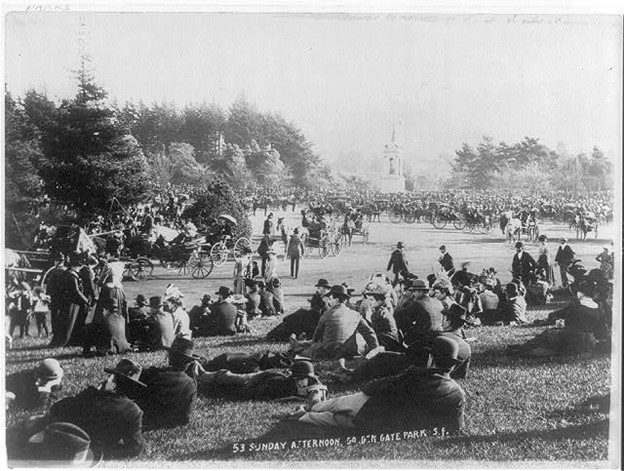
But the systems were not only tools of colonialism. They also grew to support the mundane functions of our daily lives and created the landscapes nearly all of us live in today. Ishi lived his final few years in a San Francisco apartment, in a landscape that had been biologically transformed from just a generation before (Fig. 6.1). He saw imported ornamental plants as he strolled through the city’s planned parks and tended gardens that had replaced the sand dunes and coastal bluffs where the city now stood. Just outside the city, he saw an increasingly cultivated and irrigated landscape of farms and ranches where oak savanna and vast seasonal wetlands had once dominated. He probably did not see elk, grizzly bears, or wolves—species that had once been common in the area. The biological changes Ishi saw in his lifetime only accelerated after his death. In this chapter, I broadly summarize the forces that have been shaping biodiversity patterns during the Anthropocene.
6.1. The Sixth Extinction
Section 1.1: Time Signatures
Biodiversity is constantly being created and destroyed. Sometimes, the destruction outpaces the creation, no more spectacularly so than during mass extinction events. There have been five previous mass extinctions over the period of Earth history, starting with the proliferation of multicellular life that emerged during the Cambrian period. We have strong evidence that Earth is currently experiencing a sixth mass extinction (Table 6.1). Our understanding of what happened during the five previous ones is a bit sketchy. While we are pretty sure an asteroid triggered the Cretaceous-Tertiary extinction, we are fuzzier on the causes of the others. In addition, the patchy and idiosyncratic nature of the fossil record makes it difficult to know what the full impacts on the planet’s biodiversity were, let alone how those changes affected ecosystem functions and processes. Unfortunately, this time around, we are causing this mass extinction and therefore have a firsthand picture of what is going on.
| Summaries of Earth’s Major Extinction Events</th. | ||||
|---|---|---|---|---|
| Mass Extinction Event | Time period (measured in mya–millions of years ago) | Percent of global species eliminated | Possible cause | Notable groups most affected |
| Ordovician-Silurian | 445 mya | 60-70% | A short intense ice age | Marine invertebrates |
| End Devonian | 375-360 mya | up to 75% | Depleted oxygen levels in the ocean triggered by the colonization of land by plants | Marine invertebrates in shallow habitats |
| End Permian | 252 | 96% of marine species 70% of terrestrial species |
volcanic activity | Almost everything. Probably the largest extinction in Earth’s history |
| Triassic-Jurassic | 200 mya | 70-80% | Unclear | Large land animals |
| Cretaceous-Tertiary | 66 mya | 75% | Asteroid impact | Non-bird dinosaurs |
| Holocene-Anthropocene | On going | To be determined, but current extinction rates are comparable to the previous five. | Human modification of the planet | Large vertebrates; habitat or behavioral specialists |
Statistics of Decline
That said, because we are living through this mass extinction in real time, it can be difficult to gain the perspective needed to fully appreciate the scale of the catastrophe. On the face of it, the raw numbers of species that are known to have gone extinct over the past few hundred years don’t sound all that dire. For instance, we definitively know that 338 of the more than 66,000 described vertebrate species went extinct between 1500 and the start of the twenty-first century. If we include species that no one has seen in a long time and are probably extinct as well as species that are only preserved in captivity, then the number increases to 617.5 That expanded number is undoubtedly still an underestimate of actual extinctions since many species have likely gone extinct without us knowing about it, even before we formally named them as species. But to appreciate how alarming these conservative estimates are, we should consider the rate of extinction. Over the whole period of vertebrate evolution, the chronic background rate of extinctions has been 2 extinctions per million species per year.
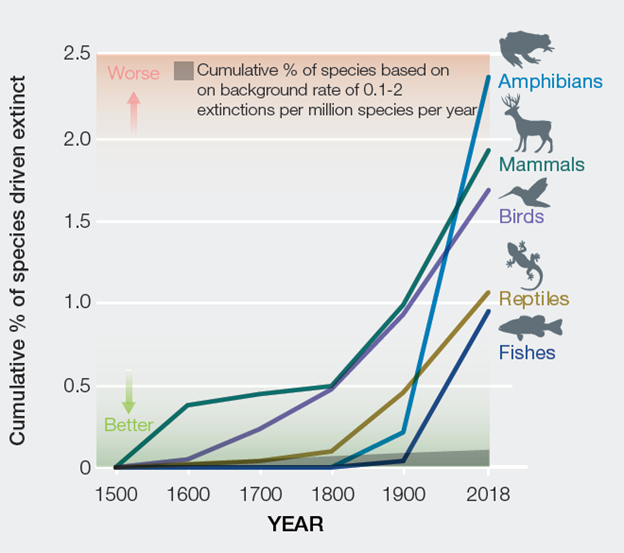
Given that background rate, we would have expected 9 vertebrate species to have gone extinct from 1900 to 2000. Instead, 477 went extinct. That is 53 times greater than the background. Put another way, it would have taken more than 5,000 years for the same number of extinctions to accumulate under the normal background extinction rate. Some specific vertebrate groups are being hit particularly hard. The extinction rate for amphibians, for instance, is 100 times the background. The pace of extinction has also been getting quicker over the course of the Anthropocene, with no sign of leveling off (Fig. 6.2). Keep in mind that these statistics are just for vertebrates, the group of organisms that we know the most about. Plants and invertebrates are experiencing similarly rapid extinctions, although we are less certain about the magnitude. We know the least about microbes, and although we know that their diversity patterns are changing, it is technically and conceptually difficult to assess these changes in terms of species extinction.6
As dire as the extinction rates already are, they will likely get much worse. Extinction is the last stop on a journey of decline that involves diminishing population growth, shrinking population size, and diminishing geographic range. Looked at in terms of these population-level metrics, a shockingly large amount of Earth’s individual organisms have already bit the dust, putting the species they represent in imminent peril. The geographic range of about a third of all the known vertebrate species on Earth have shrunk since 1900. The most complete data we have are for mammals. Of the 177 mammals for which data are available, all have lost 30% or more of their geographic range, and more than 40% of the species have lost more than 80% of their range since 1900.7 The abundance of vertebrates has also declined precipitously, with a mean loss of 68% between 1970 and 2016.8
Think about that last statistic. The abundance of vertebrate animals is now less than one-third of what it was when you or your parents were born. Scientists have bluntly described it as a “biological annihilation.”9 It is not just vertebrates that are running the gauntlet of decline, although the data for other taxonomic groups are less comprehensive. A recent study estimated that the total biomass of flying insects in German nature preserves has declined an astounding 76% over the past 27 years.10
While German hikers might not miss the flying insects all that much, the rest of the food web in which these insects play a central role probably does. Many other abundant, widespread, or otherwise iconic species are experiencing similar declines. Ash trees (Fraxinus spp.) are among the most abundant trees in Northern Hemisphere temperate forests. They provide many valuable ecosystem services, perhaps not least being they are the preferred wood for making baseball bats and hockey sticks. Ash species in both Europe and North America have suffered steep declines, but the crash has been particularly bad in North America. Ash species there have been devastated by a non-native beetle pest, the emerald ash borer (Agrilus planipennis), whose spread and impact have been exacerbated by climate change. Over the roughly 20 years since the beetle arrived, hundreds of millions of trees have died, and five of the most prominent ash species are now listed by the International Union for Conservation of Nature (IUCN) as Critically Endangered.11
The IUCN is the world’s archivist of species decline. They evaluate species for their extinction risk and publish a yearly list of the results called the IUCN Red List of Threatened Species.12 Extinction risk is essentially a function of how widespread and abundant individuals of a species currently are as well as the trajectories of those population metrics. Species that have few overall numbers or are only found in a few geographically isolated populations have a high extinction risk, as do more abundant and widespread species (such as North American ash species) that are experiencing rapid population declines or range contractions. After reviewing the available data for the year, the IUCN assigns species to one of seven risk categories that progressively go from Least Concern to Extinct; there is also a category for species for which there isn’t enough data to evaluate (Table 6.2).
| The International Union for Conservation of Nature (IUCN) extinction assessment categories with example organisms. | ||
|---|---|---|
| Category | Organism Picture | Example Species |
| Data Deficient | 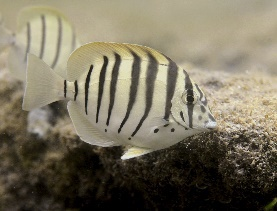 |
Multibar surgeonfish (Acanthurus polyzona)
A reef fish with a restricted range in the western Indian Ocean. We don’t know much about its population ecology. |
| Least Concern | 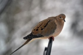 |
Mourning dove (Zenaida macroura).
One of the more widespread and abundant birds in North America. Still, least doesn’t mean no concern; there are reports of recent population declines. |
| Near-threatened | 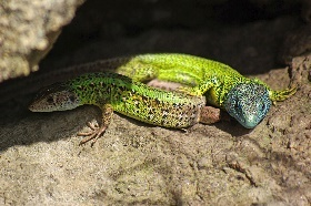 |
Iberian emerald lizard (Lacerta schreiberi)
Restricted to the Iberian Peninsula; populations have been declining. |
| Vulnerable |  |
Rock gnome lichen (Cetradonia linearis)
A lichen from high elevations in the southern Appalachian Mountains. Its habitat is threatened by climate change. |
| Endangered | 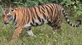 |
Tiger (Panthera tigris)
There are less than 4,000 tigers left in the world. Habitat destruction, hunting, and conflicts with humans are causing their decline. |
| Critically Endangered |  |
White ash (Fraxinus americana)
One of the most abundant and widely distributed ash species in North America. Its abundance is in free fall as a result of the non-native emerald ash borer (Agrilus planipennis) |
| Extinct in the Wild |  |
Guam kingfisher (Todiramphus cinnamominus)
It was eaten to extinction in Guam by the non-native |
| Extinct | 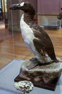 |
Great auk (Pinguinus impennis)
The seabird had been part of human culture in the North Atlantic for thousands of years, but intense hunting starting in the 16th century decimated populations. The last one was seen in 1852. |
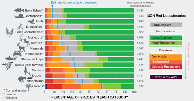
The IUCN Red List is an incomplete picture of how many species are near extinction. In 2021, the IUCN listed 38,500 species as threatened with extinction, 28% of the 138,300 species for which we have detailed ecological information.13 But that well-informed data set is a fraction of the 2.2 million named species of animals and plants, which is itself a fraction of the 8-10 million species that may exist (see Section 2.1). We can use the well-observed patterns to extrapolate reasonable estimates for the actual total number of species that are threatened with extinction (Fig. 6.3). Many groups are under serious threat. For instance, more than 40% of amphibian species and 60% of cycad species are currently threatened. Our confidence in the estimates varies across groups. Insects make up about 75% of all plant and animal species, but we know the least about their extinction risk. A tentative rough estimate from the Intergovernmental Science-Policy Platform on Biodiversity and Ecosystem Services (IPBES) is that perhaps 10% of insects are currently threatened with extinction.14 All together, there are about 1 million (of the estimated total 8-10 million) animal and plant species currently threatened with extinction. That number is weighted heavily in terms of our uncertain estimate for insects.15
Species don’t have to be facing imminent extinction to cause concern. Many still abundant or widespread species are suffering declines. An example is the blue mussel (Mytilus edulis). Blue mussels have not yet been evaluated by the IUCN, perhaps in part because they are abundant and common—or they used to be. In the 1960s, their range extended from the Arctic Sea southwest to North Carolina and southeast to northern Spain. Climate change has contracted their range, however; in the United States, the southern extent of the range has shrunk by 350 km since the 1960s. The overall abundance of mussels across the range has also been in steep decline. In the Gulf of Maine, the average abundance of blue mussels has declined by more than 60%.16
Loss of Functions
When species go extinct, we also lose the ecological relationships they were part of. Extinctions can therefore create changes that ripple through ecosystems and that alter important functions and processes. Loss of function can begin to occur long before the species goes extinct or even before we notice it is threatened. The blue mussel is an example. Individual blue mussels are exceptional filter feeders, and vast colonies of them can filter out prodigious amounts of plankton, making them key parts of shoreline food webs. Collectively, their extensive beds act as strong ecosystem engineers that create habitat for other species. Their decline in abundance is therefore beginning to alter the ecology of North Atlantic coastlines. The relationship between the abundance of individuals and the ecological functions they mediate is often not linear (see, e.g., Fig. 2.19). As a result, ecosystem function can be lost even if a species is still extant but its abundance has declined below some minimum.17 In extreme cases, species can become ecological “living dead” that exist in the landscape as individuals or small groups, but whose broader ecological connections and influence have been lost.18 An example is the American bison (Bison bison). At the start of the nineteenth century, there were an estimated 30-60 million bison; by the start of the twenty-first century, there were only about 4,000. Their functional roles creating soil disturbance, influencing soil nutrient flows, and mediating interactions between prairie plant species have largely been lost from North American ecosystems.19
Blue mussel and bison suggest that the loss of even just a few species that possess particularly important or unique traits could have a dramatic effect on ecosystem processes and the services they generate. Conversely, groups of species that have similar functional traits could provide redundancy that buffers ecosystems from the loss of individual species. As mentioned in Chapter 2, we currently don’t know enough to make comprehensive or detailed predictions about how biodiversity loss will translate into changes in ecosystem function. We also don’t know enough to confidently prioritize which species we should save, as we are forced to do biodiversity triage. But we are making some progress. For instance, increasingly comprehensive and detailed databases describe how species differ in their functional traits. These include characteristics such as what they eat, how they eat, their social behavior, and their physiology. We can use these databases to predict how extinctions would alter the functional traits present in ecosystems. An example comes from a study that looked at large marine animals.20
Large marine animals (marine megafauna) influence the ocean in a number of ways, such as eating prodigious amounts of biomass, transporting nutrients across habitats, and acting as strong ecosystem engineers. Currently, about one-third of the marine megafauna species that the IUCN has evaluated are threatened with extinction. Using models and the IUCN data, researchers estimated that 18% of total megafauna species will go extinct over the next 100 years, assuming their populations stay on a downward trajectory. As a result, functional trait richness will decline by about 11% globally and up to 24% on a regional basis. When researchers more pessimistically assumed that all the currently threatened megafauna went extinct over 100 years, functional richness declined by 48% globally and up to 70% at the poles. The most unique and specialized traits currently in the global megafauna trait toolbox will be disproportionately lost as a result of extinctions.
It might therefore make sense to focus conservation efforts on endangered species that possess the most unique and specialized traits—what are known as FUSE (functionally unique, specialized, and endangered) species.21 The implication in the name is that the loss of these species could light the fuse that triggers a more widespread ecosystem implosion.
Winners and Losers
As was the case during past mass extinction events, the pattern of extinction during this one is not random. Some species seem to be doing just fine and even benefit from the Anthropocene. Many of these are species that have adapted (evolutionarily, behaviorally, or phenotypically) to the new habitats and conditions that have arisen during the Anthropocene. We simply have to look around our farms and cities to see examples. Many of these species are annoying and damaging pests, like rats and mosquitoes. Some straddle the pest-cuteness divide, such as deer and squirrels. Some have become dependent on us (or us on them), such as domestic dogs and wheat.
There are also winners beyond those species that we live in close association with. For instance, cephalopods, the invertebrate group that includes squid, octopus, and cuttlefish, have been experiencing a global boom in population numbers over the past 60 years.22 Cephalopods have a knack for making it through trying times. They are one of the most enduring animal groups on the planet, with a lineage that goes back more than 480 million years, spanning all five of the previous mass extinction events (Fig. 6.4). One potential reason is that many cephalopods have traits that seem to be generally beneficial during rapidly changing and stressful conditions. These include rapid growth rates, short life spans, and broad environmental tolerances. Many other groups that have survived mass extinction events have similar traits, suggesting that it pays to be a jack-of-all-trades during uncertain times.23 Conversely, species that specialize on a specific habitat or on a narrow set of environmental conditions do not do as well. During this mass extinction, specialized species have suffered disproportionate losses relative to more generalist species.24
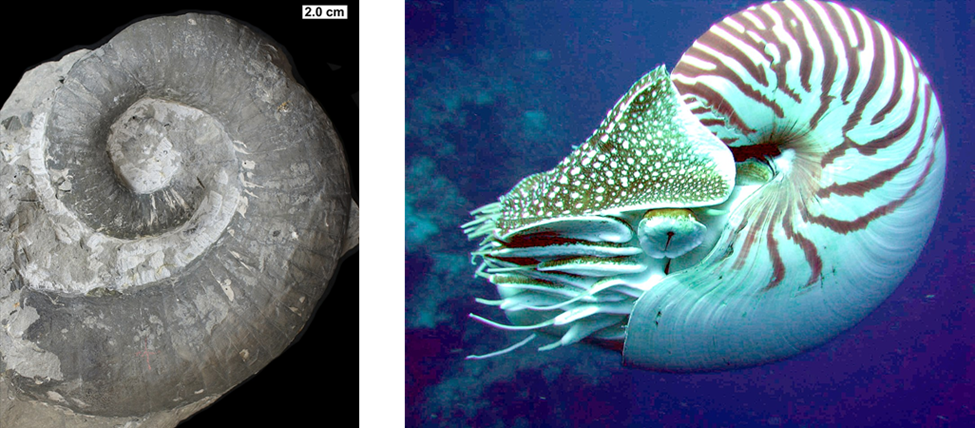
Although being a generalist has clear advantages during a mass extinction, which specific species manage to survive is also often just a matter of circumstance. For instance, like other cephalopods, Nautiloids have survived all five of Earth’s previous mass extinction events (Fig. 6.4). But the modern versions have had the bad luck of catching our eye. Their beautiful shells have made them a target of our intensive fishing. Overfishing has caused several populations in several parts of their range to crash. The fact that they grow uncharacteristically slowly compared to other cephalopods hasn’t helped. They are currently protected under the Convention on International Trade in Endangered Species (CITES) and are listed as threatened under the US Endangered Species Act National Oceanic and Atmospheric Administration.25
Given the primary role that we play in causing extinctions, being attractive to humans is another current extinction risk factor. In many cases, we simply love a species to death. The passenger pigeon (Ectopistes migratorius) was one example. It was one of North America’s most abundant birds, and possibly the most abundant bird species on Earth. Vast, deafening rivers of the birds would darken the sky overhead for hours. Accounts such as this one from Simon Pokagon in 1850 were common:
While I gazed in wonder and astonishment, I beheld moving toward me in an unbroken front millions of pigeons, the first I had seen that season.26
By 1914—65 years after Simon was astonished by their abundance—the species was extinct. The main culprit was our love for pigeon meat. The birds were harvested on an industrial scale, with no regard to what constituted a sustainable harvest. It didn’t help that the bird’s communal social system was uniquely sensitive to reductions in numbers, or that their habitat was also being modified.
There are some other general traits that are proving risky during this mass extinction. These include having a low reproductive rate; having a large body size; requiring large individual home ranges; and inhabiting a small, restricted species range.27
6.2 A Great Reorganization
Section 6.2: A Great Reorganization
Extinctions have become emblematic of our detrimental influence on the planet. It is understandable that we tend to view our relationship with biodiversity almost entirely through the lens of loss. But extinctions are just one aspect of our comprehensive and radical reorganization Earth’s biodiversity. Through the processes described in the rest of this chapter, humans are changing all the different classes of biodiversity (genetic/species, functional, ecosystem) across scales of space and time. We are substantially reducing the biodiversity of many metrics at many scales, but we are also increasing the biodiversity of other metrics at other scales. We are breaking up old associations, disrupting long-term relationships, and destroying established patterns of life, but we are also creating entirely new associations, building new relationships, and catalyzing new patterns of life. It is difficult to grasp the scale, magnitude, and speed of these changes, let alone understand them. But we have begun to develop a rudimentary picture of what is going on.
Five broad patterns are emerging:
- Biodiversity is declining at the global scale.
- Biodiversity is both increasing and decreasing at smaller spatial scales.
- Novel associations of biodiversity are forming, and old associations are being lost.
- Biodiversity is tending to become more homogenous across space.
- The pace of change is increasing.
Although all the classes of biodiversity are changing, the best information we have gathered so far is for species (Table 6.3). The table shows two different metrics of species diversity: species richness and species turnover across space. The rows are three different spatial perspectives: a local patch, a broad region, and the entire Earth. See section 2.1 for more on the metrics and the scales at which we can observe them. As the previous section described, we are losing species to extinction at an alarming rate. The extinctions are unambiguously reducing species richness at the global scale.
| Average Species Richness and Turnover at Three Spatial Scales | ||
|---|---|---|
| Spatial Scale | Species Richness | Species Spatial Turnover* *change in species across space |
| Global | Lowering | We only have one Earth, so there can be no turnover. |
| Regional | Rising | Lowering |
| Local | Remaining Stable | Lowering |
At smaller spatial scales, however, things are a bit more complicated. The number of species in any given area at any given time is the balance of species losses and gains. Species are lost when they get locally extirpated or move away from an area. Species are gained when they colonize an area. We are currently the main driving agent behind both the losses and gains:
- We extirpate populations through a variety of activities (see the end of this section).
- Climate change (see Chap. 5 and section 6.3) and ecosystem domestication (section 6.4) cause species to shift their ranges out of some areas and into new ones.
- We actively transport organisms (intentionally and unintentionally) from their original natural range to new areas (section 6.5).
At regional scales, the loss of species has tended to be more than compensated for by the arrival of new species, so that species richness has been trending upward in many regions. Isolated oceanic islands exemplify this phenomenon. Oceanic islands have lost a significant number of their original species. For instance, in the years since Europeans arrived in the Hawaiian Islands, approximately 23 native Hawaiian land bird species have gone extinct. But 55 species have been introduced, so the local bird species richness of Hawaii has actually increased since the arrival of Europeans. This pattern is even more striking for plants, as 71 species have gone extinct compared with 1,090 (and counting) that have been added to the Hawaiian flora, mostly since European colonization.28 The pattern is similar across all oceanic islands: land bird extinctions have roughly been balanced by new colonizations, while many more plant species have colonized than have gone extinct.29
A potential reason for why species are accumulating within regions is that we are still in the early stages of extinction. While the abundance of many species has declined, they can still show up on the regional species checklist. The vaquita (Phocoena sinus)—the world’s smallest cetacean—is still on the species list for the Gulf of California even though there are fewer than 10 of them.30
Plants are particularly good at tenaciously hanging on. For instance, adult trees can live for hundreds of years even if conditions have halted the recruitment of seedlings. Species can also adapt to changing conditions in various ways, allowing them to persist (see Chapter 5 for examples of how species are adjusting to climate change). At the same time, the processes adding species to regions such as climate-change-driven range shifts and our direct movement of species have been accelerating. For instance, we have been introducing new fish species to the Seine River in northern France for a long time. The first documented introduction was common carp (Cyprinus carpio) in the thirteenth century, but it wasn’t until the mid-nineteenth century that fish introductions began to gather steam. The pace picked up dramatically starting in the middle of the twentieth century and has been accelerating in recent years. By the start of the twenty-first century, an average of four new species were establishing in the Seine every decade. As of 2020, 46% of the species found in the Seine were not originally native to the region.31
There is a similar pattern at the scale of a local patch. Some species are dropping off local species checklists while new ones are being added. The net result at these smaller spatial scales seems to be more variable than for larger regions. On average, the species richness of local patches hasn’t changed in any systematic way over the past couple hundred years; the number of individual locations that have lost net species has been roughly balanced by others that have gained net species.3233That seems to reflect the idiosyncratic ways our activities interact with local circumstances. For example, local plant species richness in California grasslands declined from 2000 to 2014, likely as a result of decreased rainfall over that period. In contrast, local plant species richness in the forest and grassland habitats of Vancouver Island, Canada, increased from 1968 to 2009, mostly because increased human disturbance facilitated the colonization of disturbance adapted species.34
All the reshuffling of species is rapidly changing the species composition of locations around the world. An indication of how widespread the reorganization has become comes from a study that looked at a large database of long-term species inventories at both marine and terrestrial sites around the world. The collection contained more than 50,000 time series of species composition change. Based on these records, the authors of the study estimate that a median 28% of all local species are being replaced by new species every decade.35
The species reshuffling is also tending to smooth out differences in species composition between different locations. Species are expanding their range into new areas while persisting in many parts of their old range. At the same time, many unique endemic species are being lost from locations and regions. As a result, species spatial turnover (i.e., the degree to which the composition of species changes from spot to spot across a landscape) has been declining. The homogenization is evident both across regions and across local patches within a region. Hawaii’s birds are an example of regional homogenization. Hawaii’s extinct birds were all endemic to the archipelago and represented unique genetic and phenotypic types that were found nowhere else in the world. In contrast, the new colonists have been mostly generalist species that are found in many other regions across the Pacific and the world. Hawaii is now a bit more like every other island archipelago on Earth in terms of its birds.
We don’t have as much data for the other classes of biodiversity (population-level genetics, functions, and ecosystems) as we do for species. But the data that we do have suggest that they are changing in broadly similar ways, although the details vary across the classes and spatial scales. For example, climate change combined with landscape changes such as dams and the loss of riparian vegetation have caused river systems around the world to get warmer and slower over the past 40 years or so. As a result, rivers have become increasingly dominated by species adapted to warm, slow conditions. Rivers are now much more similar to each other in terms of the fish functional traits related to temperature and water flow.36
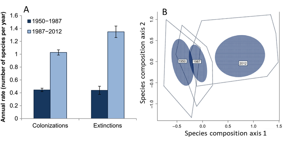
Like the other indicators of the Anthropocene, biodiversity change has been accelerating since the 1950s. The plant species found in patches of Wisconsin prairie provide an illustration.37 Consistent species inventories began in 1950. Since then, the composition of the patches has changed as some species went locally extinct and others colonized. From 1950 to 1987, extinction and colonization were roughly balanced. Over that period, species richness stayed about the same while the collective species composition began to modestly shift. The turnover of species picked up dramatically from 1987 to 2012. Annual extinction rates increased by 214%, and annual colonization rates increased by 129% compared to the 1950-1987 period. The species composition has also diverged dramatically from what it was in 1950. While patches still have about the same number of species (or slightly more) as they had in 1950, the identities of the species are different (Fig. 6.5). Some local patches now have fewer than 18% of the specific species they had in 1950. Most of the new colonists to the patches have been non-native species that we introduced to the region. The accelerating rate of these introductions has been a big reason for the increased pace of change. Other drivers of change include changing fire patterns as well as our continued reductions to the size of some of the patches.
Drivers of Change
There are five main processes that are driving the changes to Anthropocene biodiversity:
- Climate change
- Ecosystem domestication
- Human-assisted species movement
- Overexploitation
- Pollution
These processes tend to directly counter many of the forces that generate and maintain biodiversity described in Chapter 2. They tend to break down isolation between populations, they tend to impose strong uniform selection that favors a few life history strategies, they tend to homogenize abiotic conditions and resource availability across space and time, and they tend to create disturbances that maintain ecosystems in states of early succession. A complicating factor is that the five main processes interact across scales of space and time. For example, the land use changes associated with our domestication of tropical forests have directly contributed to biodiversity loss. They have also switched many tropical forests from being a significant sink for our greenhouse gas emissions into being a significant net source of greenhouse gas emissions of their own.38 That in turn could accelerate global warming and lead to even more extinctions. I briefly discuss these important interactions in Section 6.8. But for the sake of sanity, let’s first explore each of the drivers separately.
6.3 Climate Change
Section 6.3: Climate Change
In Chapter 5 I described the main ways that climate change and the associated decline in ocean alkalinity are reorganizing the biosphere, so I won’t rehash those details here. But given the ongoing and predicted changes to the distribution and abundance of organisms that both climate change and ocean acidification are causing, there are clear reasons to suspect that it will contribute to biodiversity loss. As local climates shift, extreme or particularly unique ecosystems such as those in the cryosphere will likely shrink and in some cases disappear altogether. Similarly, some species will not be able to adapt (behaviorally, physiologically, evolutionarily) quickly enough before climate change eliminates their ecological niche. Some will fall victim indirectly when the species they depend on for food, for pollination, for dispersal, or for the creation of the habitat they live in decline in abundance or go extinct. As species ranges shift, a measure of the unique biodiversity of places will likely get lost as regions are homogenized and increasingly dominated by the generalist species that are most adept at weathering change. The movement of species will also create novel interactions that in some cases will result in reduced local diversity, as has been the case with the poleward expansion of tropical herbivorous fish (see Fig. 5.9). At the level of populations, the rearrangement of populations across a landscape will in some cases reduce their net isolation, causing reduction in genotypic and phenotypic diversity.
A recent review of published studies concluded that one in six terrestrial species face an elevated risk of extinction if climate change proceeds on current trajectories. Similarly, a review of 632 published experiments suggests that ocean acidification will likely cause broad reductions to marine diversity as well as an overall simplification of marine trophic structure.39
Despite clear evidence that climate change has had significant impacts on species and ecosystems, we don’t yet have unambiguous evidence that any extinctions have occurred as a direct result of climate change.40 This is partly because most extinctions reflect a complex chain of causality, and it is difficult to disentangle the role each cause plays. But also, compared to some of the other drivers of biodiversity change, climate change is just starting to get into gear, and many of its impacts won’t be seen until sometime into the future. For instance, the 1.2°C that we have already warmed the planet above preindustrial levels (as of 2020) may cause 3% of the world’s species to go extinct; we just haven’t seen the extinctions yet because of time lags in how populations respond to climate change.41 The future-pointing orientation of climate change adds a level of uncertainty in understanding its impacts. It also provides a level of hope that we could still significantly mitigate future climate change and its impact on biodiversity.
6.4. Domestication
Section 6.4: Domestication
If climate change is the future threat to biodiversity, domestication is the clear past and present danger. You probably think of domestication in terms of the plant and animal species we have bred as biological tools and companions. That is part of it (see below), but domestication is a broader system that has allowed us to radically reshape the planet, and it—perhaps more than anything—defines the Anthropocene (see Chap. 3). Many of the ecosystem changes that I outline in Chapter 3 are the direct result of deliberate modifications designed to provide us with diverse and reliable supplies of food and fiber, warm and clean living spaces, and a sense of connection and companionship with the natural world in those human spaces. In short, we have domesticated large swaths of the planet. Domestication in this sense involves two broad processes that influence biodiversity patterns.
Conversion to Anthropogenic Ecosystems
As I describe in Chapter 3, 75% of Earth’s land surface is now occupied by anthropogenic ecosystems (anthromes) whose abiotic and biotic components we have deliberately modified to serve us. In the most extreme cases, we have wholly replaced ecosystems with ones that are almost completely of our own design and management. Examples are our intensive agricultural systems and our cities, which combined now make up about one-third of the ice-free land surface (see Fig. 3.20). The creation of these ecosystems often (but not always) reduces biodiversity at some (but not all) scales. A simple explanation for this is that when we create these ecosystems, we largely destroy the existing biodiversity and replace it with something less diverse, like a parking lot or a crop field. The conversion of tropical rainforest into agro-ecosystems is a good example (Fig. 6.6).

The tendency of our domesticated landscapes to support less biodiversity is related to the often narrow goals we have for them. These usually involve supporting our own well-being and benefitting the few species that we directly depend on or care about. We finely tune environmental conditions to optimally support those goals, and we make these optimal conditions as homogenous in space and time as possible. For example, farming practices (e.g., tillage, fertilizers, irrigation) are an attempt to create and maintain optimal conditions for crops. The narrow set of conditions and their homogeneity in space and time that we develop in our domesticated ecosystems are the direct opposite of the variable conditions and heterogeneous resource patterns that foster and maintain biodiversity. Think about this in terms of the niche complementarity model described in Figure 2.9. In that model, variability in resources allowed species with different niches to coexist. By creating a narrow and homogeneous set of conditions, we effectively shrink the potential niche space (the size of the box in Fig. 2.9) available to species. Our conceptual goal is often to make the size and shape of the potential niche space exactly the size and shape of that for a single species such as maize or soybean. Of course, we can’t practically achieve that. Still, we have been able to make many of our farms and cities remarkably uniform in terms of abiotic conditions. On top of that, we use disturbance to constantly reset the system if it ever starts to diverge from our narrow goals, perpetually keeping these systems in a state of early succession.
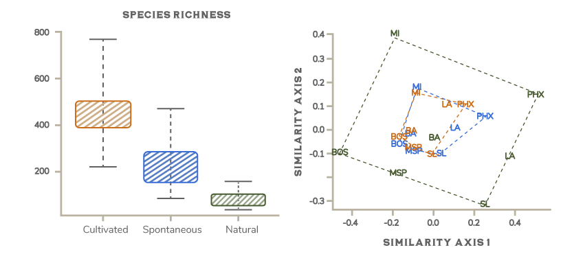
That simple explanation is too simple, however. Although some domesticated landscapes are nearly devoid of life (e.g., parking lots), most support more diverse communities of organisms that form complex biodiversity patterns. Urban landscapes are a good example. We have designed our urban landscapes using a diverse pallet of domesticated horticultural species drawn from disparate ecosystems and from nearly every corner of the world. In addition, urban environments support species that have escaped cultivation as well as species that have colonized urban environments from the local surrounding region. As a result, urban landscapes often have more total plant species than nearby natural areas (Fig. 6.7A). But people around the world have similar goals for their urban landscapes, and these get reflected in similar designs. In addition, the global trade in ornamental plants and management tools such as irrigation allows us to implement designs using similar sets of species no matter what the local conditions are. The net result is that although urban florae are species-rich, they tend to be relatively similar to each other compared to the natural florae in their respective regions (Fig. 6.7B). For instance, the Sonoran Desert and eastern deciduous forests share hardly any plant species in common, but the residential yards of suburban Phoenix and Boston have quite a few plant species in common.
Anthromes are more complex than simply industrialized farms and cookie-cutter cities. There is (ironically) a lot of diversity in how we manage our domesticated ecosystems, the degree to which that management modifies abiotic and biotic conditions, and the impact that has on specific components of biodiversity. In some cases and at some scales, the impacts on biodiversity can be positive. In fact, several anthromes are considered valuable contributors to biodiversity. A good example is the cork oak ecosystem of the western Mediterranean Basin (Fig. 6.8). These anthromes have been actively managed by humans for millennia to provide cork, pastureland for grazing animals, habitat for game animals, and cropland. Perhaps because of these diverse uses, cork oak landscapes are a complex patchwork of abiotic conditions, states of succession, and habitats. These in turn foster a rich assortment of plant and animal species, including many endemic species as well as many now-threatened species such as the Iberian lynx (Lynx pardinus). But this condition is sensitive to the type of management we apply. In the absence of active management, principally in the form of grazing by domesticated animals, shrubs slowly replace the open grassland components of the system. This creates a more uniform woody vegetation that has lower biodiversity at the regional scale. In contrast, other types of management reduce biodiversity such as overgrazing and the replacement of oak trees with more intensively managed crops such as citrus.
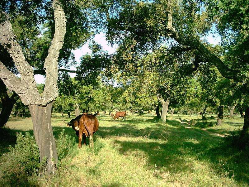
Many other landscapes follow a similar pattern to the cork oak example: just the right type and amount of human management maintains and sometimes enhances biodiversity and ecosystem services. In many ways, this fact has become a guiding principle for resource managers and conservation biologists, and it provides hope that we can find a sustainable balance of biodiversity and human use. One big roadblock is that management decisions are often more influenced by social and economic forces than they are by the goals of optimizing biodiversity or providing a diverse suite of ecosystem services. For instance, cork oaks in the region are being replaced by citrus partly because the demand for cork has been declining as the wine industry turns to other materials for their stoppers. For more on valuing ecosystem services, see section 2.5.
Despite examples like cork oak ecosystems, our creation of anthromes has in aggregate been reducing biodiversity. This is mostly a result of the social and economic changes associated with the Great Acceleration that have caused us to convert a vast amount of land into low-diversity systems like row crops. One estimate is that, on a global average, our creation of anthromes has reduced local species richness (the number of species in a patch of land) by 14% and the abundance of those species by 11%.42 The authors of that study predict that given current trends in our land use, local richness will fall an additional 3.4% by 2100. Those average estimates blur a lot of variation. Unhelpfully, regions that are currently experiencing the greatest expansion of intensive human ecosystems are also the regions with the highest levels of existing biodiversity, such as tropical forests and Mediterranean-type ecosystems.43
Selection, Breeding, and Genetic Engineering
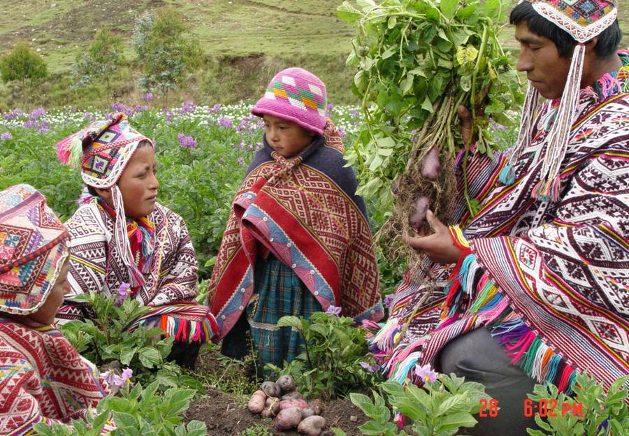
The development of domesticated animals and plants through the directed selection of desirable types and planned breeding to create new types was a critical step in the development of agriculture. Initially, selection and breeding were relatively localized activities. Individual communities and in some cases even individual households developed their own unique varieties of crops and animals that were tailored to their specific local abiotic conditions, diseases, tastes, and ways of farming. We have created quite a few of these landraces, as they are called. A classic example is cultivated forms of potatoes (Solanum tuberosum and a few other Solanum species), which were first developed from wild forms in the Andes of southern Peru 8,000–10,000 years ago. Today there are more than 4,000 different potato varieties. Most of these have been developed by Andean farmers (Fig. 6.9), but farmers around the world have also developed their own local landraces.44
From one perspective, the efforts of potato farmers and breeders have increased the world’s biodiversity. Selection, breeding, and more recent genetic engineering tools directly create new phenotypes and genotypes. As with broader ecosystem domestication, however, things are more complex than that one perspective. There are more than 100 wild potato species that in aggregate span a geographic range from North America to the tip of South America and that inhabit a diversity of environments. But all the current domesticated types descend from just a few (perhaps a single) progenitor wild species. As a result, the collective genetic diversity of domesticated potatoes is a small fraction of the genetic diversity found in wild forms. That reduced genetic diversity translates into reduced phenotypic diversity for some traits. For instance, wild potatoes have much more diverse genes associated with disease resistance than do cultivated potatoes.45 The loss of genetic and phenotypic diversity has only gotten worse as we continue to breed potatoes. The main potato varieties grown in North America are all derived from a few European and Chilean types that survived the Irish potato famine of the 1840s.46
A similar filtering process has occurred for all domesticated crops. In addition, as we got better at regulating the abiotic conditions on farms, we increasingly tailored our domesticated species to benefit from those conditions. Breeding and the creation of anthropogenic ecosystems positively feed back on each other. We design ecosystems to benefit our favorite species, and we design species to make the most out of the ecosystems we design for them. Farmers around the world have been creating ever more similar agronomic environments, and as a consequence, the traits and characteristics they want in the organisms they grow or husband have been getting more similar. The other drivers of the Great Acceleration such as globalized markets and global social connectivity have also contributed to reducing crop diversity. Farmers around the world want varieties that ship and store well, are resistant to a similar list of pests, and that are favored by similar groups of consumers with similar diets and tastes. This has tended to reduce trait and functional diversity within our domesticated species. There is concern that these narrow selection goals are steadily eroding the genetic diversity of crops—the very diversity that is needed to select and breed new forms in the first place.47 At the same time, the diversity of the wild relatives of many crops is threatened by our creation of anthropogenic ecosystems. For instance, the IUCN has listed three species of wild rice, two species of wild wheat, and seventeen species of wild yam as threatened by the spread of anthropogenic ecosystems.48
As is always the case with biodiversity, the scale and type of diversity you focus on can change your perspective. Since the 1960s, the number of different food crops that people eat locally (local diet richness) has steadily increased. This reflects the increase in our overall prosperity as well as the development of a global food system. You can now buy a cheap banana nearly any place there are humans in the world, but just a century ago, many people had never seen a banana, let along packed one in their lunch box on a regular basis.49 One consequence of the global spread of once-regional foods along with the spread of food cultures and traditions is that diets and the types of crops we all rely on have been steadily getting more similar from region to region around the world.50 From a risk management standpoint, this is troubling, as only a few major crops running into trouble (e.g., from disruptions caused by climate change) can have a massive impact on global food security.
6.5 Human-Assisted Movement
Section 6.5: Human-Assisted Movement
As our ancestors migrated out of Africa, they undoubtedly brought other species along with them. We have evidence that at least a few parasites and disease-causing microbes did.51 But our knack for transporting organisms around the globe didn’t really develop until the agro-industrial revolution.52 As I describe in Chapter 2, the planet’s geographic barriers had been enough to keep most organisms isolated from each other for long periods. The spatial arrangement of those isolating barriers has been an important factor shaping Earth’s biodiversity patterns (see Fig. 2.8). Since the agro-industrial revolution, we have made those barriers decidedly less formidable. The landscape you are sitting in as you read this is probably full of species that mostly evolved someplace else and arrived in your region within the past 200 years with human help.
When we move organisms, we potentially create three classes of the populations that compose a species (Table 6.4). There are a confusing number of synonyms used to describe these three classes of populations. Also, it is more common to use the terms native species, non-native species, and invasive species instead of native populations, non-native populations, and invasive populations. I will also frequently use such phrasing. But you should keep the distinction in mind. At any given time, a species can be simultaneously composed of different populations that are native, non-native, and invasive.
Types of Populations, A Short-List
| Term | Definition | Ambiguities |
|---|---|---|
| Native Populations | Synonym: indigenous | Species ranges are naturally dynamic and can expand or contract without our direct help. |
| Populations of a species occupying a natural geographic range unassisted by humans. | ||
| Non-native populations | Synonyms: alien, non-indigenous, introduced, exotic | Populations that have been intentionally or accidentally moved by humans outside of the natural range of their species. The non-native populations can be self-sustaining or require constant human intervention to maintain. Human activities such as climate change and habitat change can indirectly trigger the natural dispersal of organisms into new areas.
We introduced some populations a long time ago (hundreds to thousands of years ago) and now sometimes consider their human assisted range as natural. |
| Invasive populations | Synonyms: noxious, weedy, nuisance | Non-native populations that are self-sustaining, that have spread some distance from their initial introduction site, and that have the potential to spread widely or become super abundant without further human intervention.
The demarcation between self-sustaining non-native populations and invasive populations is dynamic and fuzzy. The definition intentionally excludes any mention of how the populations alter ecosystems or ecosystem services (i.e. their impact). But in common usage the term often implies strong impacts (e.g. see the synonyms). |
We transport organisms in two broad ways.
Intentionally
We intentionally move organisms to provide various functions and services. Many of these are domesticated species that rarely move beyond the limits of the domesticated ecosystems we create for them. But some domesticated species do venture out on their own to establish self-sustaining populations. These tend to be organisms that have only been slightly modified from their wild forms or that have been selected for traits such as broad environmental tolerances that help facilitate their autonomous spread. Many ornamental plant species fit that description, and in many regions, most non-native and invasive plants are escapees of cultivated ornamentals that were imported via the horticulture trade.53 In other cases, non-native populations of domesticated species exist in a gray area between dependence and independence from us. Classic examples are domesticated dogs and cats whose free-roaming and feral populations have become important new predators in many ecosystems.5455
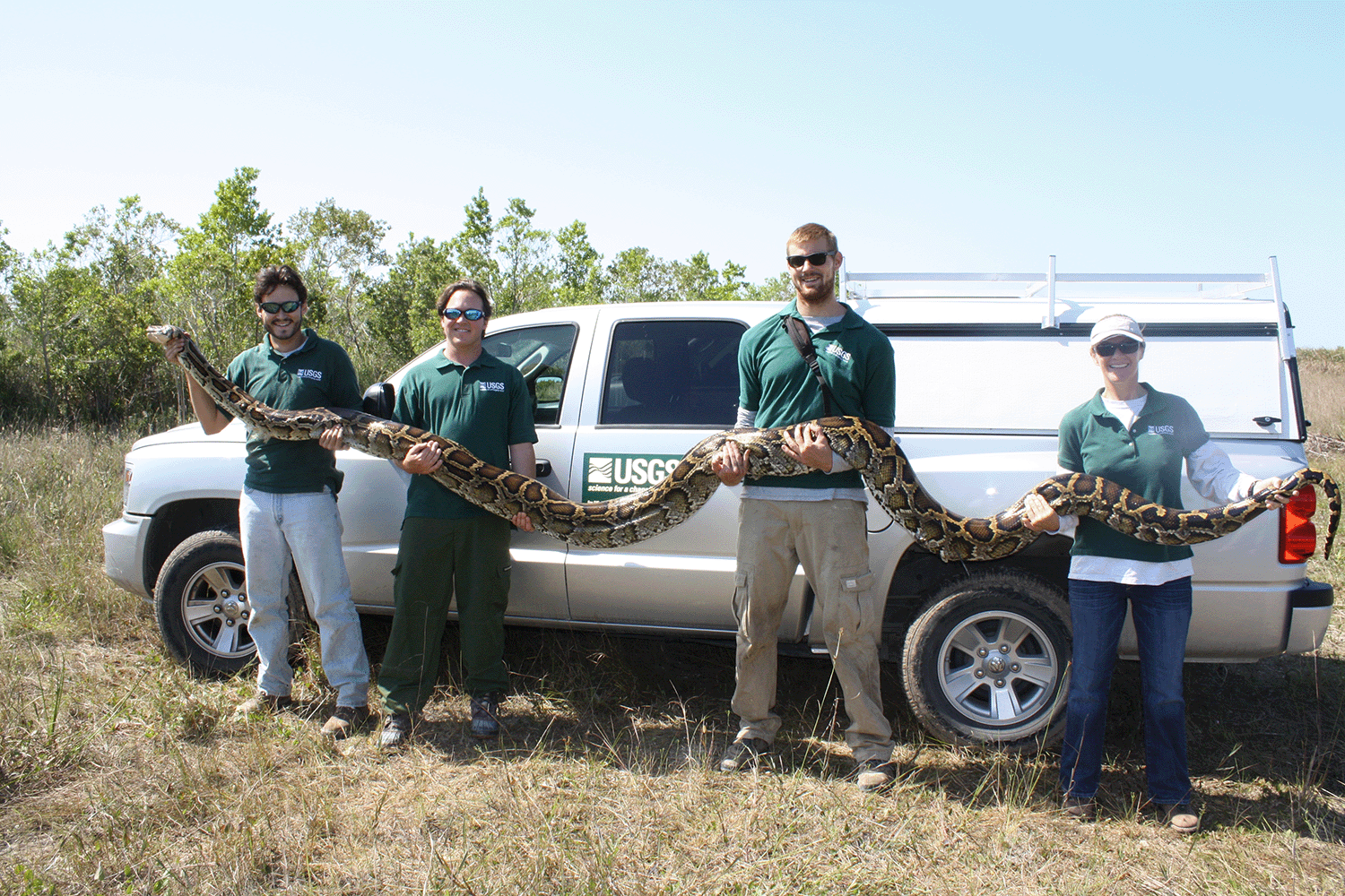
Sometimes, we intentionally spread wild species. Eugene Schieffelin gave us a notorious example when he introduced European starlings to New York’s Central Park in 1890.56 Schieffelin wanted to improve the social (and presumably natural) culture of North America by introducing all the birds mentioned in the plays of William Shakespeare. This pathway of spread did not stop with Eugene Schieffelin. Wild-caught species have now become a significant part of the global pet trade. That trade directly influences biodiversity in the regions where the animals are caught (see section 6.6), but in addition, many of the wild pets subsequently escape or are intentionally released to become serious pests in their new homes.57 That is how Burmese pythons (Python molurus bivittatus) became part of the reptile fauna of the Florida Everglades (Fig. 6.10).
Accidentally
The other main way we move species around is accidently. The number of non-native populations has been accelerating since 1950, primarily as an incidental result of increasingly connected and efficient global transportation networks.58 We can get to the remotest parts of the planet within a matter of days and to most places within a matter of hours. So just about any species can now hop aboard a plane, find a quiet spot in a shipping container, or cling to the clothes of intrepid backpackers (to mention just a few of the known introduction pathways).
Many of these species have evolved to take advantage of these transportation networks or the created ecosystems the networks connect. The numerous introduced organisms that cause human diseases or that have become pests in agricultural and urban ecosystems are prime examples. Other introductions are truly accidental. These accidents have always happened naturally without our help. Creosote bush (Larrea tridentata) is now an iconic species in the warm deserts of North America. It is hard to imagine these deserts without creosote bush, but genetic evidence suggests that creosote bush is a relatively recent arrival to North America, perhaps sometime in the Pleistocene or late Pliocene.59 It somehow dispersed from populations of its closely related sister taxa L. divaricata in South America. Migratory birds that regularly fly between North and South America are suspected to have caused the introduction. In sharp contrast to those rare natural accidents, we have made the accidental movement of organisms as common as the next arriving flight or port of call.60
Effects on Biodiversity
Our movement of organisms is profoundly reorganizing the biodiversity of the planet. One study estimated that as of the beginning of the twenty-first century, humans had transported about 14,000 plant species that had established self-sustaining non-native populations, about 4% of all the known plant species.61 We have translocated similar proportions of other groups, including fish (5%) and birds (3%).6263
As I describe in section 6.2, one result of these introductions has been to increase species richness at many local and regional scales but to decrease local and regional uniqueness as species become more homogenized across space. These contradictory effects play out in a wide variety of ways in different ecosystems and groups of organisms, they vary across different spatial scales, and they can change over time.
In addition, non-native populations do more than just add a line to a species checklist. Non-native organisms interact with resident organisms and with the abiotic parts of their new ecosystem. Just like when I was sent away to summer camp, the process of forming new relationships, integrating into the local community, and adjusting to a new environment can be traumatic and transformative for everyone involved. These new ecological interactions can sometimes profoundly alter the functioning of ecosystems, which in turn can further change biodiversity patterns and alter the services that ecosystems provide.
As with biodiversity change in general, we don’t have a complete picture of the ways non-native populations are altering biodiversity. We also don’t understand how the initial changes we are observing now will play out as the Anthropocene progresses. But we do have a good understanding of the main ways non-native populations can alter biodiversity and ecosystem functions. There are three of them.
They Interact with Native Populations
Native and non-native populations interact directly with each other. On the face of it, these interactions would seem to pose a significant barrier to any non-native populations getting established in the first place. When they arrive, non-native populations must compete for resources, avoid getting eaten, and establish positive relationships with other species to meet basic needs like pollination. Native populations have the key advantage of being particularly adapted to the ecosystems they are part of. Even if the non-native populations come from a similar climate, there will always be a long list of environmental differences that should give resident species a competitive advantage over non-native populations. Native predators would also seem to have the home field advantage against disoriented new colonists. Plus, native populations won’t persist long if their individuals can’t find a pollinator or the particular type of food they require. There is evidence that these barriers are indeed steep. A rough estimate is that only about 10% of non-native populations manage to form self-staining populations, and a similarly small fraction of those turn into invasive populations.64 There are a few traits and circumstances that can sometimes give non-native populations an advantage, however. These advantages also shape how self-sustaining and invasive non-native populations influence biodiversity.
In some cases, the lack of coevolved relationships with native species can give non-native populations a decided advantage. This idea forms the leading hypothesis for why some non-native populations become invasive: the enemy release hypothesis. The gist of the idea is that in leaving their native range, non-native populations also leave behind a long list of coevolved predators and competitors that kept their growth in check. While the new competitors and predators that non-native populations face will sometimes have home field advantage, they just as often will be ill adapted to handle the newcomers or just ignore them altogether. As a result, the overall collective impact of native predators and competitors on non-native organisms can be much less than what they faced back in their native range. So much less that the non-native populations experience a demographic explosion. The sheer numbers and biomass that result can monopolize resources such as nutrients and space, and this can have a negative effect on local and regional diversity.
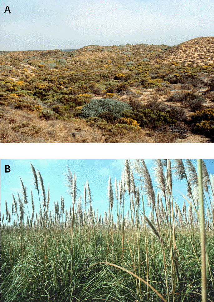
For example, jubata grass (Coretaderia jubata) is a large, showy perennial grass native to the Andes. In its native range, jubata grass is found mostly as scattered individuals and small populations. It was introduced to California in the nineteenth century, and it subsequently escaped cultivation to establish populations along the West Coast of the United States. In contrast to its native range, many of these populations are large and dense. In some places, jubata grass has formed dense stands in areas that once supported rich assemblages of native plant species, many of which are unique endemics (Fig. 6.11).
Non-native populations can also sometimes possess a trait or function that becomes a superpower in their new range because the resident species are unprepared or ill-suited to deal with it.65 A classic example are island birds who because of their isolation had never experienced nastily evolved predators such as cats, snakes, or humans. When they did encounter predators, the results where disastrous for the birds and a bonanza for the predators. This interaction has been a major contributor to the oceanic island bird extinctions mentioned in section 6.2. When the brown tree snake (Boiga irregularis) accidentally arrived on Guam in the 1940s (probably in shipments of US military supplies), it promptly proceeded to eat its way through the island’s birds. It ate to extinction 10 of the island’s 12 native forest bird species. The remaining 2 species have so few individuals that their ecological roles and functions have been effectively lost.66 The snake also ate through the island’s bats and reptiles so that most forested areas on Guam now only have three native vertebrates, all small reptiles.67
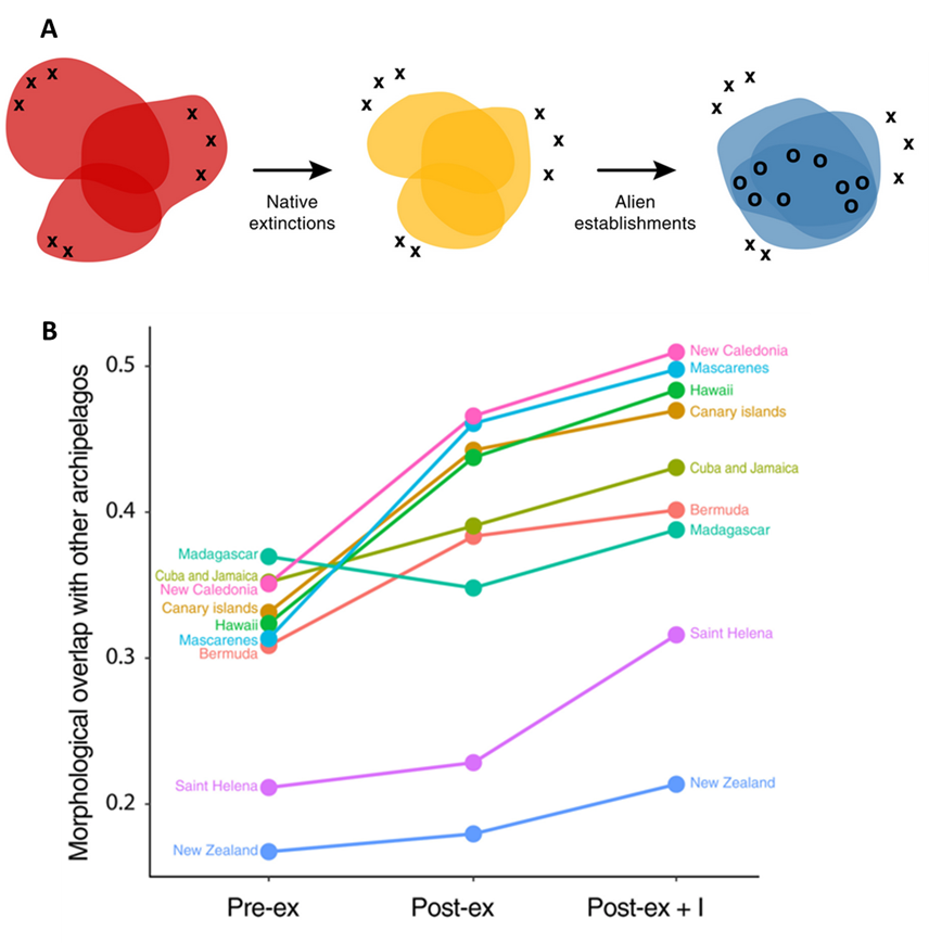
Many non-native populations are successful because they have qualities that serve travelers well: they are adept and dispersing, they are adaptable to new conditions and making new relationships, and they don’t require any specialized conditions. Many are also well adapted to the conditions found in anthropogenic ecosystems. In some cases, those same conditions are negatively affecting native species that would otherwise pose a barrier to new colonists. For example, physical disturbances can (at least temporarily and locally) create windows of opportunity that allow non-native populations a chance to get established and spread.68 In many ecosystems, the level and nature of disturbance have been significantly altered by our actions (see Chap. 2), and the alterations sometimes favor the life history of the non-native species over native species. Consequently, as a group, non-native populations around the world tend to share far more functional similarities than do the species in the resident communities they are joining. This combined with the extinction of endemic and locally specialized species is a major force spatially homogenizing ecosystem characteristics. Birds on islands provide an example. The history of the Hawaiian bird fauna mentioned in section 6.2 is part of a larger pattern on island archipelagos around the world. Island bird faunas are becoming functionally more similar as they lose unique specialized species and gain functionally generalized species that share traits with many other species that have colonized many other islands (Fig. 6.12).
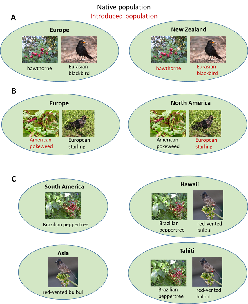
Species introductions are not only homogenizing functional traits; they are also reorganizing the network of relationships and interactions that link species. We have developed a detailed picture of this effect for the mutualistic relationships between fleshy-fruited plants and the animals that eat the fruit and disperse their seeds (frugivores). These are critically important relationships that drive the evolution of species traits, shape biodiversity patterns, and help regulate a broad array of ecosystem traits and functions.
Much like how human social networks are structured into clusters that reflect familial relationships, where we live, and shared interests, plant-frugivore networks are structured into clusters that reflect evolutionary history, geographic location, and environmental circumstances. The global spread of non-native species is smoothing out differences and eroding the unique clustering of regional networks across the globe. In the recent past, local and regional networks were mostly composed of interactions between native plant and animal species. Now they increasingly involve pairs of non-native species. In addition, the same relationships between the same pairs of species are being replicated across regions (Fig. 6.13).
A study that analyzed data on the interactions between 1,631 animal and 3,208 plant species around the world found that the proportion of interactions that involve non-native species is now (in 2020) seven times greater than it was in the 1950s. Not only is the rate of new non-native interactions accelerating, but also non-native animals preferentially form associations with non-native plants, creating a feedback that leads to more homogenization across regions.69
In extreme cases, non-native relationships have completely replaced the old native ones. On Oahu, Hawaii, 93% of the seed dispersal network is now composed of novel interactions between non-native birds and non-native plants. The rest of the interactions are between native plants and non-native birds. Even though researchers spent three years sifting through nearly 3,500 fecal samples and looking at 5,000 camera trap images, they didn’t record a single interaction between a native bird and a native plant.70 Other islands have been even more affected because non-native animals have not replaced the seed dispersal functions for native plants. Guam is one such case. When the brown tree snake ate the island’s native vertebrates, the native trees lost their specialized seed dispersal partners. As a result, native trees have suffered up to 92% declines in recruitment.71 Although no tree species have yet gone extinct as a result (because there are still old living adult trees), the diversity of young trees in canopy gaps (a picture of what the forest will soon look like) has been cut in half.72
Similar disruptions and rearrangements are happening to other relationship networks such as food webs. An example comes from the mudflats of coastal California. The arrival of European green crabs (Carcinus maenas) to Bodega Bay, California, facilitated a population explosion and spread of another non-native species the eastern gem clam (Gemma gemma). Gem clams had been present in the mudflats of Bodega Bay for a while at low densities, but the arrival of green crabs caused their numbers to boom. Apparently, this is because green crabs prefer to eat native clam species instead of the gem clam, partly because the native clams are bigger and deliver a much greater reward for all the effort of braking through the shell. As a consequence of the differential predation, the gem clams have gained an indirect competitive advantage over native clams.73
They Hybridize with Native Species
Even though species may have evolved in isolation from each other for millions of years, they often retain the ability to interbreed if they are given the chance. Microbes are one example, but a sizeable chunk of species across all branches of the tree of life can also hybridize to varying degrees. Introductions can provide the opportunity for latent interbreeding potential to be realized. In the same way that selective breeding can create new forms, the quasi-natural hybridization between non-native and native taxa can create new genetic combinations, phenotypes, and functions. Sometimes these bursts of new diversity can provide the fuel that facilitates the spread of non-native populations. As mentioned above, there is good reason to think that the first colonists arriving in a new range will be ill matched (or at least not perfectly matched) to their new environment. Interbreeding with native taxa can infuse the non-native taxa with locally adapted genes, producing hybrid forms that are better suited to the local conditions. The novel genetic diversity can also provide the feedstock for natural selection that results in local adaptation.
An example comes from the introduction of smooth cordgrass (Spartina alterniflora) to estuaries along the West Coast of the United States. In San Francisco Bay, smooth cordgrass hybridized with the native California cordgrass (Spartina foliosa). The crosses created a dizzying array of hybrid genotypes and phenotypes. Among the many new forms were types that had acquired a critical new ability: they were self-compatible. Smooth cordgrass plants are self-incompatible. Two separate individuals need to exchange genetic material in order for seeds to be produced. That can potentially make finding a sex partner difficult, particularly during the early stages of an introduction when there are only a few scattered individuals present. That roadblock seems to have hindered the spread of smooth cordgrass populations that were introduced farther up the coast in Willapa Bay, Washington. Willapa Bay had no native cordgrass species to hybridize with, and the self-incompatible populations of smooth cordgrass experienced a long lag time between when they first arrived and when they started to spread explosively. In contrast, the self-compatible hybrids that formed in San Francisco Bay could easily produce seed even if there were no nearby individuals, and that fueled a much quicker spread of hybrid cordgrass there.74
Although hybridization inherently creates new forms, in some cases, the intermingling of genomes can genetically erase native species as distinct entities. A close-to-home example comes from perhaps the most significant species movement of them all: us. The details are still murky, but sometime between 60,000 and 80,000 years ago, modern versions of ourselves migrated from Africa to Eurasia, where they ran into Neanderthals, who were the descendants of an earlier wave of Homo out of Africa. The subtle differences between the two groups weren’t enough to stop them hooking up and having sex. The genetic result of that intermingling is still evident in our genome.
On average, about 2% of the genome of folks with Eurasian descent is made up of Neanderthal genes.75 Some of the genes that our ancestors acquired from Neanderthals likely helped them adapt to the higher latitudes and colder climates they encountered as they moved deeper into Europe and Asia, but most of the rest apparently did not. These maladapted genes have been slowly purged from our genomes. A few maladaptive genes linger, however (perhaps because they only recently become unhelpful with our modern lifestyles); these include genes that are associated with type 2 diabetes and depression.76 Not long after meeting us, Neanderthals went extinct, leaving only a few bones, some tools, and a lingering trace of their genome embedded within our own. We don’t know what caused the extinction, but a plausible scenario is that we outcompeted them and in association with that genetically assimilated them.77 A similar process of genetic assimilation may be happening to the native California cordgrass in San Francisco Bay, which is increasingly difficult to find among the spreading populations of the hybrid cordgrass.78
They Engineer Ecosystems
Some species that get introduced to new regions are strong ecosystem engineers, and not surprisingly, they exert some of the strongest impacts on biodiversity patterns. A classic example is the hybrid smooth cordgrass spreading in San Francisco Bay (see Fig. 3.14). As the hybrid spreads, it radically alters abiotic conditions. That in turn causes a cascade of changes to the assemblage of organisms that live in and use the habitat. This includes reducing the habitat quality for juvenile fish, dramatically shifting the types and abundance of invertebrate species inhabiting the mud, and reducing the abundance of food and nest sites available to birds.79
Like with other biodiversity changes, the ones caused by non-native ecosystem engineers are complex. What the impact looks like depends a lot on the aspect of biodiversity as well as the temporal and spatial perspective. For instance, the benthic algae Caulerpa (Caulerpa taxifolia) strongly modifies habitat conditions such as sediment chemistry and water flow in locations where it has been introduced. These changes have both positive and negative effects on the native species. In Australia, Caulerpa reduces habitat quality for sediment living organisms like clams but creates habitat for organisms that live within its canopy.80 Introduced North American beaver (Castor canadensis) populations provide another example. In Tierra del Fuego, non-native beavers turn stretches of streams into ponds. As you might imagine, that’s a decidedly bad turn of events for the invertebrate species that require fast-moving stream habitat. But the beaver-created ponds are perfectly fine habitat for many native species that prefer pond life. Also, the effect of the beavers is localized. There are still plenty of fast-moving conditions both upstream and downstream of beaver ponds that support stream specialized invertebrates.81
So, while the beavers cause a dramatic shift in aquatic species at the local scale, their impact on regional aquatic species has so far been minimal. But beavers are industriously working to reshape the whole hydrogeomorphology of the landscape. These changes have had mostly negative impacts on the region’s native plant species and associations such as peat bogs, which in many cases are being replaced by non-native grasses that grow well under the beaver-created conditions.82 As beavers continue to work, it is unclear what will happen to the region’s overall habitat, species, and functional diversity. It is possible that regional biodiversity may increase a bit as the beavers add novel habitat types. Indeed, a meta-analysis of published studies concluded that on average, non-native ecosystem engineers have tended to increase regional species richness by an average of 25%, partly by creating new local habitat types.83
6.6 Exploitation
Section 6.6: Exploitation
We directly use wild (non-domesticated) populations of organisms for a wide variety of purposes. The list of uses includes food, medicine, fuel, construction materials, clothing, cultural and religious practices, pets, and scientific research. Ten thousand years ago, we depended on wild populations for almost all of our basic needs. But ever since we invented agriculture, our direct exploitation of wild populations has been steadily decreasing as we assimilate organisms into our domesticated ecosystems. Marine species are among the organisms that we still predominately harvest from wild populations, but even in this arena we have been shifting our use toward farm-raised organisms. In 2018, more than 80% of the edible meat that we harvested from the ocean was wild caught, with the rest coming from marine aquaculture.84 But just a few decades earlier, nearly all of our seafood was captured from the wild. In addition, we have increasingly gotten more of our fish from land-based freshwater aquaculture. In 2018, the combined harvest of both marine and freshwater species was roughly equally split between wild capture and aquaculture.85
Paradoxically, although we now predominately exploit domesticated species and ecosystems, the intensity of our exploitation of wild populations hasn’t lessened, and in some cases, it has actually increased during the Anthropocene. Fisheries are a good example. In 1974, only 10% of the world’s marine fisheries were being harvested unsustainably, but by 2017, more than a third of fisheries were being harvested unsustainably (Fig. 6.14). An analysis based on 2012 data estimated that if things keep progressing as they have been, 88% of global fisheries would be overfished and severely depleted by 2050.86
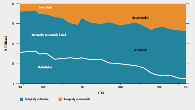
In many cases, our use of wild populations has directly led to their extinction. The history of passenger pigeons (see section 6.1) and great auks (see Table 6.2) are examples. In many more cases, our use has been a contributing factor to extinctions. The extinction of many large North American mammals at the end of the Pleistocene is an example (see section 1.1). We haven’t lost our fondness for large animals. As mentioned earlier, large body size is one of the emerging risk factors for extinction during the Anthropocene. The pattern is particularly notable in vertebrates, where the largest species are suffering disproportionate population declines relative to smaller species. A study that analyzed data from the IUCN Red List found that the single greatest current threat to vertebrate megafauna is from humans harvesting them for food or body parts (Fig. 6.15). Another study estimated that 7% of all assessed terrestrial mammals are threatened with extinction because humans hunt them for food or medicine.87
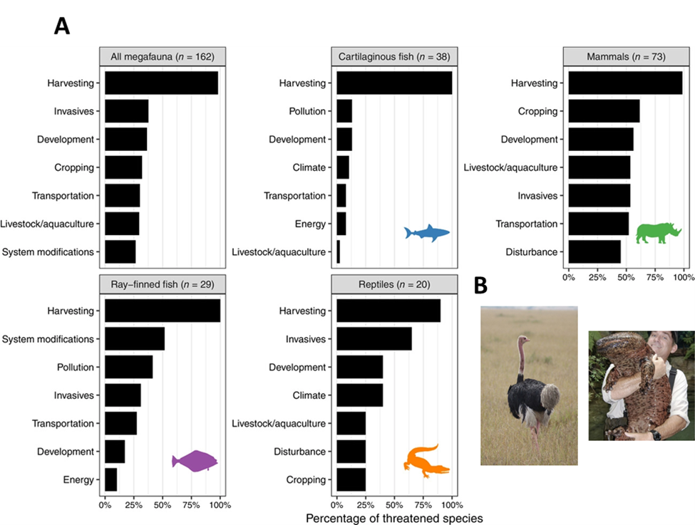
Causes of Overexploitation
It is counterintuitive that the less we depend on wild populations, the more we are affecting them. Indeed, we tend to underestimate our power to drive population numbers down. When the British biologist Thomas Henry Huxley addressed the 1883 International Fisheries Exhibition in London, he opined, “With existing methods of fishing . . . it is inconceivable that the great sea fisheries, such as those for cod, herring and mackerel, could ever be exhausted.”
Huxley didn’t believe we could make any dent to fish numbers in the face of their prodigious biological capacity. That was despite the fact that the conference he was addressing had been convened because of growing fears that fishery stocks around the world were being depleted.88 A little more than 100 years after Huxley’s address, the number of Atlantic cod (Gadus morhua) had dropped so precipitously that Canada halted most of its commercial fishing for it, instantly putting 400,000 people out of work.89 Despite coordinated efforts to apply sophisticated scientific fishery management, cod numbers throughout the Atlantic are still a distant echo of what they once were.90
Our continuing ability to reduce wild populations is related to three main factors.
Technological Advances
As prey get rarer, it gets harder for predators to find them. As a result, predators either decline in numbers themselves or switch to some other more abundant species to eat. That acts as a powerful negative feedback that tends to prevent predators from driving their prey to extinction. In our case, technological advances have progressively lowered the per unit cost of harvesting wild populations, making it viable to continue harvesting even as populations decline. Fisheries provide a good example.
The size of the global fishing fleet doubled between 1950 and 2015. The expanded fleet is also more adept and powerful. That includes industrial-scale vessels equipped with the latest communication, navigation, and fish-finding technologies, as well small vessels owned by individuals. The global fleet is dominated by those smaller vessels, and in 1950, most of them were wind or human powered. By 2015, 68% of the global fishing fleet was motorized.91 These advances have dramatically increased our capacity to catch fish. Framed another way, the intensity of effort that we expend trying to catch fish has more than doubled since 1950. Despite the increasing effort, the global catch of fish plateaued in the 1980s and has declined slightly since. That reflects the fact that fish abundance has been declining, requiring us to work increasingly harder to catch the same amount of fish.
One way that we have compensated for the increasing rarity of species is by adding new species to our fishing list. Technological advances have helped find fish species that used to be too difficult or expensive to exploit. For example, bottom trawling is a common fishing technique that involves dragging a net along the bottom. Up until the 1950s, bottom trawlers could only be deployed in shallow waters, but technological advances allowed bottom trawlers to fish at greater depths. The depletion of shallow water fisheries has provided a powerful incentive to do so. Many deep-sea fishes are particularly vulnerable to overexploitation because they grow slowly, have low reproductive rates, and have limited capacity for population growth.92
Increased Demand
Adding new species to our fishing list usually doesn’t mean that we stop fishing the species we had been overexploiting. We often continue to fish populations even as they become rare. As of 2019, 91 globally threatened marine species were still being fished on an industrial scale.93 The reasons why we still exploit rare species or threatened ecosystems stem from the complex socioeconomic changes that have been occurring during the Anthropocene (see Chap. 1) These changes have kept the demand for wild populations high even as our overall societal dependence on them has decreased.
At a basic level, there are just a lot more of us around, so even if a shrinking proportion of humans exploit wild populations, the absolute magnitude of the impact can still be high. But, as usual, the story is more nuanced than that. At one end of the socioeconomic spectrum, the poorest among us still often depend on wild populations to provide necessities like food, fuel, and medicine. Millions of people around the world depend on wild harvested meat for food. In the most food-insecure countries, wild-harvested meat provides a significant proportion of the animal protein consumed by their citizens. As of 2019, Côte d’Ivoire was in the bottom third of 113 analyzed countries in terms of food security, and its people got 73% of their animal protein from wild meat.94
At the other end of the socioeconomic spectrum, we often still desire wild species even after we become more financially secure and less dependent on wild populations. That is partly because wild species are significant parts of our cultural identity, such as being ingredients in traditional foods and medicines or serving as symbols in cultural and religious ceremonies. The rise of the global middle class and the move from rural areas to cities has driven increasing demand from people who don’t live near wild populations but who have a little extra cash to occasionally buy the ingredients for traditional meals, the materials for ceremonial clothing, or the components of traditional medicines. In many cases, wild-sourced products have a cachet that partly stems from their rarity. They have become luxury items that are used to present status, impress business clients, and celebrate major life events. For example, in Hue, Vietnam, most of the consumers of wild meat are young, educated, and relatively well off financially, and they mostly eat wild meat in restaurants.95
Globalized Markets
The trade in wild animal products is increasingly global and illicit, with a mostly negative effect on how we exploit wild populations. The local users of wild populations have strong incentives to manage the resource sustainability, and they often have the expert knowledge to do so.96 The procurement and distribution networks that develop to supply wild products to far-flung markets often have neither the incentive nor the knowledge to sustainably manage local wild populations. In addition, much of the trade has been driven underground as countries establish bans and restrictions on the trade of wildlife. Criminal gangs typically do not have conservation departments.
Our increasingly connected global culture can also drive demand. Fashions and fads that may have once been restricted to a particular region can now spread globally. The United States has relatively few restrictions on the import or export of reptiles, and it has a large trade in reptile pets (Fig. 6.16). The vibrant US market strongly influences the illicit reptile trade in other parts of the world, such as Australia, where reptile imports are effectively banned. The reptile species that are smuggled into Australia closely mirror those found in the US market. On average, illicit reptile species start showing up in Australia about 5.6 years after they first appear in the United States.97
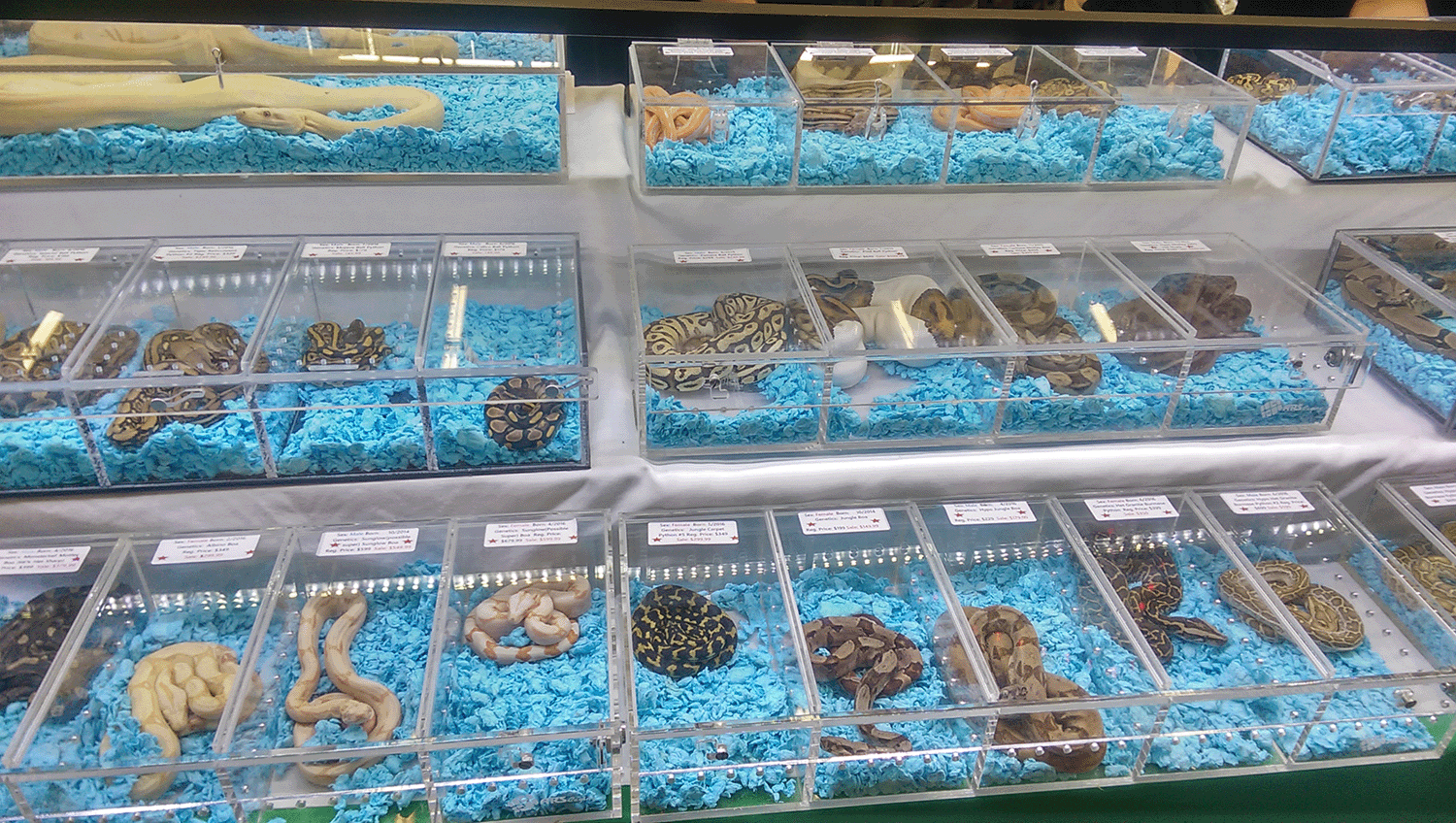
Reorganized Food Webs
One of the more general effects of our exploitation of wild species is that it rearranges food webs and alters the flow of energy and materials through ecosystems. Perhaps the prime example of this effect is how our exploitation of marine species is reorganizing the trophic structure of the ocean. In many parts of the ocean, we appropriate 30% or more of the annual net primary production through our fisheries, and the spatial footprint of that intense use has spread considerably since 1950 (Fig. 6.17).
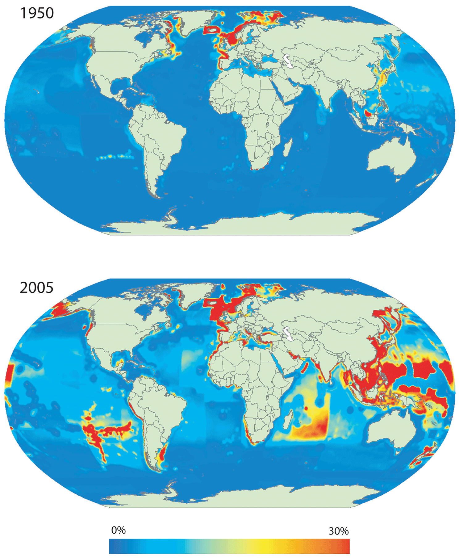
All that biomass appropriation is not simply because we catch a whole lot of biomass (although that’s part of the reason). Keeping with our long-standing predilection for exploiting megafauna, we often make top predator species the targets of our fisheries. Energy transfer between trophic levels in marine food webs is only about 12%.98 As a result, the harvest of top predators such as Atlantic bluefin tuna (Thunnus thynnus) requires considerably more supporting primary production than species at lower trophic levels, such as the filter-feeding northern anchovy (Engraulis mordax). To exacerbate matters, large top predators tend to have lower population growth rates and have less capacity to replace the individuals removed by overfishing compared to smaller species. This has caused dramatic population declines among the species that make up the top trophic levels in marine ecosystems. Sharks are a notable example. In 2021, one-third of Chondrichthyes species (sharks, rays, and chimeras) were threatened with extinction, and three species hadn’t been seen in more than 80 years. In all these cases, overfishing is the primary cause of population decline.99 Many top predators have become increasingly rare and difficult to catch. In the 1960s, long-line fishing for predatory species such as tuna caught an average of 6-12 individuals per 100 hooks set. At the start of the twenty-first century, the same 100 hooks yielded 0.5-2 individuals.100
As our initial fishing targets have become rarer, we have expanded our target list to include species at lower trophic levels, a pattern known as “fishing down” the food web. The fishing history off the coast of Maine is an example.101 Atlantic cod is an apex predator at the top of the western Atlantic marine food web. It had dominated the region’s fishery for thousands of years until its abundance declined precipitously in the 1970s. The commercial fishery then turned to American lobster (Homarus americanus), a predator in the middle of the food web. Herbivores such as sea urchins and sea cucumbers began to be commercially exploited in the 1980s, causing a rapid decline in their local abundance. In the twenty-first century, the fastest-growing part of the fishery has been seaweed and other marine algae. Species at lower trophic levels are inherently more abundant and often more resilient to the effects of our fishing, making them an obvious alternative. Since the 1950s, the mean trophic level of the fish we catch has declined about 0.10 trophic levels per decade.102 Keep in mind that we have expanded our use, not shifted it. For the reasons described above, we have kept fishing top predators even as we expanded our harvests to include species at lower trophic levels. The net result has been a lower overall abundance of marine organisms that are organized into functionally simpler and shorter food webs.103
Even if we exploit relatively few species, the effects can be profound. Dramatic reductions in population abundance caused by our overexploitation can trigger trophic cascades that have ripple effects throughout entire ecosystems. A classic example is what happened as a result of our hunting sea otter (Enhydra lutris). Sea otters are cute and cuddly, but we have a long history of hunting them. Indigenous peoples along the Pacific Coast apparently hunted sea otters in the waters around their settlements, partly to keep them from eating the large mussels that they also prized as a food source.104 In the eighteenth century, we started hunting them on an industrial scale, primarily for their luxuriant fur. By the start of the twentieth century, there were only an estimated couple thousand sea otters left, spread across the coastal waters of eastern Russia and western North America. In California, only about 50 individuals survived the slaughter. The dramatic reduction in the abundance of sea otters triggered a trophic cascade (Fig. 6.18). Besides being cute, sea otters are voracious predators of many invertebrates such as sea urchins (Strongylocentrotus spp.), which in turn are voracious predators of kelp (Order Laminariales). When sea otter numbers crashed, urchin numbers boomed. Large, roving bands of urchins created widespread overgrazed bare patches called urchin barrens.
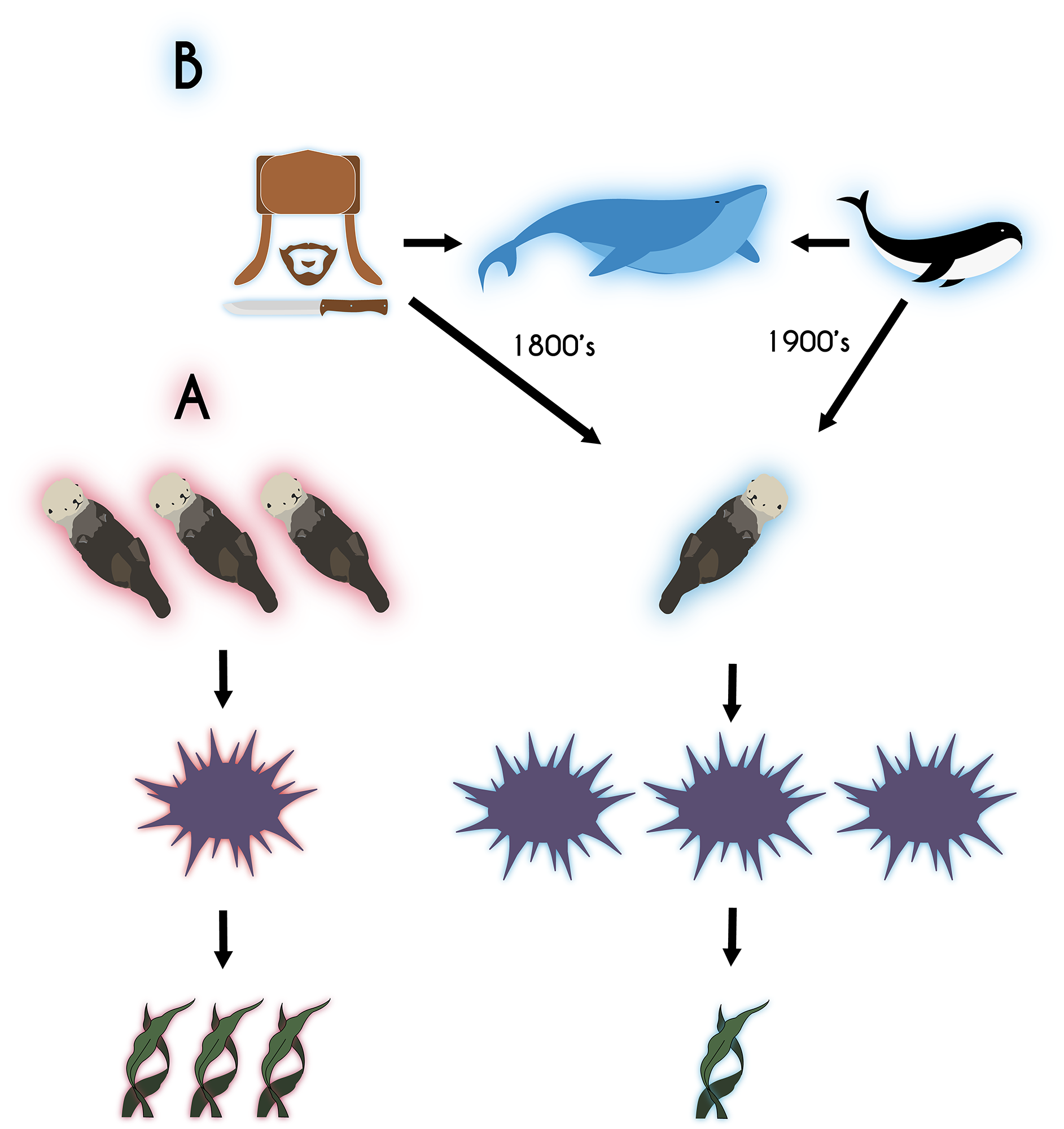
The loss of kelp had significant effects on the entire coastal ecosystem. Far less energy (and carbon) is fixed from photosynthesis in barrens than in kelp forests. The net primary productivity of intact kelp forests is 313–900 g C m–2 yr–1, while that of otter induced barrens is only 25–70 g C m–2 yr–1.105 Consequently, far less energy is available to fuel other parts of the food web. For example, filter-feeding mussels and barnacles have higher growth rates.106 and fish are more abundant.107 in locations where otters maintain stands of kelp. Steller’s sea cow (Hydrodamalis gigas), which as the name suggests ate kelp, likely went extinct as a result of the loss of kelp triggered by the overhunting of sea otters.108 Kelp is also a strong ecosystem engineer that supports the habitat requirements for many other species. For example, the shade from tall kelp suppresses the growth of understory algae species that would otherwise outcompete sessile invertebrates for space on the bottom.109 Even species that are seemingly far removed from kelp are affected by the human-otter-urchin relationship. In British Columbia, bald eagles (Haliaeetus leucocephalus) sometimes build nests using the woody stems of the long-lived kelp (Pterygophora californica) that wash ashore as wrack, but this only happens in areas where otters are present and kelp is abundant.110 Individual bald eagles also dramatically shift their diet depending on whether nearby waters have kelp forests or urchin barrens.111
Things are even more complicated than that. Just before we hunted sea otters nearly to extinction, we initiated a series of remarkably successful conservation efforts. By the early 1980s, sea otter populations had rebounded in many places, and kelp forests began to regrow in barren areas. Then, seemingly all of a sudden, sea otter numbers began to crash again across many parts of the northern Pacific. Even more disquietingly, other marine mammal species, such as harbor seals (Phoca vitulina), northern fur seals (Callorhinus ursinus), and Steller sea lions (Eumetopias jubatus) also experienced precipitous declines at about the same time. It seemed like a new deadly disease was sweeping its way through the North Pacific. We are still not entirely sure what is happening, but we have evidence that one cause might be something deadly that had always been there: orcas (Orcinus orca). Orcas, colloquially known as killer whales, are exquisite predators that through their intelligence and social organization can hunt and kill almost anything. They really like large marine mammals, particularly other whales. But when humans hunted large whales to near extinction after World War II, orcas adjusted their diet. First, they focused more attention on seals and sea lions, and then eventually they even turned their hungry eyes on the tiny bundles of sea otter cuteness.112 In a reprise of the trophic cascade that happened when we directly overhunted sea otters, urchin barrens have reappeared in several places in the North Pacific where orcas have caused declines in sea otters (See Fig. 6.18).113
6.7 Pollution
Section 6.7: Pollution
Overexploitation is perhaps the most direct way that we alter biodiversity patterns: eating a species to extinction is clear-cut. By comparison, pollution is perhaps our most insidious and least understood influence on biodiversity. For one thing, the definition of pollution is broad and fuzzy. One definition is any substance that we add to the environment that harms ourselves or other organisms. That’s a long list of stuff that includes novel materials such as plastic and pesticides as well as natural materials such as nitrogen and lead. A broader definition includes the energy we add to ecosystems in the form of heat, light, and sound. These energy additions can disrupt the lives of organisms just as much as toxic chemicals can.
There is considerable ambiguity about what “harmful to ourselves or other organisms” means in practice. While many pollutants are highly toxic to organisms, many others exist along a fuzzy continuum of toxicity that varies by the type of organism, the age or life stage of the organism, the environmental concentration of the material, where and when organisms are exposed, and a range of other contextual circumstances. Also, organisms are increasingly exposed to complex and constantly changing cocktails of pollutants that potentially interact, creating effects that are difficult to predict based simply on the individual properties of the component pollutants. As a result, the effects that pollutants have on organisms are often subtle, chronic, take a long time to manifest, or vary considerably across space, time, and all the other vagaries of life that organisms encounter.
Still, we have developed a much greater appreciation for the fact that our additions of materials and energy can have a wide range of harmful effects on individual organisms. We are also beginning to more clearly see how those effects translate into changes in broader biodiversity patterns.
Novel Materials
Conceptually at least, one of the clearest ways we have altered the planet is by creating a long list of novel chemical compounds that we have added to the biosphere in often prodigious amounts. We also have many unambiguous cases where we almost poisoned species to extinction with these chemicals. A classic example is the impact that our use of dichlorodiphenyltrichloroethane (DDT) and other chlorinated hydrocarbon pesticides had on wildlife. Sixty-five years after DDT was first synthesized in 1874, Paul Hermann Müller discovered it was remarkably good at killing insects. We quickly used DDT to do just that on a prodigious scale. There was hardly a situation or place where we didn’t use DDT to help manage insect pests (Fig. 6.19). But just a few years after we started to extensively use DDT and similar chemicals as insecticides, we began to notice their environmental downsides. Among other things, they are acutely toxic to a wide range of organisms, not just the few pest species we are targeting. They last a long time in the environment, so their effects linger long after the pest outbreak that caused us to apply the chemical is over. They also bioaccumulate in the tissues of organisms, becoming increasingly concentrated as they move up food webs.

Predatory birds are particularly affected by DDT. The process of metabolizing the high concentrations of chlorinated hydrocarbons in their food disrupts the metabolic pathways that integrates calcium carbonate into eggshells. The resulting malformed eggshells are thin and break easily. Beginning in the 1950s, DDT caused widespread and catastrophic declines to the reproductive output of many top predatory birds such as hawks, falcons, and eagles. Many species were pushed to the brink of extinction, including the bald eagle (Haliaeetus leucocephalus), the iconic symbol of the United States. By 1963, there were only 487 nesting pairs in the lower 48 states.114 We quickly accumulated a large body of evidence that unambiguously linked the population declines to our use of DDT and similar chemicals.115 The strength of the scientific evidence raised our awareness about the risks of chemical pesticides, and it helped to spur a broader reevaluation of how we use them. DDT was banned in the United States in 1972, and many bird species, including bald eagles, have since made a dramatic recovery.116
But the clear-cut harm caused by DDT and the unambiguous success story we had in identifying and mitigating those harms represent an exceptional case. We have a far less complete understanding of the biological effects of most of the novel chemicals we are creating. Earth is now awash with novel chemicals whose impact on organisms is essentially unknown. One difficulty we have is that the biological effects of many chemicals are far more subtle or involve more complex pathways and interactions than the effects of DDT. In addition, organisms are now chronically exposed throughout their entire lives to mixtures of multiple chemicals at low doses. We have growing evidence that long-term chronic exposure and the synergistic effects of different chemicals can have profound cumulative effects on individuals and populations.
An example of this growing understanding involves the neonicotinoid class of pesticides. Neonicotinoids were developed and marketed in part because they are less directly toxic to vertebrates. If you have a cat or dog, you have probably given them a neonicotinoid to control their fleas and ticks. As comparatively benign as they are to vertebrates, neonicotinoids are decidedly toxic to a broad range of insects. In addition, they have the neat property of being moderately long lived (over the span of months) and can be absorbed by plant tissues. This allows farmers to make a few applications that inoculate crops against a wide range of insect pests for relatively long windows of time. A common application approach is to coat seeds with neonicotinoids, which bestows insect resistance to the young growing crops. Such advantages have made neonicotinoids popular, but this popularity has created some potential problems. Traces of neonicotinoids are now ubiquitous in the soil, water, and the tissues of organisms around the world.117 This ubiquity stems more from our constant and prodigious use of them than it does from there moderate persistence in the environment. As a result, most organisms living in or near our domesticated landscapes are now chronically exposed. There is emerging evidence that this chronic exposure effects organisms that aren’t the targets of our neonicotinoid use or acutely sensitive to the exposure. These include zooplankton,118 birds,119 fish,120 and ourselves.121
In most of these cases, the effects are subtle, and we still don’t fully understand what the consequences will be.
Ruby-throated hummingbirds (Archilocus colubris) rapidly metabolize neonicotinoids they are exposed to. That metabolism comes at a steep energetic cost, however, and it is not clear how the added cost affects things like foraging behavior, migration, or breeding success.122 But we are beginning to get more detailed data. In one wonderfully designed experiment, researchers captured migrating white-crowned sparrows (Zonotrichia leucophrys) and exposed them to a common neonicotinoid pesticide at doses the birds commonly encounter in the wild. White-crowned sparrows are seed eaters, so they often consume neonicotinoid coated seeds. The researchers then let the pesticide-exposed birds free to get on with their migration, but only after attaching a small nanotag that allowed the researchers to track the birds. After their release, the pesticide-exposed birds ate considerably less food and put on less body mass and fat than non-exposed birds, who also had been given a nanotag. As a result, the pesticide-exposed birds delayed leaving on the next leg of their migration, likely to regain fuel stores and recover from the intoxication. Pesticide-exposed birds stayed at the release site a median of 3.5 days longer than non-exposed control birds.123
Most of the research that has so far been done to understand the effects of chronic neonicotinoid exposure has involved the insects inhabiting or passing through agricultural landscapes. These include a range of non-pest insects that provide us with critical ecosystem services such as pollination. Pollinators appear to get particularly high exposures because they can take up neonicotinoids via the pollen and nectar of treated crops or nearby non-crop plants that take up the chemicals from contaminated water. But the level of this incidental exposure is typically well below levels that cause death. Until recently, we had almost no idea what impacts—if any—those chronic low doses had on organisms.
The data we are now getting from comprehensive field studies suggest the answers are not simple. From the data we have, it appears that a range of wild bee species as well as managed honeybees are harmed by their real-world exposure to neonicotinoids. The level of that harm depends on the specific environmental conditions and circumstances in which that exposure takes place, however. In one study, researchers placed three bee species (honeybees and two wild species) in oilseed rape fields that were either treated with neonicotinoids or not. They then followed the bees over a couple of years, tracking their exposure levels and evaluating their demographic performance across 33 sites in three countries (Hungary, Germany, and the United Kingdom). In Hungary and the United Kingdom, bees that lived near and foraged in neonicotinoid treated crops had reduced reproductive output and smaller colony sizes relative to bees that foraged in non-neonicotinoid-treated fields. In Germany, however, bees were largely unaffected by neonicotinoid treatments, and in fact the colony size of honeybees was greater in the neonicotinoid treated fields. The difference in Germany may be that bees there have access to a more diverse diet in the form of diverse flower borders and hedgerows. As a result, German bees might be healthier overall compared to bees in the United Kingdom and Hungary that have a more monotonous less nutritious diet, and that may help them better handle the stress of neonicotinoid exposure.124 The effects that neonicotinoids have on bees are also influenced by all the other chemicals that bees are exposed to. For example, one study found that the negative effects of neonicotinoid exposure were significantly enhanced when bees were also exposed to commonly encountered levels of fungicides.125
We have evidence from a range of other organisms and systems that pollutants frequently interact with each other and other stressors to produce complex and variable impacts on organisms. Tree swallows (Tachycineta bicolor) living in areas contaminated with high levels of mercury suffer significantly reduced reproductive success compared with tree swallows living in less contaminated areas. The impact of mercury depends on the weather, however. The negative effects of mercury are much more pronounced if conditions are abnormally warm during the early part of the nesting period. It is unclear why, but young, featherless birds are particularly vulnerable to temperature fluctuations, and any behavioral or physiological impairment caused by mercury seems to have an elevated impact during this critical time.126 We can hypothesize that if the frequency or magnitude of springtime warm spells increased as a result of climate change, swallows that lived in mercury-contaminated areas would be negatively affected even if the individual levels of warming or mercury exposure did not cause harm on their own.
The biological effects of novel chemicals can also ripple through ecosystems and affect broad biodiversity patterns, not just the few species that are acutely sensitive to the chemicals. For instance, there is correlative evidence that the prevalence of neonicotinoids has been a contributing factor in ongoing declines in the abundance and species diversity of birds across North America, with grassland and insectivorous birds being particularly affected.127 Neonicotinoids can directly affect the physiology of some bird species, but much of their impact on birds probably occurs indirectly through their effects on the abundance and biodiversity of the insects that birds feed on.
Excessive Amounts of Natural Materials
It is not just novel chemicals that are pollutants. As I describe in Chapter 3, one of the main ways that we have changed ecosystems is by augmenting the flow of natural materials. While these additions are rarely acutely toxic to organisms, they have a range of indirect effects that in many cases completely transform biodiversity patterns. For example, we have more than doubled the amount of reactive nitrogen flowing through Earth’s ecosystems (see Fig. 3.11), with a profound impact on global biodiversity patterns. Although there are some exceptions and contextual complexities, the added nitrogen has by and large reduced biodiversity. The primary way this happens is that some species are better equipped to use the excess nitrogen than others. These species can better channel the nitrogen into more and quicker growth, giving them a competitive advantage. The competitively advantaged species tend to crowd out other species and become numerically dominant, which in turn tends to reduce species and functional diversity. This is what appears to be happening in many terrestrial plant communities that are exposed to elevated nitrogen.
A meta-analysis of long-term experiments conducted in herbaceous plant communities around the world estimated that elevated nitrogen reduces species richness by an average of 16%.128 Which species benefit from the added nitrogen varies across communities and ecosystems, but one functional group that tends to be a frequent winner is grass.129 Grasses are particularly adept at converting excess nitrogen into prodigious amounts of above- and belowground biomass. The prodigious biomass can directly crowd out other species, but it can also influence biodiversity through a range of indirect effects like increasing the frequency and timing of wildfire and altering soil conditions. In the southwestern United States, nitrogen in the form of air pollution from big cities like Los Angeles has fertilized large swaths of the landscape. The added nitrogen has contributed to the spread and increased abundance of naturalized non-native grass species such as buffelgrass (Pennisetum ciliare) (see Fig. 9.4). In some places, the grasses have directly crowded out annual forbs that contribute to beautiful spring wildflower displays. In other places, the increased fuel provided by the fertilized grasses has increased fire intensity and frequency, which in turn has reduced shrub cover and favored the grasses even more.130
An illustration of the strong influence nitrogen can have on patterns of plant diversity comes from an over 160-year-old experiment called Park Grass located at the Rothamsted Experimental Station in the United Kingdom. Beginning in 1856, researchers applied a series of fertilizer treatments to a swath of pasture and have been following what happened to the plants ever since. Plots that have been fertilized with nitrogen have significantly fewer species than unfertilized plots. Instead of the diverse mixture of species and functional types seen in the unfertilized plots, fertilized plots are dominated by grasses, have fewer forbs, and have almost no nitrogen-fixing species. The researchers could not control every environmental aspect in their experiment. Most annoyingly for them was the fact that all the plots received a significant amount of nitrogen from air pollution. This had the effect of elevating nitrogen in all the plots, even in the controls that received no experimental additions of nitrogen. That complicated the analysis of their results a bit, but it also helped to illustrate the significant effect that nitrogen availability had on diversity patterns.
Since about 1985, the level of airborne nitrogen pollution has been steadily decreasing as a result of pollution control measures. The species composition and diversity of the Park Grass plots have responded to the reduced nitrogen. Over the past few decades, species richness, species diversity, and the proportion of nitrogen fixers increased across all the plots, even in the experimentally fertilized ones.131 A similar pattern has been observed for all the plant species across Britain. Great Britain has particularly detailed and long-term records of plant species richness. A statistical analysis of these records suggests that between 1800 and the late twentieth century, the combination of nitrogen and sulfur deposition from air pollution decreased local plant species richness by an average of 39% across Britain. But local species richness has started to recover in recent decades as a result of air pollution mitigation efforts.132
Nitrogen pollution has arguably had an even bigger impact on diversity patterns in aquatic systems. Eutrophication is the gradual increase of nutrients in aquatic habitats. Many aquatic habitats, particularly those in the ocean, have naturally low levels of reactive nitrogen, and the organisms that live there are hypersensitive to any increases in its availability. In these nitrogen-limited habitats, even modest inputs of nitrogen pollution can kick primary production into overdrive. Like in terrestrial environments, some species of primary producers benefit from fertilization more than others. For instance, eutrophication-driven blooms in phytoplankton tend to be dominated by a few species of cyanobacteria.133 These blooms of a few species can lower the abundance or diversity of other primary producers, which can in turn have a cascade of effects throughout the rest of the ecosystem. For example, in shallow coastal habitats, nitrogen pollution feeds the growth of epiphytic algae that can smother seagrass beds. Seagrasses are strong ecosystem engineers, and their decline can cause a shift to an entirely algae-dominated system that is typically less diverse in terms of animal species and supports diminished ecosystem services such as fish habitat.134
Another indirect impact of nitrogen pollution in aquatic systems is anoxia. The pace of primary production and its recycling tends to go much faster in water than on land, where a lot of the primary production gets hung up for long periods in the form of woody biomass or soil carbon. In aquatic environments where much of the primary production is done by single-celled organisms or soft-bodied algae, most biomass decomposes as quickly as it is created. Booms in biomass production invariably lead to booms in decomposition, which can locally consume much of the available oxygen. Pollution-driven hypoxic dead zones have proliferated in coastal waters around the world. Coastal hypoxic zones are often seasonal, reflecting natural cycles of runoff and phytoplankton growth in temperate regions. One of the largest hypoxic zones in the world forms every year in the northern Gulf of Mexico. Nutrient-laden spring runoff from the Mississippi and Atchafalaya Rivers feeds a phytoplankton boom that eventually ends in an oxygen-sapping decomposition bust by midsummer (Fig. 6.20). The amount of nitrogen flowing into the northern Gulf of Mexico at the start of the twenty-first century was more than double the amount flowing in at the start of the twentieth century, and that has increased the size, frequency, and seasonal duration of the hypoxic zone.135 Globally, coastal hypoxic zones have been spreading exponentially since the 1960s, also largely as a result of increased nutrient levels in coastal waters.136
As you might expect, hypoxia is not terribly good for the animals living there, and befitting their colloquial name, hypoxic zones regularly kill marine organisms, stress them, or force them to move. But there is a lot of variability in both the strength and duration of the hypoxic periods as well as how organisms respond to hypoxia. In fact, in some cases, moderate levels of eutrophication can increase the overall productivity of ecosystems by moderately increasing primary production without causing much damaging hypoxia. But overall, strong and prolonged periods of hypoxia tend to reduce local diversity and diminish key ecosystem services such as fisheries. The most severe hypoxic zones produce markedly less secondary biomass (i.e., fish) than do regions that don’t experience hypoxia. The scale of this pollution-caused missing biomass is impressive. In some of the world’s worst hypoxic zones that form in the Baltic Sea, hypoxia reduces secondary production by a staggering 30%.137
Additions of Energy
One of the main ways that we alter the flow of materials and energy through ecosystems is through the structures that we create, that is, physical ecosystem engineering (see section 3.5). Altering the flow of energy may sound a little abstract, but it is one of the important ways that we modify habitat conditions for organisms. Prime examples are the unique patterns of heat, sound, and light that characterize our urban environments (see Fig. 3.16). Organisms are affected by these new conditions in a wide variety of ways. I describe some of these in more detail in Chapter 8
In some respects, these urbanized conditions fall under the category of ecosystem domestication. But in other respects, it’s handy to view the changes to energy flows as a form of pollution. Changes in light, sound, and temperature can negatively affect organisms in much the same way that being exposed to chemical pollutants can. For example, the water flowing through many temperate streams tends to be cool even during the summer. Many of the aquatic organisms in these streams are physiologically stressed if it gets even modestly warm. For instance, several salmon species (Salmonidae) are physiologically stressed if stream temperature goes above 18°C, and they begin to die if it reaches 21°C.138 We have been increasing the temperature of cool water streams through land use change, the injection of warm water from industrial processes, and climate change. In the Pacific Northwest, thermal pollution is a significant reason why salmon populations are in precipitous decline, and several are on the brink of extinction.139
6.8 About Those Interactions
Section 6.8: About Those Interactions
When I started describing the forces driving biodiversity change, I mentioned that they commonly interact. I then promptly decided that I didn’t want to deal with all those complications. But we really should consider them, if only briefly. The main forces I describe above don’t act in isolation; it is their combined and often interacting influence that is driving biodiversity change and contributing to the sixth extinction.
The combination of factors that are contributing to the decline of coral reefs provide an example. As I describe in Chapter 3, tropical coral reefs are teaming with herbivorous fish. These fish depress the abundance of turf-like macroalgae that would otherwise compete with the coral for space and with the coral’s symbiotic zooxanthellae for light. These fish have been severely overexploited on many reefs, both for food and for the aquarium pet trade. Herbivorous fish in the tropical Atlantic have also suffered from the introduction of predatory Pacific red lionfish (Pterois volitans). Lionfish, which ironically were likely introduced to the Atlantic from aquariums, have novel hunting strategies that Atlantic fish are not well prepared to deal with.140 Overfishing and the effects of lionfish have given macroalgae a competitive edge over corals and triggered dramatic shifts from coral to algae-dominated communities in some locations (see Fig. 3.2).
By themselves, those stressors are not enough to explain the precipitous global decline in coral reefs. Since the 1950s, many coastal tropical waters have become enriched with nitrogen and phosphorous, primarily as a result of polluted runoff from domesticated ecosystems in the adjacent terrestrial landscape. The nutrients have given the algae a decided competitive edge over coral, even in the presence of abundant herbivorous fish.141 Corals are resilient and in many locations can still nevertheless hold their own against the turbocharged algae. But the effort is exhausting and uses energy that otherwise could go to support a range of other physiological and life history processes that buffer corals from all the other stresses and vagaries of life. The intensity and variety of those stresses have been steadily increasing.
Periods of excessively warm water as well as lowered pH physiologically stress coral, and the frequency and intensity of both have been increasing with increasing atmospheric CO2 (see Chap. 5). A range of novel chemical pollutants also likely stress corals in ways that we still don’t fully understand. For instance, the ingredients of many sunscreens have been shown to negatively affect the health of corals as well as that of many reef-dwelling organisms.142 The long list of stresses directly and indirectly alter the microbiome-inhabiting coral organisms (see Fig. 5.8), which in turn makes the corals much more susceptible to pathogens and disease.143
Stressed-out and sickly coral is less able to recover from the periodic disturbances that corals have always dealt with. Things like big storms that physically wash out chunks of the reef or periodic outbreaks of coral predators such as the crown-of-thorns seastar (Acanthaster planci). In the past, such disturbances were inconsequential blips in the vast and robust coral ecosystems of the planet. Now, they are increasingly the coup de grâce at the end of a long, complex chain of decline. All together, the combined effects of these stressors have caused the global coverage of living coral to decline by half since the 1950s.144
Chapter Summary
Brave New World
We are rapidly changing and reorganizing biodiversity to an extent that is on par with the five previous periods of profound change in the history life. We are doing this by causing climate change, domesticating ecosystems, moving organisms, exploiting organisms, and causing pollution.
- We are experiencing a rapid reduction in the abundance of some organisms and the extinction of species. The pace of the extinctions is similar to that observed in Earth’s five previous major extinction events (Tables 6.1, 6.2, Figures 6.2, 6.3)
- Species most at risk of extinction are those that have specialized requirements, restricted ranges, relatively large body size, and low reproductive rate (Figure 6.4).
- Biodiversity is declining at the global scale while both increasing and decreasing at smaller spatial scales (Table 6.3). Novel associations of biodiversity are forming, and old associations are being lost (Figures 6.1, 6.13). Biodiversity is tending to become more homogenous across space (Figures 6.7, 6.12). The pace of change is increasing (Figures 6.2, 6.5)
- The pace of climate change will likely be too quick for some species to adapt to behaviorally, physiologically, or evolutionarily. The climate driven movement of organisms will also create new associations of species and new interactions among species that will change ecosystem function and services
- The conversion of diverse habitats into domesticated ecosystems is a significant cause of biodiversity loss (Figure 6.6). But some forms of domestication can maintain or even increase biodiversity—at least for some metrics and at intermediate spatial scales (Figures 6.7A, 6.8)
- Our breeding of organisms creates new genetic forms and phenotypes (Figure 6.9), but it also tends to be a strong filter that reduces overall levels of genetic and phenotypic diversity.
- Our movement of species tends to increase species richness at local and regional scales but decrease the uniqueness of species among locales and regions. The movement also creates novel species interactions that can reduce local and regional diversity (Figure 6.11) and homogenize the functional diversity of ecosystems (Figures 6.12, 6.13)
- Our exploitation of wild species has intensified and is a significant cause of biodiversity loss (Figures 6.14, 6.15, 6.16). Exploitation causes population declines both directly and indirectly and also reorganizes species relationships in ecosystems (Figures 6.17, 6.18)
- Pollution is another significant driver of biodiversity change. The effects of some pollutants are strong, direct, and well understood (Figures 6.17, 6.18), but the effects of many others are chronic, subtle, and not well understood.
Additional Resources
- International Union for the Conservation of Nature (IUCN) Red List of Threatened Species. Although far from comprehensive, this is the most extensive database we have of the ecological status of the world’s species. It is an important resource for governments, communities, and conservation organizations: http://www.iucnredlist.org/
- Last Chance to See, by Douglas Adams and Mark Carwardine (New York: Harmony Books, 1990). The authors travel to see nine species that were then on the brink of extinction. The book was also adapted into a BBC documentary in 2009: https://www.bbc.co.uk/programmes/b00vxzcj
- The Sixth Extinction: An Unnatural History, by Elizabeth Kolbert (New York: Henry Holt, 2014). This book offers a comprehensive exploration of how we are creating a mass extinction event.
- Cane Toads: An Unnatural History, by Mark Lewis. A classic documentary about one particularly interesting invasive species: http://naturedocumentaries.org/7168/cane-toads-unnatural-history-mark-lewis-1988/
References
19Allred, B.W., Fuhlendorf, S.D., Hamilton, R.G., 2011. The role of herbivores in Great Plains conservation: comparative ecology of bison and cattle. Ecosphere 2, art26. https://doi.org/10.1890/ES10-00152.1
*Alstad, A.O., Damschen, E.I., Givnish, T.J., Harrington, J.A., Leach, M.K., Rogers, D.A., Waller, D.M., 2016. The pace of plant community change is accelerating in remnant prairies. Sci. Adv. 2, e1500975. https://doi.org/10.1126/sciadv.1500975
81Anderson, C.B., Vanessa Lencinas, M., Wallem, P.K., Valenzuela, A.E.J., Simanonok, M.P., Martínez Pastur, G., 2014. Engineering by an invasive species alters landscape-level ecosystem function, but does not affect biodiversity in freshwater systems. Diversity Distrib. 20, 214–22. https://doi.org/10.1111/ddi.12147
111Anthony, R.G., Estes, J.A., Ricca, M.A., Miles, A.K., Forsman, E.D., 2008. Bald eagles and sea otters in the Aleutian Archipelago: indirect effects of trophic cascades. Ecology 89, 2725–35. https://doi.org/10.1890/07-1818.1
78Ayres, D.R., Strong, D.R., Baye, P., 2003. Spartina Foliosa (Poaceae)—a common species on the road to rarity? Madroño 50, 209–13.
38Baccini, A., Walker, W., Carvalho, L., Farina, M., Sulla-Menashe, D., Houghton, R.A., 2017. Tropical forests are a net carbon source based on aboveground measurements of gain and loss. Science 358, 230–34. https://doi.org/10.1126/science.aam5962
91Bell, J.D., Watson, R.A., Ye, Y., 2017. Global fishing capacity and fishing effort from 1950 to 2012. Fish Fish. 18, 489–505. https://doi.org/10.1111/faf.12187
31Belliard, J., Beslagic, S., Boucault, J., Zahm, A., 2021. Increasing establishment of non-native fish species in the Seine River basin: insights from medium- and long-term approaches. Front. Ecol. Evol. 9, 528. https://doi.org/10.3389/fevo.2021.687451
75Bergström, A., Stringer, C., Hajdinjak, M., Scerri, E.M.L., Skoglund, P., 2021. Origins of modern human ancestry. Nature 590, 229–37. https://doi.org/10.1038/s41586-021-03244-5
35Blowes, S.A., Supp, S.R., Antão, L.H., Bates, A., Bruelheide, H., Chase, J.M., Moyes, F., Magurran, A., McGill, B., Myers-Smith, I.H., Winter, M., Bjorkman, A.D., Bowler, D.E., Byrnes, J.E.K., Gonzalez, A., Hines, J., Isbell, F., Jones, H.P., Navarro, L.M., Thompson, P.L., Vellend, M., Waldock, C., Dornelas, M., 2019. The geography of biodiversity change in marine and terrestrial assemblages. Science 366, 339-45. https://doi.org/10.1126/science.aaw1620
94Booth, H., Clark, M., Milner-Gulland, E.J., Amponsah-Mensah, K., Antunes, A.P., Brittain, S., Castilho, L.C., Campos-Silva, J.V., de Constantino, P.A.L., Li, Y., Mandoloma, L., Nneji, L.M., Iponga, D.M., Moyo, B., McNamara, J., Rakotonarivo, O.S., Shi, J., Tagne, C.T.K., van Velden, J., Williams, D.R., 2021. Investigating the risks of removing wild meat from global food systems. Curr. Biol. 31, 1788-97.e3. https://doi.org/10.1016/j.cub.2021.01.079
4Brockway, L.H., 1979. science and colonial expansion: the role of the British Royal Botanic Gardens. Am. Ethnol. 6, 449–65. https://doi.org/10.1525/ae.1979.6.3.02a00030
96Brondízio, E.S., Aumeeruddy-Thomas, Y., Bates, P., Carino, J., Fernández-Llamazares, Á., Ferrari, M.F., Galvin, K., Reyes-García, V., McElwee, P., Molnár, Z., Samakov, A., Shrestha, U.B., 2021. Locally based, regionally manifested, and globally relevant: indigenous and local knowledge, values, and practices for nature. Annu. Rev. Environ. Resour. 46, 481–509. https://doi.org/10.1146/annurev-environ-012220-012127
130Brooks, M.L., Brown, C.S., Chambers, J.C., D’Antonio, C.M., Keeley, J.E., Belnap, J., 2016. Exotic annual bromus invasions: comparisons among species and ecoregions in the western United States. In: Exotic Brome-Grasses in Arid and Semiarid Ecosystems of the Western US. Springer Series on Environmental Management. Cham, Switzerland: Springer, 11–60. https://doi.org/10.1007/978-3-319-24930-8_2
134Burkholder, J.M., Tomasko, D.A., Touchette, B.W., 2007. Seagrasses and eutrophication. J. Exp. Mar. Biol. Ecol. 350, 46–72. https://doi.org/10.1016/j.jembe.2007.06.024
23Button, D.J., Lloyd, G.T., Ezcurra, M.D., Butler, R.J., 2017. Mass extinctions drove increased global faunal cosmopolitanism on the supercontinent Pangaea. Nat. Commun. 8. https://doi.org/10.1038/s41467-017-00827-7
65Callaway, R.M., Ridenour, W.M., 2004. Novel weapons: invasive success and the evolution of increased competitive ability. Front. Ecol. Environ. 2, 436–43. https://doi.org/10.1890/1540-9295(2004)002[0436:NWISAT]2.0.CO;2
115Carson, R., 1962. Silent Spring. Cambridge, MA: Houghton Mifflin.
9Ceballos, G., Ehrlich, P.R., Barnosky, A.D., García, A., Pringle, R.M., Palmer, T.M., 2015. Accelerated modern human–induced species losses: entering the sixth mass extinction. Sci. Adv. 1, e1400253. https://doi.org/10.1126/sciadv.1400253
579Ceballos, G., Ehrlich, P.R., Dirzo, R., 2017. Biological annihilation via the ongoing sixth mass extinction signaled by vertebrate population losses and declines. Proc. Natl. Acad. Sci. 114, E6089–E6096. https://doi.org/10.1073/pnas.1704949114
24Clavel, J., Julliard, R., Devictor, V., 2011. Worldwide decline of specialist species: toward a global functional homogenization? Front. Ecol. Environ. 9, 222–28. https://doi.org/10.1890/080216
51Comas , I., Coscolla, M., Luo, T., Borrell, S., Holt, K. E., Kato-Maeda, M., Parkhill, J., Malla, B., Berg, S., Thwaites, G., Yeboah-Manu, D., Bothamley, G., Mei, J., Wei, L., Bentley, S., Harris, S. R., Niemann, S., Diel, R., Aseffa, A., … Gagneux, S. (2013). Out-of-Africa migration and Neolithic coexpansion of Mycobacterium tuberculosis with modern humans. Nature Genetics, 45(10), ng.2744. https://doi.org/10.1038/ng.2744
36Comte, L., Olden, J.D., Tedesco, P.A., Ruhi, A., Giam, X., 2021. Climate and land-use changes interact to drive long-term reorganization of riverine fish communities globally. Proc. Natl. Acad. Sci. 118. https://doi.org/10.1073/pnas.2011639118
86Costello, C., Ovando, D., Clavelle, T., Strauss, C.K., Hilborn, R., Melnychuk, M.C., Branch, T.A., Gaines, S.D., Szuwalski, C.S., Cabral, R.B., Rader, D.N., Leland, A., 2016. Global fishery prospects under contrasting management regimes. Proc. Natl. Acad. Sci. 113, 5125–29. https://doi.org/10.1073/pnas.1520420113
84Costello, C., Cao, L., Gelcich, S., Cisneros-Mata, M.Á., Free, C.M., Froehlich, H.E., Golden, C.D., Ishimura, G., Maier, J., Macadam-Somer, I., Mangin, T., Melnychuk, M.C., Miyahara, M., de Moor, C.L., Naylor, R., Nøstbakken, L., Ojea, E., O’Reilly, E., Parma, A.M., Plantinga, A.J., Thilsted, S.H., Lubchenco, J., 2020. The future of food from the sea. Nature 588, 95–100. https://doi.org/10.1038/s41586-020-2616-y
3Crosby, A.W., 2015. Ecological Imperialism. Cambridge: Cambridge University Press.
68Davis, M.A., Grime, J.P., Thompson, K., 2000. Fluctuating resources in plant communities: a general theory of invasibility. J. Ecol. 88, 528–34. https://doi.org/10.1046/j.1365-2745.2000.00473.x
137Diaz, R.J., Rosenberg, R., 2008. Spreading dead zones and consequences for marine ecosystems. Science 321, 926–29. https://doi.org/10.1126/science.1156401
27Dirzo, R., Young, H.S., Galetti, M., Ceballos, G., Isaac, N.J.B., Collen, B., 2014. Defaunation in the Anthropocene. Science 345, 401–6. https://doi.org/10.1126/science.1251817
32Dornelas, M., Gotelli, N.J., McGill, B., Shimadzu, H., Moyes, F., Sievers, C., Magurran, A.E., 2014. Assemblage time series reveal biodiversity change but not systematic loss. Science 344, 296–99. https://doi.org/10.1126/science.1248484
22Doubleday, Z.A., Prowse, T.A.A., Arkhipkin, A., Pierce, G.J., Semmens, J., Steer, M., Leporati, S.C., Lourenço, S., Quetglas, A., Sauer, W., Gillanders, B.M., 2016. Global proliferation of cephalopods. Curr. Biol. 26, R406–R407. https://doi.org/10.1016/j.cub.2016.04.002
142Downs, C.A., Kramarsky-Winter, E., Segal, R., Fauth, J., Knutson, S., Bronstein, O., Ciner, F.R., Jeger, R., Lichtenfeld, Y., Woodley, C.M., Pennington, P., Cadenas, K., Kushmaro, A., Loya, Y., 2016. Toxicopathological effects of the sunscreen UV filter, oxybenzone (benzophenone-3), on coral planulae and cultured primary cells and its environmental contamination in Hawaii and the U.S. Virgin Islands. Arch. Environ. Contam. Toxicol. 70, 265–88. https://doi.org/10.1007/s00244-015-0227-7
106Duggins, D.O., Simenstad, C.A., Estes, J.A., 1989. Magnification of secondary production by kelp detritus in coastal marine ecosystems. Science 245, 170–73. https://doi.org/10.1126/science.245.4914.170
99Dulvy, N.K., Pacoureau, N., Rigby, C.L., Pollom, R.A., Jabado, R.W., Ebert, D.A., Finucci, B., Pollock, C.M., Cheok, J., Derrick, D.H., Herman, K.B., Sherman, C.S., VanderWright, W.J., Lawson, J.M., Walls, R.H.L., Carlson, J.K., Charvet, P., Bineesh, K.K., Fernando, D., Ralph, G.M., Matsushiba, J.H., Hilton-Taylor, C., Fordham, S.V., Simpfendorfer, C.A., 2021. Overfishing drives over one-third of all sharks and rays toward a global extinction crisis. Curr. Biol. 31, 4773-87. e8. https://doi.org/10.1016/j.cub.2021.08.062
62Dyer, E.E., Cassey, P., Redding, D.W., Collen, B., Franks, V., Gaston, K.J., Jones, K.E., Kark, S., Orme, C.D.L., Blackburn, T.M., 2017. The global distribution and drivers of alien bird species richness. PLoS Biol. 15, e2000942. https://doi.org/10.1371/journal.pbio.2000942
144Eddy, T.D., Lam, V.W.Y., Reygondeau, G., Cisneros-Montemayor, A.M., Greer, K., Palomares, M.L.D., Bruno, J.F., Ota, Y., Cheung, W.W.L., 2021. Global decline in capacity of coral reefs to provide ecosystem services. One Earth 4, 1278–85. https://doi.org/10.1016/j.oneear.2021.08.016
119123Eng, M.L., Stutchbury, B.J.M., Morrissey, C.A., 2019. A neonicotinoid insecticide reduces fueling and delays migration in songbirds. Science 365, 1177-80. https://doi.org/10.1126/science.aaw9419
122English, S.G., Sandoval-Herrera, N.I., Bishop, C.A., Cartwright, M., Maisonneuve, F., Elliott, J.E., Welch, K.C., 2021. Neonicotinoid pesticides exert metabolic effects on avian pollinators. Sci. Rep. 11, 2914. https://doi.org/10.1038/s41598-021-82470-3
113Estes, J.A., Tinker, M.T., Williams, T.M., Doak, D.F., 1998. Killer whale predation on sea otters linking oceanic and nearshore ecosystems. Science 282, 473–76. https://doi.org/10.1126/science.282.5388.473
108Estes, J.A., Burdin, A., Doak, D.F., 2016. Sea otters, kelp forests, and the extinction of Steller’s sea cow. Proc. Natl. Acad. Sci. 113, 880–85. https://doi.org/10.1073/pnas.1502552112
129Field, C.D., Dise, N.B., Payne, R.J., Britton, A.J., Emmett, B.A., Helliwell, R.C., Hughes, S., Jones, L., Lees, S., Leake, J.R., Leith, I.D., Phoenix, G.K., Power, S.A., Sheppard, L.J., Southon, G.E., Stevens, C.J., Caporn, S.J.M., 2014. The role of nitrogen deposition in widespread plant community change across semi-natural habitats. Ecosystems 17, 864–77. https://doi.org/10.1007/s10021-014-9765-5
*85Food and Agriculture Organization of the United Nations, 2020. The State of World Fisheries and Aquaculture 2020. Rome: Food and Agriculture Organization of the United Nations.
47Ford-Lloyd, B.V., Schmidt, M., Armstrong, S.J., Barazani, O., Engels, J., Hadas, R., Hammer, K., Kell, S.P., Kang, D., Khoshbakht, K., Li, Y., Long, C., Lu, B.-R., Ma, K., Nguyen, V.T., Qiu, L., Ge, S., Wei, W., Zhang, Z., Maxted, N., 2011. Crop wild relatives—undervalued, underutilized and under threat? BioScience 61, 559–65. https://doi.org/10.1525/bio.2011.61.7.10
69Fricke, E.C., Svenning, J.-C., 2020. Accelerating homogenization of the global plant–frugivore meta-network. Nature 585, 74–78. https://doi.org/10.1038/s41586-020-2640-y
67Fritts, T.H., Rodda, G.H., 1998. The role of introduced species in the degradation of island ecosystems: a case history of Guam. Annu. Rev. Ecol. Syst. 29, 113–40. https://doi.org/10.1146/annurev.ecolsys.29.1.113
80Gribben, P.E., Byers, J.E., Wright, J.T., Glasby, T.M., 2013. Positive versus negative effects of an invasive ecosystem engineer on different components of a marine ecosystem. Oikos 122, 816–24. https://doi.org/10.1111/j.1600-0706.2012.20868.x
73Grosholz, E.D., 2005. Recent biological invasion may hasten invasional meltdown by accelerating historical introductions. Proc. Natl. Acad. Sci. U.S.A. 102, 1088–91. https://doi.org/10.1073/pnas.0308547102
126Hallinger, K.K., Cristol, D.A., 2011. The role of weather in mediating the effect of mercury exposure on reproductive success in tree swallows. Ecotoxicology 20, 1368–77. https://doi.org/10.1007/s10646-011-0694-1
10Hallmann, C.A., Sorg, M., Jongejans, E., Siepel, H., Hofland, N., Schwan, H., Stenmans, W., Müller, A., Sumser, H., Hörren, T., Goulson, D., de Kroon, H., 2017. More than 75 percent decline over 27 years in total flying insect biomass in protected areas. PLoS One 12, e0185809. https://doi.org/10.1371/journal.pone.0185809
46Hardigan, M.A., Laimbeer, F.P.E., Newton, L., Crisovan, E., Hamilton, J.P., Vaillancourt, B., Wiegert-Rininger, K., Wood, J.C., Douches, D.S., Farré, E.M., Veilleux, R.E., Buell, C.R., 2017. Genome diversity of tuber-bearing Solanum uncovers complex evolutionary history and targets of domestication in the cultivated potato. Proc. Natl. Acad. Sci. 114, E9999–E10008. https://doi.org/10.1073/pnas.1714380114
90Harris, M., 2013. Lament for an Ocean: The Collapse of the Atlantic Cod Fishery. Toronto: McClelland & Stewart.
118Hébert, M.-P., Fugère, V., Beisner, B.E., Barbosa da Costa, N., Barrett, R.D.H., Bell, G., Shapiro, B.J., Yargeau, V., Gonzalez, A., Fussmann, G.F., 2021. Widespread agrochemicals differentially affect zooplankton biomass and community structure. Ecol. Appl. 31, e02423. https://doi.org/10.1002/eap.2423
89Howard, M., 2003. When fishing grounds are closed: developing alternative livelihoods for fishing communities. SPC Women Fish. Inf. Bull. 13, 19–22.
60Hulme, P.E., 2015. Invasion pathways at a crossroad: policy and research challenges for managing alien species introductions. J. Appl. Ecol. 52, 1418–24. https://doi.org/10.1111/1365-2664.12470
1415**IPBES. Intergovernmental Science-Policy Platform on Biodiversity and Ecosystem Services, 2019. Global Assessment Report on Biodiversity and Ecosystem Services. Bonn: IPBES.
48IUCN, International Union for Conservation of Nature, 2017. The IUCN Red List of Threatened Species, 2017, 2nd ed. Gland, Switzerland: IUCN.
12IUCN. International Union for Conservation of Nature, 2021. The IUCN Red List of Threatened Species. Accessed October 31, 2021, https://www.iucnredlist.org/en.
18Janzen, D.H., 2001. Latent extinction: the living dead. In: Encyclopedia of Biodiversity. New York: Elsevier, 689–99.
50Khoury, C.K., Bjorkman, A.D., Dempewolf, H., Ramirez-Villegas, J., Guarino, L., Jarvis, A., Rieseberg, L.H., Struik, P.C., 2014. Increasing homogeneity in global food supplies and the implications for food security. Proc. Natl. Acad. Sci. 111, 4001–6. https://doi.org/10.1073/pnas.1313490111
140Kindinger, T.L., Albins, M.A., 2017. Consumptive and non-consumptive effects of an invasive marine predator on native coral-reef herbivores. Biol. Invasions 19, 131–46. https://doi.org/10.1007/s10530-016-1268-1
49Koeppel, D., 2007. Banana: The Fate of the Fruit That Changed the World. New York: Hudson Street Press.
127Li, Y., Colleoni, C., Zhang, J., Liang, Q., Hu, Y., Ruess, H., Simon, R., Liu, Y., Liu, H., Yu, G., Schmitt, E., Ponitzki, C., Liu, G., Huang, H., Zhan, F., Chen, L., Huang, Y., Spooner, D., Huang, B., 2018. Genomic analyses yield markers for identifying agronomically important genes in potato. Mol. Plant 11, 473–84. https://doi.org/10.1016/j.molp.2018.01.009
45Li, Y., Miao, R., Khanna, M., 2020. Neonicotinoids and decline in bird biodiversity in the United States. Nat. Sustainability 3, 1027–35. https://doi.org/10.1038/s41893-020-0582-x
59Lia, V.V., Confalonieri, V.A., Comas, C.I., Hunziker, J.H., 2001. Molecular phylogeny of larrea and its allies (Zygophyllaceae): reticulate evolution and the probable time of creosote bush arrival to North America. Mol. Phylogenet. Evol. 21, 309–20. https://doi.org/10.1006/mpev.2001.1025
57Lockwood, J.L., Welbourne, D.J., Romagosa, C.M., Cassey, P., Mandrak, N.E., Strecker, A., Leung, B., Stringham, O.C., Udell, B., Episcopio‐Sturgeon, D.J., Tlusty, M.F., Sinclair, J., Springborn, M.R., Pienaar, E.F., Rhyne, A.L., Keller, R., 2019. When pets become pests: the role of the exotic pet trade in producing invasive vertebrate animals. Front. Ecol. Environ. 17, 323–30. https://doi.org/10.1002/fee.2059
55Loss, S.R., Marra, P.P., 2017. Population impacts of free-ranging domestic cats on mainland vertebrates. Front. Ecol. Environ. 15, 502–9. https://doi.org/10.1002/fee.1633
98Luong, A.D., Dewulf, J., De Laender, F., 2020. Quantifying the primary biotic resource use by fisheries: a global assessment. Sci. Total Environ. 719, 137352. https://doi.org/10.1016/j.scitotenv.2020.137352
120Ma, X., Li, H., Xiong, J., Mehler, W.T., You, J., 2019. Developmental toxicity of a neonicotinoid insecticide, acetamiprid to zebrafish embryos. J. Agric. Food Chem. 67, 2429–36. https://doi.org/10.1021/acs.jafc.8b05373
44Machida-Hirano, R., Niino, T., 2017. Potato genetic resources. In: Kumar Chakrabarti, S., Xie, C., Kumar Tiwari, J. (Eds.), The Potato Genome, Compendium of Plant Genomes. Cham, Switzerland: Springer International, 11–30. https://doi.org/10.1007/978-3-319-66135-3_2
1Mann, C.C., 2005. 1491: New Revelations of the Americas before Columbus. New York: Knopf.
2Manoukian, M., 2021. The tragic real-life story of the last member of the Yahi. Grunge.com. Updated March 8, 2021, https://www.grunge.com/275373/the-tragic-real-life-story-of-the-last-member-of-the-yahi/.
2840McGill, B.J., Dornelas, M., Gotelli, N.J., Magurran, A.E., 2015. Fifteen forms of biodiversity trend in the Anthropocene. Trends Ecol. Evol. 30, 104–13. https://doi.org/10.1016/j.tree.2014.11.006
109Miller, R.J., Lafferty, K.D., Lamy, T., Kui, L., Rassweiler, A., Reed, D.C., 2018. Giant kelp, Macrocystis pyrifera, increases faunal diversity through physical engineering. Proc. R. Soc. B Biol. Sci. 285, 20172571. https://doi.org/10.1098/rspb.2017.2571
100Myers, R.A., Worm, B., 2003. Rapid worldwide depletion of predatory fish communities. Nature 423, 280. https://doi.org/10.1038/nature01610
39Nagelkerken, I., Connell, S.D., 2015. Global alteration of ocean ecosystem functioning due to increasing human CO2 emissions. Proc. Natl. Acad. Sci. 112, 13,272–77. https://doi.org/10.1073/pnas.1510856112
*NASA Earth Observatory, 2021. World of change: Amazon deforestation. Accessed November 8, 2021, https://earthobservatory.nasa.gov/world-of-change/Deforestation.
25National Oceanic and Atmospheric Administration, 2020. Listing of chambered nautilus under the Endangered Species Act. Last updated January 29, 2020, https://www.fisheries.noaa.gov/action/listing-chambered-nautilus-under-endangered-species-act.
42Newbold, T., Hudson, L.N., Hill, S.L.L., Contu, S., Lysenko, I., Senior, R.A., Börger, L., Bennett, D.J., Choimes, A., Collen, B., Day, J., Palma, A.D., Díaz, S., Echeverria-Londoño, S., Edgar, M.J., Feldman, A., Garon, M., Harrison, M.L.K., Alhusseini, T., Ingram, D.J., Itescu, Y., Kattge, J., Kemp, V., Kirkpatrick, L., Kleyer, M., Correia, D.L.P., Martin, C.D., Meiri, S., Novosolov, M., Pan, Y., Phillips, H.R.P., Purves, D.W., Robinson, A., Simpson, J., Tuck, S.L., Weiher, E., White, H.J., Ewers, R.M., Mace, G.M., Scharlemann, J.P.W., Purvis, A., 2015. Global effects of land use on local terrestrial biodiversity. Nature 520, 45–50. https://doi.org/10.1038/nature14324
133O’Neil, J.M., Davis, T.W., Burford, M.A., Gobler, C.J., 2012. The rise of harmful cyanobacteria blooms: the potential roles of eutrophication and climate change. In: Harmful Algae—The Requirement for Species-Specific Information, special issue, Harmful Algae 14, 313–34. https://doi.org/10.1016/j.hal.2011.10.027
102Pauly, D., Christensen, V., Dalsgaard, J., Froese, R., Torres, F., 1998. Fishing down marine food webs. Science 279, 860–63. https://doi.org/10.1126/science.279.5352.860
*Pearse, W.D., Cavender‐Bares, J., Hobbie, S.E., Avolio, M.L., Bettez, N., Chowdhury, R.R., Darling, L.E., Groffman, P.M., Grove, J.M., Hall, S.J., Heffernan, J.B., Learned, J., Neill, C., Nelson, K.C., Pataki, D.E., Ruddell, B.L., Steele, M.K., Trammell, T.L.E., 2018. Homogenization of plant diversity, composition, and structure in North American urban yards. Ecosphere 9, e02105. https://doi.org/10.1002/ecs2.2105
21Pimiento, C., Leprieur, F., Silvestro, D., Lefcheck, J.S., Albouy, C., Rasher, D.B., Davis, M., Svenning, J.-C., Griffin, J.N., 2020. Functional diversity of marine megafauna in the Anthropocene. Sci. Adv. 6, eaay7650. https://doi.org/10.1126/sciadv.aay7650
61Pyšek, P., Hulme, P.E., Simberloff, D., Bacher, S., Blackburn, T.M., Carlton, J.T., Dawson, W., Essl, F., Foxcroft, L.C., Genovesi, P., Jeschke, J.M., Kühn, I., Liebhold, A.M., Mandrak, N.E., Meyerson, L.A., Pauchard, A., Pergl, J., Roy, H.E., Seebens, H., van Kleunen, M., Vilà, M., Wingfield, M.J., Richardson, D.M., 2020. Scientists’ warning on invasive alien species. Biol. Rev. 95, 1511–34. https://doi.org/10.1111/brv.12627
110Rechsteiner, E.U., Wickham, S.B., Watson, J.C., 2018. Predator effects link ecological communities: kelp created by sea otters provides an unexpected subsidy to bald eagles. Ecosphere 9, e02271. https://doi.org/10.1002/ecs2.2271
53Reichard, S.H., White, P., 2001. Horticulture as a pathway of invasive plant introductions in the United States: most invasive plants have been introduced for horticultural use by nurseries, botanical gardens, and individuals. BioScience 51, 103–13. https://doi.org/10.1641/0006-3568(2001)051[0103:HAAPOI]2.0.CO;2
107Reisewitz, S.E., Estes, J.A., Simenstad, C.A., 2006. Indirect food web interactions: sea otters and kelp forest fishes in the Aleutian archipelago. Oecologia 146, 623–31. https://doi.org/10.1007/s00442-005-0230-1
64Richardson, D.M., Pyšek, P., Carlton, J.T., 2011. A compendium of essential concepts and terminology in invasion ecology. In: Fifty Years of Invasion Ecology: The Legacy of Charles Elton. New York: John Wiley & Sons, 409–20.
*Ripple, W.J., Abernethy, K., Betts, M.G., Chapron, G., Dirzo, R., Galetti, M., Levi, T., Lindsey, P.A., Macdonald, D.W., Machovina, B., Newsome, T.M., Peres, C.A., Wallach, A.D., Wolf, C., Young, H., 2016. Bushmeat hunting and extinction risk to the world’s mammals. R. Soc. Open Sci. 3, 160498. https://doi.org/10.1098/rsos.160498
*Ripple, W.J., Wolf, C., Newsome, T.M., Betts, M.G., Ceballos, G., Courchamp, F., Hayward, M.W., Van Valkenburgh, B., Wallach, A.D., Worm, B., 2019. Are we eating the world’s megafauna to extinction? Conserv. Lett. 12, e12627. https://doi.org/10.1111/conl.12627
93Roberson, L.A., Watson, R.A., Klein, C.J., 2020. Over 90 endangered fish and invertebrates are caught in industrial fisheries. Nat. Commun. 11, 4764. https://doi.org/10.1038/s41467-020-18505-6
71Rogers, H.S., Buhle, E.R., HilleRisLambers, J., Fricke, E.C., Miller, R.H., Tewksbury, J.J., 2017. Effects of an invasive predator cascade to plants via mutualism disruption. Nat. Commun. 8, ncomms14557. https://doi.org/10.1038/ncomms14557
83Romero, G.Q., Gonçalves-Souza, T., Vieira, C., Koricheva, J., 2015. Ecosystem engineering effects on species diversity across ecosystems: a meta-analysis. Biol. Rev. 90, 877–90. https://doi.org/10.1111/brv.12138
95Sandalj, M., Treydte, A.C., Ziegler, S., 2016. Is wild meat luxury? Quantifying wild meat demand and availability in Hue, Vietnam. Biol. Conserv. 194, 105–12. https://doi.org/10.1016/j.biocon.2015.12.018
76Sankararaman, S., Mallick, S., Dannemann, M., Prüfer, K., Kelso, J., Pääbo, S., Patterson, N., Reich, D., 2014. The genomic landscape of Neanderthal ancestry in present-day humans. Nature 507, nature12961. https://doi.org/10.1038/nature12961
29Sax, D.F., Gaines, S.D., 2003. Species diversity: from global decreases to local increases. Trends Ecol. Evol. 18, 561–66. https://doi.org/10.1016/S0169-5347(03)00224-6
*Sayol, F., Cooke, R.S.C., Pigot, A.L., Blackburn, T.M., Tobias, J.A., Steinbauer, M.J., Antonelli, A., Faurby, S., 2021. Loss of functional diversity through anthropogenic extinctions of island birds is not offset by biotic invasions. Sci. Adv. 7, eabj5790. https://doi.org/10.1126/sciadv.abj5790
58Seebens, H., Blackburn, T.M., Dyer, E.E., Genovesi, P., Hulme, P.E., Jeschke, J.M., Pagad, S., Pyšek, P., Winter, M., Arianoutsou, M., Bacher, S., Blasius, B., Brundu, G., Capinha, C., Celesti-Grapow, L., Dawson, W., Dullinger, S., Fuentes, N., Jäger, H., Kartesz, J., Kenis, M., Kreft, H., Kühn, I., Lenzner, B., Liebhold, A., Mosena, A., Moser, D., Nishino, M., Pearman, D., Pergl, J., Rabitsch, W., Rojas-Sandoval, J., Roques, A., Rorke, S., Rossinelli, S., Roy, H.E., Scalera, R., Schindler, S., Štajerová, K., Tokarska-Guzik, B., van Kleunen, M., Walker, K., Weigelt, P., Yamanaka, T., Essl, F., 2017. No saturation in the accumulation of alien species worldwide. Nat. Commun. 8, ncomms14435. https://doi.org/10.1038/ncomms14435
103Shannon, L., Coll, M., Bundy, A., Gascuel, D., Heymans, J.J., Kleisner, K., Lynam, C.P., Piroddi, C., Tam, J., Travers-Trolet, M., Shin, Y., 2014. Trophic level-based indicators to track fishing impacts across marine ecosystems. Mar. Ecol. Prog. Ser. 512, 115–40. https://doi.org/10.3354/meps10821
88Sims, D.W., Southward, A.J., 2006. Dwindling fish numbers already of concern in 1883. Nature 439, 660. https://doi.org/10.1038/439660c
104Slade, E., McKechnie, I., Salomon, A.K., 2021. Archaeological and contemporary evidence indicates low sea otter prevalence on the Pacific Northwest Coast during the late Holocene. Ecosystems. https://doi.org/10.1007/s10021-021-00671-3
30Sonne, C., Diaz-Jaimes, P., Adams, D.H., 2021. Mexico’s final death blow to the vaquita. Science 373, 863–64. https://doi.org/10.1126/science.abl5834
128Soons, M.B., Hefting, M.M., Dorland, E., Lamers, L.P.M., Versteeg, C., Bobbink, R., 2017. Nitrogen effects on plant species richness in herbaceous communities are more widespread and stronger than those of phosphorus. In: WallisDeVries, M., Bobbink, R. (Eds.), Nitrogen Deposition Impacts and Biodiversity in Terrestrial Ecosystems: Mechanisms and Perspectives, special issue, Biol. Conserv. 212, 390–97. https://doi.org/10.1016/j.biocon.2016.12.006
16Sorte, C.J.B., Davidson, V.E., Franklin, M.C., Benes, K.M., Doellman, M.M., Etter, R.J., Hannigan, R.E., Lubchenco, J., Menge, B.A., 2017. Long-term declines in an intertidal foundation species parallel shifts in community composition. Global Change Biol. 23, 341–52. https://doi.org/10.1111/gcb.13425
112Springer, A.M., Estes, J.A., van Vliet, G.B., Williams, T.M., Doak, D.F., Danner, E.M., Forney, K.A., Pfister, B., 2003. Sequential megafaunal collapse in the North Pacific Ocean: an ongoing legacy of industrial whaling? Proc. Natl. Acad. Sci. 100, 12,223–28. https://doi.org/10.1073/pnas.1635156100
79State of Washington, 2020. State of salmon in watersheds 2020. Accessed December 19, 2021, https://stateofsalmon.wa.gov/.
101Steneck, R.S., Pauly, D., 2019. Fishing through the Anthropocene. Curr. Biol. 29, R987–R992.
131Storkey, J., Macdonald, A.J., Poulton, P.R., Scott, T., Köhler, I.H., Schnyder, H., Goulding, K.W.T., Crawley, M.J., 2015. Grassland biodiversity bounces back from long-term nitrogen addition. Nature 528, nature16444. https://doi.org/10.1038/nature16444
97Stringham, O.C., García-Díaz, P., Toomes, A., Mitchell, L., Ross, J.V., Cassey, P., 2021. Live reptile smuggling is predicted by trends in the legal exotic pet trade. Conserv. Lett. 14, e12833. https://doi.org/10.1111/conl.12833
79Strong, D.R., Ayres, D.R., 2013. Ecological and evolutionary misadventures of Spartina. Annu. Rev. Ecol. Evol. Syst. 44, 389–410. https://doi.org/10.1146/annurev-ecolsys-110512-135803
Strong, D.R., Ayres, D.A., 2016. Control and consequences of Spartina spp. invasions with focus upon San Francisco Bay. Biol. Invasions 18, 2237–46. https://doi.org/10.1007/s10530-015-0980-6
*Swartz, W., Sala, E., Tracey, S., Watson, R., Pauly, D., 2010. The spatial expansion and ecological footprint of fisheries (1950 to present). PLoS One 5, e15143. https://doi.org/10.1371/journal.pone.0015143
63Tedesco, P.A., Beauchard, O., Bigorne, R., Blanchet, S., Buisson, L., Conti, L., Cornu, J.-F., Dias, M.S., Grenouillet, G., Hugueny, B., Jézéquel, C., Leprieur, F., Brosse, S., Oberdorff, T., 2017. A global database on freshwater fish species occurrence in drainage basins. Sci. Data 4, 170141. https://doi.org/10.1038/sdata.2017.141
121Thompson, D.A., Lehmler, H.-J., Kolpin, D.W., Hladik, M.L., Vargo, J.D., Schilling, K.E., LeFevre, G.H., Peeples, T.L., Poch, M.C., LaDuca, L.E., Cwiertny, D.M., Field, R.W., 2020. A critical review on the potential impacts of neonicotinoid insecticide use: current knowledge of environmental fate, toxicity, and implications for human health. Environ. Sci. Process. Impacts 22, 1315–46. https://doi.org/10.1039/C9EM00586B
135Tian, H., Xu, R., Pan, S., Yao, Y., Bian, Z., Cai, W.-J., Hopkinson, C.S., Justic, D., Lohrenz, S., Lu, C., Ren, W., Yang, J., 2020. Long-term trajectory of nitrogen loading and delivery from Mississippi River basin to the Gulf of Mexico. Global Biogeochem. Cycles 34, e2019GB006475. https://doi.org/10.1029/2019GB006475
77Timmermann, A., 2020. Quantifying the potential causes of Neanderthal extinction: abrupt climate change versus competition and interbreeding. Quat. Sci. Rev. 238, 106331. https://doi.org/10.1016/j.quascirev.2020.106331
132Tipping, E., Davies, J.A.C., Henrys, P.A., Jarvis, S.G., Smart, S.M., 2021. Long-term effects of atmospheric deposition on British plant species richness. Environ. Pollut. 281, 117017. https://doi.org/10.1016/j.envpol.2021.117017
125Tsvetkov, N., Samson-Robert, O., Sood, K., Patel, H.S., Malena, D.A., Gajiwala, P.H., Maciukiewicz, P., Fournier, V., Zayed, A., 2017. Chronic exposure to neonicotinoids reduces honey bee health near corn crops. Science 356, 1395–97. https://doi.org/10.1126/science.aam7470
41Urban, M. C. (2015). Accelerating extinction risk from climate change. Science, 348(6234), 571–573. https://doi.org/10.1126/science.aaa4984
114116US Fish and Wildlife Service, 2020. USFWS: history of bald eagle decline, protection and recovery. Accessed December 31, 2021, https://www.fws.gov/midwest/eagle/history/index.html.
17Valiente-Banuet, A., Aizen, M.A., Alcántara, J.M., Arroyo, J., Cocucci, A., Galetti, M., García, M.B., García, D., Gómez, J.M., Jordano, P., Medel, R., Navarro, L., Obeso, J.R., Oviedo, R., Ramírez, N., Rey, P.J., Traveset, A., Verdú, M., Zamora, R., 2015. Beyond species loss: the extinction of ecological interactions in a changing world. Funct. Ecol. 29, 299–307. https://doi.org/10.1111/1365-2435.12356
34Vellend, M., 2017. The biodiversity conservation paradox. Am. Sci. 105, 94–101.
33Vellend, M., Dornelas, M., Baeten, L., Beauséjour, R., Brown, C.D., De Frenne, P., Elmendorf, S.C., Gotelli, N.J., Moyes, F., Myers-Smith, I.H., Magurran, A.E., McGill, B.J., Shimadzu, H., Sievers, C., 2017. Estimates of local biodiversity change over time stand up to scrutiny. Ecology 98, 583–90. https://doi.org/10.1002/ecy.1660
43Venter, O., Sanderson, E.W., Magrach, A., Allan, J.R., Beher, J., Jones, K.R., Possingham, H.P., Laurance, W.F., Wood, P., Fekete, B.M., Levy, M.A., Watson, J.E.M., 2016. Sixteen years of change in the global terrestrial human footprint and implications for biodiversity conservation. Nat. Commun. 7. https://doi.org/10.1038/ncomms12558
141Vermeij, M.J.A., van Moorselaar, I., Engelhard, S., Hörnlein, C., Vonk, S.M., Visser, P.M., 2010. The effects of nutrient enrichment and herbivore abundance on the ability of turf algae to overgrow coral in the Caribbean. PLoS One 5, e14312. https://doi.org/10.1371/journal.pone.0014312
92Victorero, L., Watling, L., Deng Palomares, M.L., Nouvian, C., 2018. Out of sight, but within reach: a global history of bottom-trawled deep-sea fisheries from >400 m depth. Front. Mar. Sci. 5, 98. https://doi.org/10.3389/fmars.2018.00098
70Vizentin-Bugoni, J., Sperry, J.H., Kelley, J.P., Gleditsch, J.M., Foster, J.T., Drake, D.R., Hruska, A.M., Wilcox, R.C., Case, S.B., Tarwater, C.E., 2021. Ecological correlates of species’ roles in highly invaded seed dispersal networks. Proc. Natl. Acad. Sci. 118. https://doi.org/10.1073/pnas.2009532118
72Wandrag, E.M., Dunham, A.E., Duncan, R.P., Rogers, H.S., 2017. Seed dispersal increases local species richness and reduces spatial turnover of tropical tree seedlings. Proc. Natl. Acad. Sci. 114, 10,689–94. https://doi.org/10.1073/pnas.1709584114
82Westbrook, C.J., Cooper, D.J., Anderson, C.B., 2017. Alteration of hydrogeomorphic processes by invasive beavers in southern South America. Sci. Total Environ. 574, 183–90. https://doi.org/10.1016/j.scitotenv.2016.09.045
105Wilmers, C.C., Estes, J.A., Edwards, M., Laidre, K.L., Konar, B., 2012. Do trophic cascades affect the storage and flux of atmospheric carbon? An analysis of sea otters and kelp forests. Front. Ecol. Environ. 10, 409–15. https://doi.org/10.1890/110176
124Woodcock, B.A., Bullock, J.M., Shore, R.F., Heard, M.S., Pereira, M.G., Redhead, J., Ridding, L., Dean, H., Sleep, D., Henrys, P., Peyton, J., Hulmes, S., Hulmes, L., Sárospataki, M., Saure, C., Edwards, M., Genersch, E., Knäbe, S., Pywell, R.F., 2017. Country-specific effects of neonicotinoid pesticides on honey bees and wild bees. Science 356, 1393–95. https://doi.org/10.1126/science.aaa1190
8World Wide Fund for Nature, 2020. Living Planet Report 2020. Washington, DC: World Wide Fund for Nature. https://livingplanet.panda.org/en-us/
26Yeoman, B., 2014. From billions to none. Audubon Magazine (May 2014).
54Young, J.K., Olson, K.A., Reading, R.P., Amgalanbaatar, S., Berger, J., 2011. Is wildlife going to the dogs? impacts of feral and free-roaming dogs on wildlife populations. BioScience 61, 125–32. https://doi.org/10.1525/bio.2011.61.2.7
143Zaneveld, J.R., Burkepile, D.E., Shantz, A.A., Pritchard, C.E., McMinds, R., Payet, J.P., Welsh, R., Correa, A.M.S., Lemoine, N.P., Rosales, S., Fuchs, C., Maynard, J.A., Thurber, R.V., 2016. Overfishing and nutrient pollution interact with temperature to disrupt coral reefs down to microbial scales. Nat. Commun. 7. https://doi.org/10.1038/ncomms11833
6Zhou, Z., Wang, C., Luo, Y., 2020. Meta-analysis of the impacts of global change factors on soil microbial diversity and functionality. Nat. Commun. 11, 3072. https://doi.org/10.1038/s41467-020-16881-7
56Zielinski, S., 2011. The invasive species we can blame on Shakespeare. Smithsonian Magazine, October 4, 2011. https://www.smithsonianmag.com/science-nature/the-invasive-species-we-can-blame-on-shakespeare-95506437/.
Media Attributions
- Figure6-1 © Library of Congress Prints and Photographs Division, Washington, D.C. is licensed under a All Rights Reserved license
- Figure6-2 © IPBES (2019) is licensed under a CC BY (Attribution) license
- Table6-2a © Philippe Bourion - uploaded by a friend who was gifted this photo from the copyright holder, with permission. is licensed under a CC BY-SA (Attribution ShareAlike) license
- Table6-2b © Andrew C, "Mourning Dove" is licensed under a CC BY (Attribution) license
- Table6-2c © David Perez - Own Work is licensed under a CC BY (Attribution) license
- Table6-2d © Ed Uebel - self-made (Photographed by me, Ed Uebel) is licensed under a CC BY-SA (Attribution ShareAlike) license
- Table6-2e © Charles J. Sharp - Own work, from Sharp Photography is licensed under a CC BY-SA (Attribution ShareAlike) license
- Table6-2f © Willow - Own Work is licensed under a CC BY (Attribution) license
- Table6-2g © derivative work: Snowmanradio modified photo of Eric Savage - originally posted to Flickr as Guam Micronesian Kingfisher and uploaded to commons as Guam_Micronesian_Kingfisher_at_Bronx_Zoo-8.jpg is licensed under a CC BY-SA (Attribution ShareAlike) license
- Table6-2h © Mike Pennington is licensed under a CC BY-SA (Attribution ShareAlike) license
- Figure6-3 © IPBES (2019) is licensed under a CC BY (Attribution) license
- Figure6-4 © Kennethcgass - Own Work; Profberger - Wiki UK adapted by John Lambrinos is licensed under a CC BY-SA (Attribution ShareAlike) license
- figure6-6 © NASA (2012) adapted by John Lambrinos is licensed under a Public Domain license
- Fig 6-7 © Pearse, et al. (2018) adapted by OSU OERU is licensed under a CC BY (Attribution) license
- Figure6-8 © Curiosidad~commonswiki is licensed under a CC BY-SA (Attribution ShareAlike) license
- Figure6-9 © International Institute for Environment and Development is licensed under a CC BY-NC (Attribution NonCommercial) license
- Figure6-10 © Catherine Puckett, USGS is licensed under a Public Domain license
- Figure6-11 © Lambrinos, own work is licensed under a CC BY (Attribution) license
- Figure6-12 © Sayol, et al. (2021) adapted by John Lambrinos is licensed under a CC BY-NC (Attribution NonCommercial) license
- Figure6-13 © Elstro; Rob Logsdon; Andrew Butko; Forest and Kim Starr; J.M. Garg adapted by John Lambrinos is licensed under a CC BY-SA (Attribution ShareAlike) license
- Figure6-14 © FAO (2020) is licensed under a CC BY-NC-SA (Attribution NonCommercial ShareAlike) license
- Figure6-15 © Ripple, et al. (2019); Julian Mason; James Joel adapted by John Lambrinos is licensed under a CC BY-SA (Attribution ShareAlike) license
- Figure6-16 © Micahel McConville is licensed under a CC BY (Attribution) license
- Figure6-17 © Swartz, et al. (2010) is licensed under a CC BY (Attribution) license
- Figure6-18 © OSU OERU is licensed under a CC BY (Attribution) license
- Figure6-19 © Los Angeles Times Photographic Collection; University of California, Los Angeles Library Department of Special Collections is licensed under a CC BY (Attribution) license
- Figure6-20 © National Oceanic and Atmospheric Association is licensed under a Public Domain license
Mann, C.C., 2005. 1491: New Revelations of the Americas before Columbus. New York: Knopf.
Manoukian, M., 2021. The tragic real-life story of the last member of the Yahi. Grunge.com. Updated March 8, 2021, https://www.grunge.com/275373/the-tragic-real-life-story-of-the-last-member-of-the-yahi/.
Crosby, A.W., 2015. Ecological Imperialism. Cambridge: Cambridge University Press.
Brockway, L.H., 1979. science and colonial expansion: the role of the British Royal Botanic Gardens. Am. Ethnol. 6, 449–65. https://doi.org/10.1525/ae.1979.6.3.02a00030
Ceballos, G., Ehrlich, P.R., Barnosky, A.D., García, A., Pringle, R.M., Palmer, T.M., 2015. Accelerated modern human–induced species losses: entering the sixth mass extinction. Sci. Adv. 1, e1400253. https://doi.org/10.1126/sciadv.1400253
Zhou, Z., Wang, C., Luo, Y., 2020. Meta-analysis of the impacts of global change factors on soil microbial diversity and functionality. Nat. Commun. 11, 3072. https://doi.org/10.1038/s41467-020-16881-7
Ceballos, G., Ehrlich, P.R., Dirzo, R., 2017. Biological annihilation via the ongoing sixth mass extinction signaled by vertebrate population losses and declines. Proc. Natl. Acad. Sci. 114, E6089–E6096. https://doi.org/10.1073/pnas.1704949114
World Wide Fund for Nature, 2020. Living Planet Report 2020. Washington, DC: World Wide Fund for Nature. https://livingplanet.panda.org/en-us/
Hallmann, C.A., Sorg, M., Jongejans, E., Siepel, H., Hofland, N., Schwan, H., Stenmans, W., Müller, A., Sumser, H., Hörren, T., Goulson, D., de Kroon, H., 2017. More than 75 percent decline over 27 years in total flying insect biomass in protected areas. PLoS One 12, e0185809. https://doi.org/10.1371/journal.pone.0185809
IUCN, International Union for Conservation of Nature, 2017. The IUCN Red List of Threatened Species, 2017, 2nd ed. Gland, Switzerland: IUCN.
IUCN. International Union for Conservation of Nature, 2021. The IUCN Red List of Threatened Species. Accessed October 31, 2021, https://www.iucnredlist.org/en.
IPBES. Intergovernmental Science-Policy Platform on Biodiversity and Ecosystem Services, 2019. Global Assessment Report on Biodiversity and Ecosystem Services. Bonn: IPBES.
Sorte, C.J.B., Davidson, V.E., Franklin, M.C., Benes, K.M., Doellman, M.M., Etter, R.J., Hannigan, R.E., Lubchenco, J., Menge, B.A., 2017. Long-term declines in an intertidal foundation species parallel shifts in community composition. Global Change Biol. 23, 341–52. https://doi.org/10.1111/gcb.13425
Valiente-Banuet, A., Aizen, M.A., Alcántara, J.M., Arroyo, J., Cocucci, A., Galetti, M., García, M.B., García, D., Gómez, J.M., Jordano, P., Medel, R., Navarro, L., Obeso, J.R., Oviedo, R., Ramírez, N., Rey, P.J., Traveset, A., Verdú, M., Zamora, R., 2015. Beyond species loss: the extinction of ecological interactions in a changing world. Funct. Ecol. 29, 299–307. https://doi.org/10.1111/1365-2435.12356
Janzen, D.H., 2001. Latent extinction: the living dead. In: Encyclopedia of Biodiversity. New York: Elsevier, 689–99.
Allred, B.W., Fuhlendorf, S.D., Hamilton, R.G., 2011. The role of herbivores in Great Plains conservation: comparative ecology of bison and cattle. Ecosphere 2, art26. https://doi.org/10.1890/ES10-00152.1
Pimiento, C., Leprieur, F., Silvestro, D., Lefcheck, J.S., Albouy, C., Rasher, D.B., Davis, M., Svenning, J.-C., Griffin, J.N., 2020. Functional diversity of marine megafauna in the Anthropocene. Sci. Adv. 6, eaay7650. https://doi.org/10.1126/sciadv.aay7650
A cephalopod is any member of the molluscan class Cephalopoda such as a squid, octopus, cuttlefish, or nautilus. These exclusively marine animals are characterized by bilateral body symmetry, a prominent head, and a set of arms or tentacles modified from the primitive molluscan foot.
Doubleday, Z.A., Prowse, T.A.A., Arkhipkin, A., Pierce, G.J., Semmens, J., Steer, M., Leporati, S.C., Lourenço, S., Quetglas, A., Sauer, W., Gillanders, B.M., 2016. Global proliferation of cephalopods. Curr. Biol. 26, R406–R407. https://doi.org/10.1016/j.cub.2016.04.002
Button, D.J., Lloyd, G.T., Ezcurra, M.D., Butler, R.J., 2017. Mass extinctions drove increased global faunal cosmopolitanism on the supercontinent Pangaea. Nat. Commun. 8. https://doi.org/10.1038/s41467-017-00827-7
Clavel, J., Julliard, R., Devictor, V., 2011. Worldwide decline of specialist species: toward a global functional homogenization? Front. Ecol. Environ. 9, 222–28. https://doi.org/10.1890/080216
National Oceanic and Atmospheric Administration, 2020. Listing of chambered nautilus under the Endangered Species Act. Last updated January 29, 2020, https://www.fisheries.noaa.gov/action/listing-chambered-nautilus-under-endangered-species-act.
Yeoman, B., 2014. From billions to none. Audubon Magazine (May 2014).
Dirzo, R., Young, H.S., Galetti, M., Ceballos, G., Isaac, N.J.B., Collen, B., 2014. Defaunation in the Anthropocene. Science 345, 401–6. https://doi.org/10.1126/science.1251817
McGill, B.J., Dornelas, M., Gotelli, N.J., Magurran, A.E., 2015. Fifteen forms of biodiversity trend in the Anthropocene. Trends Ecol. Evol. 30, 104–13. https://doi.org/10.1016/j.tree.2014.11.006
Sax, D.F., Gaines, S.D., 2003. Species diversity: from global decreases to local increases. Trends Ecol. Evol. 18, 561–66. https://doi.org/10.1016/S0169-5347(03)00224-6
Sonne, C., Diaz-Jaimes, P., Adams, D.H., 2021. Mexico’s final death blow to the vaquita. Science 373, 863–64. https://doi.org/10.1126/science.abl5834
Belliard, J., Beslagic, S., Boucault, J., Zahm, A., 2021. Increasing establishment of non-native fish species in the Seine River basin: insights from medium- and long-term approaches. Front. Ecol. Evol. 9, 528. https://doi.org/10.3389/fevo.2021.687451
Dornelas, M., Gotelli, N.J., McGill, B., Shimadzu, H., Moyes, F., Sievers, C., Magurran, A.E., 2014. Assemblage time series reveal biodiversity change but not systematic loss. Science 344, 296–99. https://doi.org/10.1126/science.1248484
Vellend, M., Dornelas, M., Baeten, L., Beauséjour, R., Brown, C.D., De Frenne, P., Elmendorf, S.C., Gotelli, N.J., Moyes, F., Myers-Smith, I.H., Magurran, A.E., McGill, B.J., Shimadzu, H., Sievers, C., 2017. Estimates of local biodiversity change over time stand up to scrutiny. Ecology 98, 583–90. https://doi.org/10.1002/ecy.1660
Vellend, M., 2017. The biodiversity conservation paradox. Am. Sci. 105, 94–101.
Blowes, S.A., Supp, S.R., Antão, L.H., Bates, A., Bruelheide, H., Chase, J.M., Moyes, F., Magurran, A., McGill, B., Myers-Smith, I.H., Winter, M., Bjorkman, A.D., Bowler, D.E., Byrnes, J.E.K., Gonzalez, A., Hines, J., Isbell, F., Jones, H.P., Navarro, L.M., Thompson, P.L., Vellend, M., Waldock, C., Dornelas, M., 2019. The geography of biodiversity change in marine and terrestrial assemblages. Science 366, 339-45. https://doi.org/10.1126/science.aaw1620
Comte, L., Olden, J.D., Tedesco, P.A., Ruhi, A., Giam, X., 2021. Climate and land-use changes interact to drive long-term reorganization of riverine fish communities globally. Proc. Natl. Acad. Sci. 118. https://doi.org/10.1073/pnas.2011639118
Alstad, A.O., Damschen, E.I., Givnish, T.J., Harrington, J.A., Leach, M.K., Rogers, D.A., Waller, D.M., 2016. The pace of plant community change is accelerating in remnant prairies. Sci. Adv. 2, e1500975. https://doi.org/10.1126/sciadv.1500975
Baccini, A., Walker, W., Carvalho, L., Farina, M., Sulla-Menashe, D., Houghton, R.A., 2017. Tropical forests are a net carbon source based on aboveground measurements of gain and loss. Science 358, 230–34. https://doi.org/10.1126/science.aam5962
Nagelkerken, I., Connell, S.D., 2015. Global alteration of ocean ecosystem functioning due to increasing human CO2 emissions. Proc. Natl. Acad. Sci. 112, 13,272–77. https://doi.org/10.1073/pnas.1510856112
Urban, M. C. (2015). Accelerating extinction risk from climate change. Science, 348(6234), 571–573. https://doi.org/10.1126/science.aaa4984
Anthromes, also known as Anthropogenic Biomes, or Human Biomes, are the globally significant ecological patterns shaped by sustained direct interactions between people and ecosystems, including urban, village, cropland, rangeland and cultured anthromes.
Newbold, T., Hudson, L.N., Hill, S.L.L., Contu, S., Lysenko, I., Senior, R.A., Börger, L., Bennett, D.J., Choimes, A., Collen, B., Day, J., Palma, A.D., Díaz, S., Echeverria-Londoño, S., Edgar, M.J., Feldman, A., Garon, M., Harrison, M.L.K., Alhusseini, T., Ingram, D.J., Itescu, Y., Kattge, J., Kemp, V., Kirkpatrick, L., Kleyer, M., Correia, D.L.P., Martin, C.D., Meiri, S., Novosolov, M., Pan, Y., Phillips, H.R.P., Purves, D.W., Robinson, A., Simpson, J., Tuck, S.L., Weiher, E., White, H.J., Ewers, R.M., Mace, G.M., Scharlemann, J.P.W., Purvis, A., 2015. Global effects of land use on local terrestrial biodiversity. Nature 520, 45–50. https://doi.org/10.1038/nature14324
Venter, O., Sanderson, E.W., Magrach, A., Allan, J.R., Beher, J., Jones, K.R., Possingham, H.P., Laurance, W.F., Wood, P., Fekete, B.M., Levy, M.A., Watson, J.E.M., 2016. Sixteen years of change in the global terrestrial human footprint and implications for biodiversity conservation. Nat. Commun. 7. https://doi.org/10.1038/ncomms12558
A landrace is a domesticated, locally adapted, often traditional variety of a species of animal or plant that has developed over time, through adaptation to its natural and cultural environment of agriculture and pastoralism, and due to isolation from other populations of the species.
Machida-Hirano, R., Niino, T., 2017. Potato genetic resources. In: Kumar Chakrabarti, S., Xie, C., Kumar Tiwari, J. (Eds.), The Potato Genome, Compendium of Plant Genomes. Cham, Switzerland: Springer International, 11–30. https://doi.org/10.1007/978-3-319-66135-3_2
Li, Y., Colleoni, C., Zhang, J., Liang, Q., Hu, Y., Ruess, H., Simon, R., Liu, Y., Liu, H., Yu, G., Schmitt, E., Ponitzki, C., Liu, G., Huang, H., Zhan, F., Chen, L., Huang, Y., Spooner, D., Huang, B., 2018. Genomic analyses yield markers for identifying agronomically important genes in potato. Mol. Plant 11, 473–84. https://doi.org/10.1016/j.molp.2018.01.009
Hardigan, M.A., Laimbeer, F.P.E., Newton, L., Crisovan, E., Hamilton, J.P., Vaillancourt, B., Wiegert-Rininger, K., Wood, J.C., Douches, D.S., Farré, E.M., Veilleux, R.E., Buell, C.R., 2017. Genome diversity of tuber-bearing Solanum uncovers complex evolutionary history and targets of domestication in the cultivated potato. Proc. Natl. Acad. Sci. 114, E9999–E10008. https://doi.org/10.1073/pnas.1714380114
The dramatic, continuous and roughly simultaneous surge across a large range of measures of human activity
Ford-Lloyd, B.V., Schmidt, M., Armstrong, S.J., Barazani, O., Engels, J., Hadas, R., Hammer, K., Kell, S.P., Kang, D., Khoshbakht, K., Li, Y., Long, C., Lu, B.-R., Ma, K., Nguyen, V.T., Qiu, L., Ge, S., Wei, W., Zhang, Z., Maxted, N., 2011. Crop wild relatives—undervalued, underutilized and under threat? BioScience 61, 559–65. https://doi.org/10.1525/bio.2011.61.7.10
Koeppel, D., 2007. Banana: The Fate of the Fruit That Changed the World. New York: Hudson Street Press.
Khoury, C.K., Bjorkman, A.D., Dempewolf, H., Ramirez-Villegas, J., Guarino, L., Jarvis, A., Rieseberg, L.H., Struik, P.C., 2014. Increasing homogeneity in global food supplies and the implications for food security. Proc. Natl. Acad. Sci. 111, 4001–6. https://doi.org/10.1073/pnas.1313490111
Comas , I., Coscolla, M., Luo, T., Borrell, S., Holt, K. E., Kato-Maeda, M., Parkhill, J., Malla, B., Berg, S., Thwaites, G., Yeboah-Manu, D., Bothamley, G., Mei, J., Wei, L., Bentley, S., Harris, S. R., Niemann, S., Diel, R., Aseffa, A., … Gagneux, S. (2013). Out-of-Africa migration and Neolithic coexpansion of Mycobacterium tuberculosis with modern humans. Nature Genetics, 45(10), ng.2744. https://doi.org/10.1038/ng.2744
Seebens, H., Blackburn, T.M., Dyer, E.E., Genovesi, P., Hulme, P.E., Jeschke, J.M., Pagad, S., Pyšek, P., Winter, M., Arianoutsou, M., Bacher, S., Blasius, B., Brundu, G., Capinha, C., Celesti-Grapow, L., Dawson, W., Dullinger, S., Fuentes, N., Jäger, H., Kartesz, J., Kenis, M., Kreft, H., Kühn, I., Lenzner, B., Liebhold, A., Mosena, A., Moser, D., Nishino, M., Pearman, D., Pergl, J., Rabitsch, W., Rojas-Sandoval, J., Roques, A., Rorke, S., Rossinelli, S., Roy, H.E., Scalera, R., Schindler, S., Štajerová, K., Tokarska-Guzik, B., van Kleunen, M., Walker, K., Weigelt, P., Yamanaka, T., Essl, F., 2017. No saturation in the accumulation of alien species worldwide. Nat. Commun. 8, ncomms14435. https://doi.org/10.1038/ncomms14435
Reichard, S.H., White, P., 2001. Horticulture as a pathway of invasive plant introductions in the United States: most invasive plants have been introduced for horticultural use by nurseries, botanical gardens, and individuals. BioScience 51, 103–13. https://doi.org/10.1641/0006-3568(2001)051[0103:HAAPOI]2.0.CO;2
Young, J.K., Olson, K.A., Reading, R.P., Amgalanbaatar, S., Berger, J., 2011. Is wildlife going to the dogs? impacts of feral and free-roaming dogs on wildlife populations. BioScience 61, 125–32. https://doi.org/10.1525/bio.2011.61.2.7
Loss, S.R., Marra, P.P., 2017. Population impacts of free-ranging domestic cats on mainland vertebrates. Front. Ecol. Environ. 15, 502–9. https://doi.org/10.1002/fee.1633
Zielinski, S., 2011. The invasive species we can blame on Shakespeare. Smithsonian Magazine, October 4, 2011. https://www.smithsonianmag.com/science-nature/the-invasive-species-we-can-blame-on-shakespeare-95506437/.
Lockwood, J.L., Welbourne, D.J., Romagosa, C.M., Cassey, P., Mandrak, N.E., Strecker, A., Leung, B., Stringham, O.C., Udell, B., Episcopio‐Sturgeon, D.J., Tlusty, M.F., Sinclair, J., Springborn, M.R., Pienaar, E.F., Rhyne, A.L., Keller, R., 2019. When pets become pests: the role of the exotic pet trade in producing invasive vertebrate animals. Front. Ecol. Environ. 17, 323–30. https://doi.org/10.1002/fee.2059
Lia, V.V., Confalonieri, V.A., Comas, C.I., Hunziker, J.H., 2001. Molecular phylogeny of larrea and its allies (Zygophyllaceae): reticulate evolution and the probable time of creosote bush arrival to North America. Mol. Phylogenet. Evol. 21, 309–20. https://doi.org/10.1006/mpev.2001.1025
Hulme, P.E., 2015. Invasion pathways at a crossroad: policy and research challenges for managing alien species introductions. J. Appl. Ecol. 52, 1418–24. https://doi.org/10.1111/1365-2664.12470
Pyšek, P., Hulme, P.E., Simberloff, D., Bacher, S., Blackburn, T.M., Carlton, J.T., Dawson, W., Essl, F., Foxcroft, L.C., Genovesi, P., Jeschke, J.M., Kühn, I., Liebhold, A.M., Mandrak, N.E., Meyerson, L.A., Pauchard, A., Pergl, J., Roy, H.E., Seebens, H., van Kleunen, M., Vilà, M., Wingfield, M.J., Richardson, D.M., 2020. Scientists’ warning on invasive alien species. Biol. Rev. 95, 1511–34. https://doi.org/10.1111/brv.12627
Dyer, E.E., Cassey, P., Redding, D.W., Collen, B., Franks, V., Gaston, K.J., Jones, K.E., Kark, S., Orme, C.D.L., Blackburn, T.M., 2017. The global distribution and drivers of alien bird species richness. PLoS Biol. 15, e2000942. https://doi.org/10.1371/journal.pbio.2000942
Tedesco, P.A., Beauchard, O., Bigorne, R., Blanchet, S., Buisson, L., Conti, L., Cornu, J.-F., Dias, M.S., Grenouillet, G., Hugueny, B., Jézéquel, C., Leprieur, F., Brosse, S., Oberdorff, T., 2017. A global database on freshwater fish species occurrence in drainage basins. Sci. Data 4, 170141. https://doi.org/10.1038/sdata.2017.141
Richardson, D.M., Pyšek, P., Carlton, J.T., 2011. A compendium of essential concepts and terminology in invasion ecology. In: Fifty Years of Invasion Ecology: The Legacy of Charles Elton. New York: John Wiley & Sons, 409–20.
The Enemy Release Hypothesis (ERH) predicts that a species will be successful in a new habitat when former predators are not present. Example: Himalayan blackberries, ash borer.
Callaway, R.M., Ridenour, W.M., 2004. Novel weapons: invasive success and the evolution of increased competitive ability. Front. Ecol. Environ. 2, 436–43. https://doi.org/10.1890/1540-9295(2004)002[0436:NWISAT]2.0.CO;2
Rogers, H.S., Buhle, E.R., HilleRisLambers, J., Fricke, E.C., Miller, R.H., Tewksbury, J.J., 2017. Effects of an invasive predator cascade to plants via mutualism disruption. Nat. Commun. 8, ncomms14557. https://doi.org/10.1038/ncomms14557
Fritts, T.H., Rodda, G.H., 1998. The role of introduced species in the degradation of island ecosystems: a case history of Guam. Annu. Rev. Ecol. Syst. 29, 113–40. https://doi.org/10.1146/annurev.ecolsys.29.1.113
Davis, M.A., Grime, J.P., Thompson, K., 2000. Fluctuating resources in plant communities: a general theory of invasibility. J. Ecol. 88, 528–34. https://doi.org/10.1046/j.1365-2745.2000.00473.x
Fricke, E.C., Svenning, J.-C., 2020. Accelerating homogenization of the global plant–frugivore meta-network. Nature 585, 74–78. https://doi.org/10.1038/s41586-020-2640-y
Vizentin-Bugoni, J., Sperry, J.H., Kelley, J.P., Gleditsch, J.M., Foster, J.T., Drake, D.R., Hruska, A.M., Wilcox, R.C., Case, S.B., Tarwater, C.E., 2021. Ecological correlates of species’ roles in highly invaded seed dispersal networks. Proc. Natl. Acad. Sci. 118. https://doi.org/10.1073/pnas.2009532118
Wandrag, E.M., Dunham, A.E., Duncan, R.P., Rogers, H.S., 2017. Seed dispersal increases local species richness and reduces spatial turnover of tropical tree seedlings. Proc. Natl. Acad. Sci. 114, 10,689–94. https://doi.org/10.1073/pnas.1709584114
Grosholz, E.D., 2005. Recent biological invasion may hasten invasional meltdown by accelerating historical introductions. Proc. Natl. Acad. Sci. U.S.A. 102, 1088–91. https://doi.org/10.1073/pnas.0308547102
Strong, D.R., Ayres, D.R., 2013. Ecological and evolutionary misadventures of Spartina. Annu. Rev. Ecol. Evol. Syst. 44, 389–410. https://doi.org/10.1146/annurev-ecolsys-110512-135803
Bergström, A., Stringer, C., Hajdinjak, M., Scerri, E.M.L., Skoglund, P., 2021. Origins of modern human ancestry. Nature 590, 229–37. https://doi.org/10.1038/s41586-021-03244-5
Sankararaman, S., Mallick, S., Dannemann, M., Prüfer, K., Kelso, J., Pääbo, S., Patterson, N., Reich, D., 2014. The genomic landscape of Neanderthal ancestry in present-day humans. Nature 507, nature12961. https://doi.org/10.1038/nature12961
Timmermann, A., 2020. Quantifying the potential causes of Neanderthal extinction: abrupt climate change versus competition and interbreeding. Quat. Sci. Rev. 238, 106331. https://doi.org/10.1016/j.quascirev.2020.106331
Ayres, D.R., Strong, D.R., Baye, P., 2003. Spartina Foliosa (Poaceae)—a common species on the road to rarity? Madroño 50, 209–13.
Strong, D.R., Ayres, D.A., 2016. Control and consequences of Spartina spp. invasions with focus upon San Francisco Bay. Biol. Invasions 18, 2237–46. https://doi.org/10.1007/s10530-015-0980-6
Gribben, P.E., Byers, J.E., Wright, J.T., Glasby, T.M., 2013. Positive versus negative effects of an invasive ecosystem engineer on different components of a marine ecosystem. Oikos 122, 816–24. https://doi.org/10.1111/j.1600-0706.2012.20868.x
Anderson, C.B., Vanessa Lencinas, M., Wallem, P.K., Valenzuela, A.E.J., Simanonok, M.P., Martínez Pastur, G., 2014. Engineering by an invasive species alters landscape-level ecosystem function, but does not affect biodiversity in freshwater systems. Diversity Distrib. 20, 214–22. https://doi.org/10.1111/ddi.12147
Westbrook, C.J., Cooper, D.J., Anderson, C.B., 2017. Alteration of hydrogeomorphic processes by invasive beavers in southern South America. Sci. Total Environ. 574, 183–90. https://doi.org/10.1016/j.scitotenv.2016.09.045
Romero, G.Q., Gonçalves-Souza, T., Vieira, C., Koricheva, J., 2015. Ecosystem engineering effects on species diversity across ecosystems: a meta-analysis. Biol. Rev. 90, 877–90. https://doi.org/10.1111/brv.12138
Costello, C., Cao, L., Gelcich, S., Cisneros-Mata, M.Á., Free, C.M., Froehlich, H.E., Golden, C.D., Ishimura, G., Maier, J., Macadam-Somer, I., Mangin, T., Melnychuk, M.C., Miyahara, M., de Moor, C.L., Naylor, R., Nøstbakken, L., Ojea, E., O’Reilly, E., Parma, A.M., Plantinga, A.J., Thilsted, S.H., Lubchenco, J., 2020. The future of food from the sea. Nature 588, 95–100. https://doi.org/10.1038/s41586-020-2616-y
Food and Agriculture Organization of the United Nations, 2020. The State of World Fisheries and Aquaculture 2020. Rome: Food and Agriculture Organization of the United Nations.
Costello, C., Ovando, D., Clavelle, T., Strauss, C.K., Hilborn, R., Melnychuk, M.C., Branch, T.A., Gaines, S.D., Szuwalski, C.S., Cabral, R.B., Rader, D.N., Leland, A., 2016. Global fishery prospects under contrasting management regimes. Proc. Natl. Acad. Sci. 113, 5125–29. https://doi.org/10.1073/pnas.1520420113
Ripple, W.J., Abernethy, K., Betts, M.G., Chapron, G., Dirzo, R., Galetti, M., Levi, T., Lindsey, P.A., Macdonald, D.W., Machovina, B., Newsome, T.M., Peres, C.A., Wallach, A.D., Wolf, C., Young, H., 2016. Bushmeat hunting and extinction risk to the world’s mammals. R. Soc. Open Sci. 3, 160498. https://doi.org/10.1098/rsos.160498
Sims, D.W., Southward, A.J., 2006. Dwindling fish numbers already of concern in 1883. Nature 439, 660. https://doi.org/10.1038/439660c
Howard, M., 2003. When fishing grounds are closed: developing alternative livelihoods for fishing communities. SPC Women Fish. Inf. Bull. 13, 19–22.
Harris, M., 2013. Lament for an Ocean: The Collapse of the Atlantic Cod Fishery. Toronto: McClelland & Stewart.
Bell, J.D., Watson, R.A., Ye, Y., 2017. Global fishing capacity and fishing effort from 1950 to 2012. Fish Fish. 18, 489–505. https://doi.org/10.1111/faf.12187
Victorero, L., Watling, L., Deng Palomares, M.L., Nouvian, C., 2018. Out of sight, but within reach: a global history of bottom-trawled deep-sea fisheries from >400 m depth. Front. Mar. Sci. 5, 98. https://doi.org/10.3389/fmars.2018.00098
Roberson, L.A., Watson, R.A., Klein, C.J., 2020. Over 90 endangered fish and invertebrates are caught in industrial fisheries. Nat. Commun. 11, 4764. https://doi.org/10.1038/s41467-020-18505-6
Booth, H., Clark, M., Milner-Gulland, E.J., Amponsah-Mensah, K., Antunes, A.P., Brittain, S., Castilho, L.C., Campos-Silva, J.V., de Constantino, P.A.L., Li, Y., Mandoloma, L., Nneji, L.M., Iponga, D.M., Moyo, B., McNamara, J., Rakotonarivo, O.S., Shi, J., Tagne, C.T.K., van Velden, J., Williams, D.R., 2021. Investigating the risks of removing wild meat from global food systems. Curr. Biol. 31, 1788-97.e3. https://doi.org/10.1016/j.cub.2021.01.079
Sandalj, M., Treydte, A.C., Ziegler, S., 2016. Is wild meat luxury? Quantifying wild meat demand and availability in Hue, Vietnam. Biol. Conserv. 194, 105–12. https://doi.org/10.1016/j.biocon.2015.12.018
Brondízio, E.S., Aumeeruddy-Thomas, Y., Bates, P., Carino, J., Fernández-Llamazares, Á., Ferrari, M.F., Galvin, K., Reyes-García, V., McElwee, P., Molnár, Z., Samakov, A., Shrestha, U.B., 2021. Locally based, regionally manifested, and globally relevant: indigenous and local knowledge, values, and practices for nature. Annu. Rev. Environ. Resour. 46, 481–509. https://doi.org/10.1146/annurev-environ-012220-012127
Stringham, O.C., García-Díaz, P., Toomes, A., Mitchell, L., Ross, J.V., Cassey, P., 2021. Live reptile smuggling is predicted by trends in the legal exotic pet trade. Conserv. Lett. 14, e12833. https://doi.org/10.1111/conl.12833
Luong, A.D., Dewulf, J., De Laender, F., 2020. Quantifying the primary biotic resource use by fisheries: a global assessment. Sci. Total Environ. 719, 137352. https://doi.org/10.1016/j.scitotenv.2020.137352
Dulvy, N.K., Pacoureau, N., Rigby, C.L., Pollom, R.A., Jabado, R.W., Ebert, D.A., Finucci, B., Pollock, C.M., Cheok, J., Derrick, D.H., Herman, K.B., Sherman, C.S., VanderWright, W.J., Lawson, J.M., Walls, R.H.L., Carlson, J.K., Charvet, P., Bineesh, K.K., Fernando, D., Ralph, G.M., Matsushiba, J.H., Hilton-Taylor, C., Fordham, S.V., Simpfendorfer, C.A., 2021. Overfishing drives over one-third of all sharks and rays toward a global extinction crisis. Curr. Biol. 31, 4773-87. e8. https://doi.org/10.1016/j.cub.2021.08.062
Myers, R.A., Worm, B., 2003. Rapid worldwide depletion of predatory fish communities. Nature 423, 280. https://doi.org/10.1038/nature01610
Steneck, R.S., Pauly, D., 2019. Fishing through the Anthropocene. Curr. Biol. 29, R987–R992.
Pauly, D., Christensen, V., Dalsgaard, J., Froese, R., Torres, F., 1998. Fishing down marine food webs. Science 279, 860–63. https://doi.org/10.1126/science.279.5352.860
Shannon, L., Coll, M., Bundy, A., Gascuel, D., Heymans, J.J., Kleisner, K., Lynam, C.P., Piroddi, C., Tam, J., Travers-Trolet, M., Shin, Y., 2014. Trophic level-based indicators to track fishing impacts across marine ecosystems. Mar. Ecol. Prog. Ser. 512, 115–40. https://doi.org/10.3354/meps10821
Trophic cascades are powerful indirect interactions that can control entire ecosystems, occurring when a trophic level in a food web is suppressed.
Slade, E., McKechnie, I., Salomon, A.K., 2021. Archaeological and contemporary evidence indicates low sea otter prevalence on the Pacific Northwest Coast during the late Holocene. Ecosystems. https://doi.org/10.1007/s10021-021-00671-3
Wilmers, C.C., Estes, J.A., Edwards, M., Laidre, K.L., Konar, B., 2012. Do trophic cascades affect the storage and flux of atmospheric carbon? An analysis of sea otters and kelp forests. Front. Ecol. Environ. 10, 409–15. https://doi.org/10.1890/110176
Duggins, D.O., Simenstad, C.A., Estes, J.A., 1989. Magnification of secondary production by kelp detritus in coastal marine ecosystems. Science 245, 170–73. https://doi.org/10.1126/science.245.4914.170
Reisewitz, S.E., Estes, J.A., Simenstad, C.A., 2006. Indirect food web interactions: sea otters and kelp forest fishes in the Aleutian archipelago. Oecologia 146, 623–31. https://doi.org/10.1007/s00442-005-0230-1
Estes, J.A., Burdin, A., Doak, D.F., 2016. Sea otters, kelp forests, and the extinction of Steller’s sea cow. Proc. Natl. Acad. Sci. 113, 880–85. https://doi.org/10.1073/pnas.1502552112
Miller, M.W., Baums, I.B., Pausch, R.E., Bright, A.J., Cameron, C.M., Williams, D.E., Moffitt, Z.J., Woodley, C.M., 2018. Clonal structure and variable fertilization success in Florida Keys broadcast-spawning corals. Coral Reefs 37, 239–49. https://doi.org/10.1007/s00338-017-1651-0
Rechsteiner, E.U., Wickham, S.B., Watson, J.C., 2018. Predator effects link ecological communities: kelp created by sea otters provides an unexpected subsidy to bald eagles. Ecosphere 9, e02271. https://doi.org/10.1002/ecs2.2271
Anthony, R.G., Estes, J.A., Ricca, M.A., Miles, A.K., Forsman, E.D., 2008. Bald eagles and sea otters in the Aleutian Archipelago: indirect effects of trophic cascades. Ecology 89, 2725–35. https://doi.org/10.1890/07-1818.1
Springer, A.M., Estes, J.A., van Vliet, G.B., Williams, T.M., Doak, D.F., Danner, E.M., Forney, K.A., Pfister, B., 2003. Sequential megafaunal collapse in the North Pacific Ocean: an ongoing legacy of industrial whaling? Proc. Natl. Acad. Sci. 100, 12,223–28. https://doi.org/10.1073/pnas.1635156100
Estes, J.A., Tinker, M.T., Williams, T.M., Doak, D.F., 1998. Killer whale predation on sea otters linking oceanic and nearshore ecosystems. Science 282, 473–76. https://doi.org/10.1126/science.282.5388.473
https://www.cdc.gov/biomonitoring/DDT_FactSheet.html
Dichlorodiphenyltrichloroethane, commonly known as DDT, is a colorless, tasteless, and almost odorless crystalline chemical compound, an organochloride. Originally developed as an insecticide, it became infamous for its environmental impacts. DDT was first synthesized in 1874 by the Austrian chemist Othmar Zeidler.
Bioaccumulation is a process of accumulation of chemicals in an organism that takes place if the rate of intake exceeds the rate of excretion. Chemicals are introduced into the organism through exposure to the abiotic environment (soil, water, air) or as dietary intake (trophic transfer).
US Fish and Wildlife Service, 2020. USFWS: history of bald eagle decline, protection and recovery. Accessed December 31, 2021, https://www.fws.gov/midwest/eagle/history/index.html.
Carson, R., 1962. Silent Spring. Cambridge, MA: Houghton Mifflin.
Thompson, D.A., Lehmler, H.-J., Kolpin, D.W., Hladik, M.L., Vargo, J.D., Schilling, K.E., LeFevre, G.H., Peeples, T.L., Poch, M.C., LaDuca, L.E., Cwiertny, D.M., Field, R.W., 2020. A critical review on the potential impacts of neonicotinoid insecticide use: current knowledge of environmental fate, toxicity, and implications for human health. Environ. Sci. Process. Impacts 22, 1315–46. https://doi.org/10.1039/C9EM00586B
Hébert, M.-P., Fugère, V., Beisner, B.E., Barbosa da Costa, N., Barrett, R.D.H., Bell, G., Shapiro, B.J., Yargeau, V., Gonzalez, A., Fussmann, G.F., 2021. Widespread agrochemicals differentially affect zooplankton biomass and community structure. Ecol. Appl. 31, e02423. https://doi.org/10.1002/eap.2423
Eng, M.L., Stutchbury, B.J.M., Morrissey, C.A., 2019. A neonicotinoid insecticide reduces fueling and delays migration in songbirds. Science 365, 1177-80. https://doi.org/10.1126/science.aaw9419
Ma, X., Li, H., Xiong, J., Mehler, W.T., You, J., 2019. Developmental toxicity of a neonicotinoid insecticide, acetamiprid to zebrafish embryos. J. Agric. Food Chem. 67, 2429–36. https://doi.org/10.1021/acs.jafc.8b05373
English, S.G., Sandoval-Herrera, N.I., Bishop, C.A., Cartwright, M., Maisonneuve, F., Elliott, J.E., Welch, K.C., 2021. Neonicotinoid pesticides exert metabolic effects on avian pollinators. Sci. Rep. 11, 2914. https://doi.org/10.1038/s41598-021-82470-3
Woodcock, B.A., Bullock, J.M., Shore, R.F., Heard, M.S., Pereira, M.G., Redhead, J., Ridding, L., Dean, H., Sleep, D., Henrys, P., Peyton, J., Hulmes, S., Hulmes, L., Sárospataki, M., Saure, C., Edwards, M., Genersch, E., Knäbe, S., Pywell, R.F., 2017. Country-specific effects of neonicotinoid pesticides on honey bees and wild bees. Science 356, 1393–95. https://doi.org/10.1126/science.aaa1190
Tsvetkov, N., Samson-Robert, O., Sood, K., Patel, H.S., Malena, D.A., Gajiwala, P.H., Maciukiewicz, P., Fournier, V., Zayed, A., 2017. Chronic exposure to neonicotinoids reduces honey bee health near corn crops. Science 356, 1395–97. https://doi.org/10.1126/science.aam7470
Hallinger, K.K., Cristol, D.A., 2011. The role of weather in mediating the effect of mercury exposure on reproductive success in tree swallows. Ecotoxicology 20, 1368–77. https://doi.org/10.1007/s10646-011-0694-1
Li, G., Cheng, L., Zhu, J., Trenberth, K.E., Mann, M.E., Abraham, J.P., 2020. Increasing ocean stratification over the past half-century. Nat. Clim. Change 10, 1116–23. https://doi.org/10.1038/s41558-020-00918-2
Soons, M.B., Hefting, M.M., Dorland, E., Lamers, L.P.M., Versteeg, C., Bobbink, R., 2017. Nitrogen effects on plant species richness in herbaceous communities are more widespread and stronger than those of phosphorus. In: WallisDeVries, M., Bobbink, R. (Eds.), Nitrogen Deposition Impacts and Biodiversity in Terrestrial Ecosystems: Mechanisms and Perspectives, special issue, Biol. Conserv. 212, 390–97. https://doi.org/10.1016/j.biocon.2016.12.006
Field, C.D., Dise, N.B., Payne, R.J., Britton, A.J., Emmett, B.A., Helliwell, R.C., Hughes, S., Jones, L., Lees, S., Leake, J.R., Leith, I.D., Phoenix, G.K., Power, S.A., Sheppard, L.J., Southon, G.E., Stevens, C.J., Caporn, S.J.M., 2014. The role of nitrogen deposition in widespread plant community change across semi-natural habitats. Ecosystems 17, 864–77. https://doi.org/10.1007/s10021-014-9765-5
Brooks, M.L., Brown, C.S., Chambers, J.C., D’Antonio, C.M., Keeley, J.E., Belnap, J., 2016. Exotic annual bromus invasions: comparisons among species and ecoregions in the western United States. In: Exotic Brome-Grasses in Arid and Semiarid Ecosystems of the Western US. Springer Series on Environmental Management. Cham, Switzerland: Springer, 11–60. https://doi.org/10.1007/978-3-319-24930-8_2
Storkey, J., Macdonald, A.J., Poulton, P.R., Scott, T., Köhler, I.H., Schnyder, H., Goulding, K.W.T., Crawley, M.J., 2015. Grassland biodiversity bounces back from long-term nitrogen addition. Nature 528, nature16444. https://doi.org/10.1038/nature16444
Tipping, E., Davies, J.A.C., Henrys, P.A., Jarvis, S.G., Smart, S.M., 2021. Long-term effects of atmospheric deposition on British plant species richness. Environ. Pollut. 281, 117017. https://doi.org/10.1016/j.envpol.2021.117017
Eutrophication is a natural process that results from accumulation of nutrients in lakes or other bodies of water. Algae that feed on nutrients grow into unsightly scum on the water surface, decreasing recreational value and clogging water-intake pipes.
O’Neil, J.M., Davis, T.W., Burford, M.A., Gobler, C.J., 2012. The rise of harmful cyanobacteria blooms: the potential roles of eutrophication and climate change. In: Harmful Algae—The Requirement for Species-Specific Information, special issue, Harmful Algae 14, 313–34. https://doi.org/10.1016/j.hal.2011.10.027
Burkholder, J.M., Tomasko, D.A., Touchette, B.W., 2007. Seagrasses and eutrophication. J. Exp. Mar. Biol. Ecol. 350, 46–72. https://doi.org/10.1016/j.jembe.2007.06.024
"Dead zone" is a more common term for hypoxia, which refers to a reduced level of oxygen in the water. Less oxygen dissolved in the water is often referred to as a “dead zone” because most marine life either dies, or, if they are mobile such as fish, leave the area.
Tian, H., Xu, R., Pan, S., Yao, Y., Bian, Z., Cai, W.-J., Hopkinson, C.S., Justic, D., Lohrenz, S., Lu, C., Ren, W., Yang, J., 2020. Long-term trajectory of nitrogen loading and delivery from Mississippi River basin to the Gulf of Mexico. Global Biogeochem. Cycles 34, e2019GB006475. https://doi.org/10.1029/2019GB006475
Diaz, R.J., Rosenberg, R., 2008. Spreading dead zones and consequences for marine ecosystems. Science 321, 926–29. https://doi.org/10.1126/science.1156401
State of Washington, 2020. State of salmon in watersheds 2020. Accessed December 19, 2021, https://stateofsalmon.wa.gov/.
Kindinger, T.L., Albins, M.A., 2017. Consumptive and non-consumptive effects of an invasive marine predator on native coral-reef herbivores. Biol. Invasions 19, 131–46. https://doi.org/10.1007/s10530-016-1268-1
Vermeij, M.J.A., van Moorselaar, I., Engelhard, S., Hörnlein, C., Vonk, S.M., Visser, P.M., 2010. The effects of nutrient enrichment and herbivore abundance on the ability of turf algae to overgrow coral in the Caribbean. PLoS One 5, e14312. https://doi.org/10.1371/journal.pone.0014312
Downs, C.A., Kramarsky-Winter, E., Segal, R., Fauth, J., Knutson, S., Bronstein, O., Ciner, F.R., Jeger, R., Lichtenfeld, Y., Woodley, C.M., Pennington, P., Cadenas, K., Kushmaro, A., Loya, Y., 2016. Toxicopathological effects of the sunscreen UV filter, oxybenzone (benzophenone-3), on coral planulae and cultured primary cells and its environmental contamination in Hawaii and the U.S. Virgin Islands. Arch. Environ. Contam. Toxicol. 70, 265–88. https://doi.org/10.1007/s00244-015-0227-7
Zaneveld, J.R., Burkepile, D.E., Shantz, A.A., Pritchard, C.E., McMinds, R., Payet, J.P., Welsh, R., Correa, A.M.S., Lemoine, N.P., Rosales, S., Fuchs, C., Maynard, J.A., Thurber, R.V., 2016. Overfishing and nutrient pollution interact with temperature to disrupt coral reefs down to microbial scales. Nat. Commun. 7. https://doi.org/10.1038/ncomms11833
Eddy, T.D., Lam, V.W.Y., Reygondeau, G., Cisneros-Montemayor, A.M., Greer, K., Palomares, M.L.D., Bruno, J.F., Ota, Y., Cheung, W.W.L., 2021. Global decline in capacity of coral reefs to provide ecosystem services. One Earth 4, 1278–85. https://doi.org/10.1016/j.oneear.2021.08.016
