2 Genesis

Section 2.1: What Is Biodiversity?

We typically describe biodiversity as a thing. We marvel at places that have a lot of it, worry about losing it, and research ways of saving it. But it’s too much to ask a single word to represent the most intricate and complex aspect of our planet. Biodiversity isn’t a single thing. It encompasses all the different ways that we have thought of for describing how life varies. There are probably as many ways of describing that variation as there is variation itself. This chapter won’t go into all those intricate details, but there are a few key aspects to keep in mind.

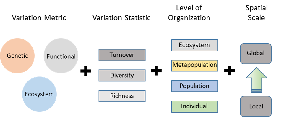
All quantitative descriptions of biodiversity involve four interconnected components (Fig. 2.2). First, there are various metrics of variation that are the basic data units of variation. Those data are summarized using a range of statistics that describe the data in different ways. Each of the metrics is also always observed with respect to specific levels of biological organization and spatial scales.

Variation Metrics

There are three broad classes of biological variation: genetic, functional, and ecosystem. Each class includes a variety of different metrics that use different base units and describe different aspects of the variation. Table 2.1 lists a few of the more common metrics.

Genetic Variation

Genetic variation is the most fundamental form of biodiversity. DNA (deoxyribonucleic acid) and RNA (ribonucleic acid) sequences regulate the form and function of all life. As a result, variation in these sequences underpins much (but not all) of the other forms of variation that constitute biodiversity. Alleles (the different sequence versions of a gene) are examples of genetic variation. Up until the past decade or so, we only had the technology to describe variation in a few genes in a few organisms. But we can now sequence entire genomes relatively quickly and inexpensively, which has led to an explosion in the amount of genetic sequence variation that we have described and quantified.1

Although you may not think about them in this way, species are another metric of genetic variation. Species are genetically distinct units (more or less) whose component individuals are linked by shared heredity. Before we understood DNA or had the tools to describe its variation, we classified organisms into distinct species based on their physical traits and inferences about their degree of relatedness. One of our great scientific advances was understanding that the physical trait-based groupings reflected underlying patterns of variation in DNA and RNA sequences. Even with advances in DNA sequencing, species are still the basic file folder of life and the most tangible form of biodiversity. As of 2022 we have described and cataloged 2.2 million species,2 although the total number of species that currently exist is still just a moderately informed guess. While most estimates place the number of multicellular species in the 8-10 million range, some suggest there could be as many as 100 million eukaryotic species.3 Those estimates probably undercount the tinniest organisms, and they ignore microbial species altogether; one estimate is that there could be as many as 1 trillion of those.4

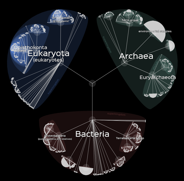
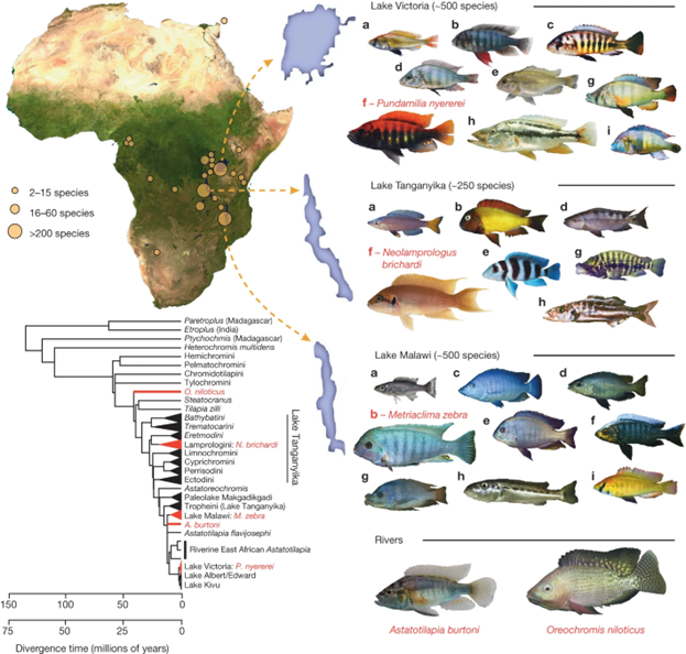
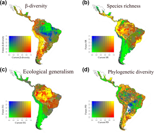
Phylogenies describe how similar (or different) genetic groupings such as species are. They also depict (or at least infer) the pattern of evolutionary relatedness among groups. Figure 2.3 is a phylogenetic tree of life based on genome sequence variation. Short branch lengths and dense nodes indicate closely related groups whose genetic sequences are more similar, while long branch lengths and distantly separated nodes indicate less genetically similar and more distantly related groups. The variability in relatedness among a collection of taxonomic units is called phylogenetic diversity.

Functional Variation

Despite the fundamental role that genetic variation plays in regulating life, it is rather disappointing as a descriptor of life’s variability. Genome sequences, species lists, and phylogenies do a poor job of describing how organisms interact with the world. A species checklist is a lot less interesting than an illustrated field guide complete with descriptions of cool life history and interesting behavior. Variation in these functional attributes—functional variation—is another aspect of biodiversity.

Quantifying interactions is a bit more ambiguous than tallying differences in DNA sequences. One approach is to identify functional traits that directly relate to how organisms interact with each other or the physical environment. These can be physical traits such as color, size, or hairiness. They can be physiological processes such as growth rate or respiration. They can be behaviors such as shyness or intelligence. They can also be cultural knowledge that gets passed down from generation to generation through social learning instead of through genetic heredity.5 Examples of cultural traits include knowledge about where the best feeding grounds are, as well as more lyrical traits such as a cool new song that spreads across humpback whale populations.6

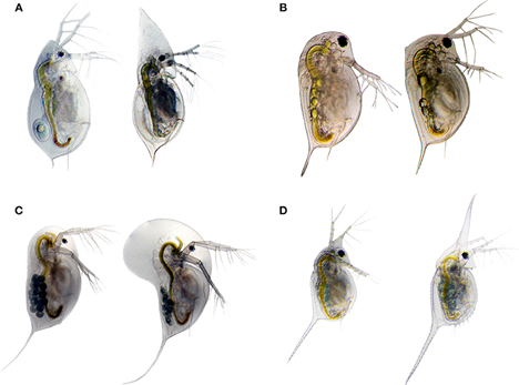
An important aspect of functional variation is that it does not directly correspond with genetic variation. For example, strong selection often causes genetically distant species to converge in traits so that they interact with the environment in similar ways. See the examples of convergent evolution discussed in Chapter 3 (see Fig. 3.7). Conversely, phenotypic plasticity can cause individuals and populations to diverge in traits even though they are genetically similar or even identical. For instance, many organisms have inducible defenses against predators, such as spines or chemical deterrents that they can switch on in the presence of predators (Fig. 2.4).

Functional variation is the most direct description of the ecological functions and processes occurring at a given place. For instance, if you were interested in understanding what factors cause primary productivity to vary across a landscape, looking at the variation in plant traits that influence photosynthesis such as leaf thickness and water use efficiency would be more informative than simply looking at the variation in plant species. Functional traits also reflect evolutionary adaptations to the various constraints and trade-offs that organisms face in trying to survive, grow, and reproduce. The constraints and trade-offs canalize functional variation into distinctive life history strategies. Examples include perennial versus annual plants, carnivores versus herbivores, and semelparity versus iteoparity. Variation in life history strategies is another metric of functional variation.

Ecosystem Variation

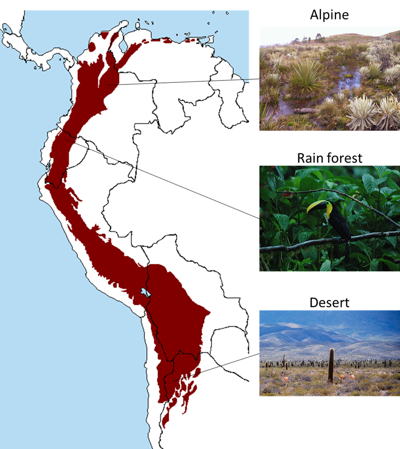
Metrics of functional variation such as life history traits are focused on the ways that individual organisms interact with the environment. But life is also organized into collections of individuals that interact with each other and with different physical environments, known as ecosystems (see Chap. 3). Like the neighbors on your block or in your apartment building, the composition of ecosystems is largely a product of circumstance. Members come and go as circumstances or conditions change. Unlike genetic and functional variation, ecosystems are not direct products of evolution. Still, like species, they are one of the more tangible aspects of the biophysical world. Even if a person can’t identify a single species, they can still probably distinguish a grassland from a forest from a desert. In addition, like functional traits, ecosystems are often a more direct way of describing variation in ecological processes than species are. For instance, deserts have characteristic sets of functional traits (e.g., plants with fleshy leaves, animals with super strong kidneys) as well as levels of ecosystem processes (e.g., amount of primary production, degree of environmental variability) that consistently differ from those of rain forests. The number and variability of ecosystems across landscapes are therefore additional aspects of biodiversity.

Defining ecosystem types is inherently subjective. It can also be maddeningly slippery to define what the boundaries of an ecosystem are and to decide what spatial scale is the appropriate frame of reference. An alternative approach is to instead describe variability in specific ecosystem processes or characteristics that can be more easily defined and quantified using standardized units. Examples include net primary productivity, canopy height, and structural complexity. These are similar to the functional traits of individual organisms, but these ecosystem traits emerge from the collective interactions of ecosystem components as a whole.

Variation Statistics

The variation metrics described above are basic units of variability that we can quantify into data. Like other data, we can use statistical descriptions to help organize the data and enhance our understanding of it. We have developed lots of statistics to describe biodiversity data, many of them sophisticated or complicated. They generally fall into three broad types that describe different aspects of variation. Each can be applied to almost any metric across all three categories of variation:

Richness

Richness is the total number of different types in a given area of whatever variation metric you are looking at (alleles, species, functional traits, ecosystem types, etc.).

Diversity

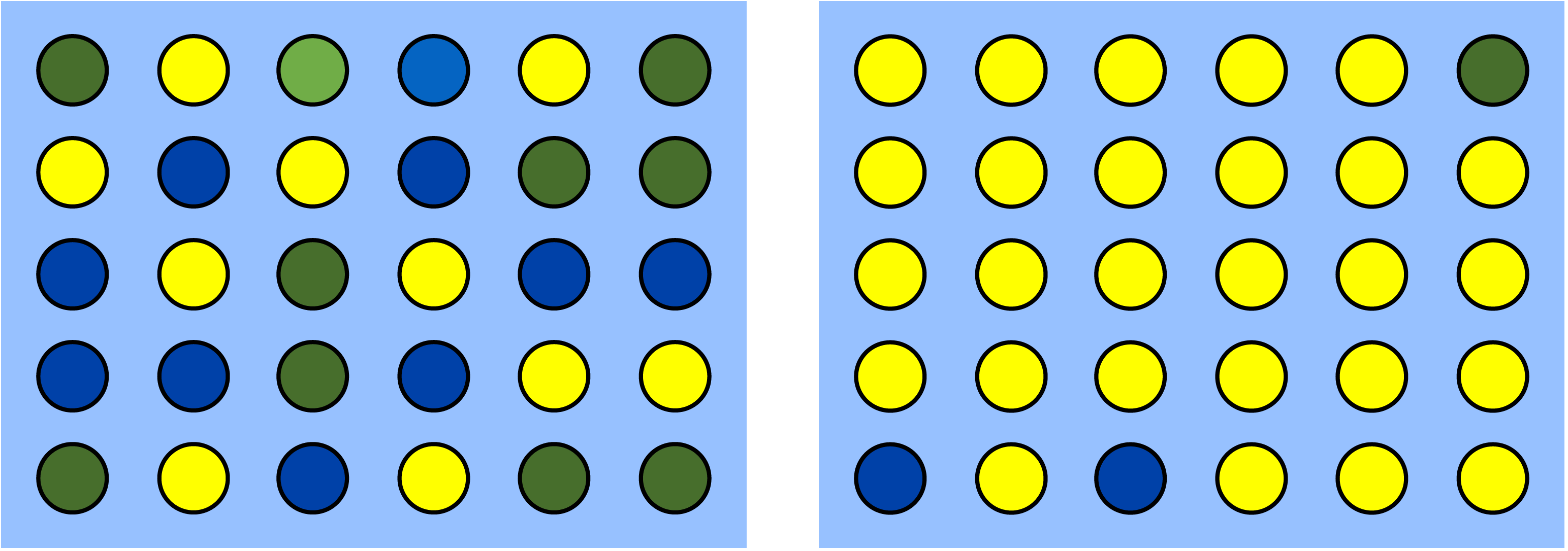
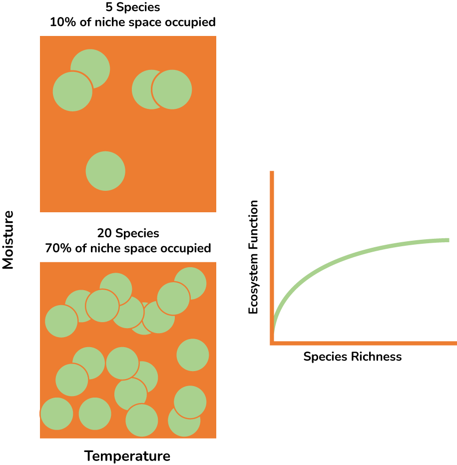
Diversity is synonymous with, well, biodiversity. But technically it is a narrower statistic that describes a specific aspect of variation. Just tallying the number of different types leaves out information about their relative abundance. In any sample, some types are more common than other types. Diversity takes into account both the number of types (e.g., the number of species) as well as the relative abundance of each type. It’s probably easier to see what diversity statistics are trying to describe than read about it. Figure 2.5 schematically depicts two samples that have the same species richness but different species diversity.

Turnover

Turnover is the degree to which variability metrics change as you move from spot to spot across a landscape. I live in an older neighborhood of single-family homes, and it seems like every home has a different landscape design and species composition. Some houses have vast expanses of manicured lawns, others are showcases for evergreen shrubs, and still others are packed full of herbaceous flower beds. Species turnover from yard to yard is high in my neighborhood. In contrast, the adjacent neighborhood is newer and composed mostly of condominiums whose landscapes are managed by a landscaping company. Those landscapes are almost identical one to another. They have the same patch of lawn, the same species of shade tree, and the same species of foundation shrubs. Species turnover from yard to yard is considerably lower in this neighborhood. Although species turnover is different, the average species richness per yard is roughly the same in each neighborhood.

Level of Biological Organization

Metrics of variation are observed and measured at distinct levels of biological organization. Most metrics can be measured at several levels, and each level provides a different perspective on the variation. DNA sequence variation is a great example. We can describe DNA sequence variation at three levels: (1) the similarity of alleles within an individual (zygosity), (2) sequence variability among individuals linked by interbreeding into local populations, and (3) sequence variability across spatially distinct populations linked by dispersal into metapopulations.

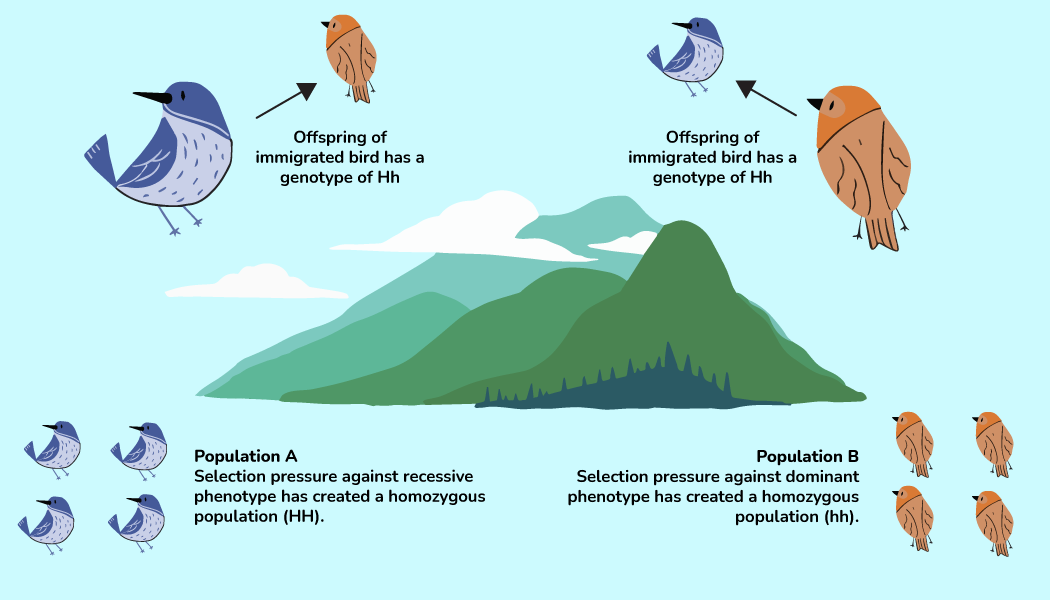
The pattern of sequence variation within and across scales reflects a dynamic balance between gene flow (dispersal + mating), selection, and genetic drift. Figure 2.6 gives a schematic example. The processes can interact in opposing or reinforcing ways, and they often have different effects at different levels of organization. For example, strong selection often reduces the level of genetic variation within local populations because any individuals that don’t have the optimal genotype get quickly selected out. At the same time, strong local selection often increases genetic variation among the populations in a metapopulation because each local population within the metapopulation evolves a unique locally adapted genotype composition. In contrast, gene flow can have the opposite influence. At the scale of the metapopulation, gene flow counteracts the effect of local selection, homogenizing genetic differences among populations. At the scale of a local population, however, gene flow from outside populations can import novel alleles, increasing levels of within population genetic variation. That probably all sounds complicated, and indeed the topic is more deserving of a population biology textbook than this one. But it is a good illustration of how the biological scale at which you observe variation can provide different perspectives. It also illustrates the dynamic complexity inherent in any description of biodiversity.

Spatial Scale

Figure 2.6 illustrates the spatial component of biodiversity. It describes variability at the local scale as well as variability across a larger landscape. To have much meaning, all descriptions of biological variation need to explicitly define what spatial scale the observation was made at. Ten species of plants sounds impressive if it is the number you have in your apartment—not so much if it is the number found across an entire continent.

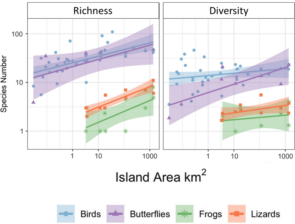
In addition, how variation changes across spatial scales often reflects interesting ecological and evolutionary processes. For example, species richness increases with the size of the area in which you look for species. The positive relationship between species richness and area is one of the most ubiquitous patterns in nature.

Figure 2.7 illustrates an example of the pattern for animal species found on the Andaman and Nicobar Islands. The relationship between species and area partly reflects the effects of increasing sample size—in much the same way that a class of 100 students will have more surnames than a class of 10 students. But the shape of the relationship is also influenced by a range of ecological and evolutionary processes that are specific to different types of organisms and different landscapes. For example, species on isolated islands tend to have smaller ranges than species on more contiguous stretches of mainland. This occurs because each isolated island has evolved a unique set of endemic species with small ranges that differ from other islands, whereas species in contiguous landscapes have more room to spread out and overlap with each other.

As a consequence, species tend to accumulate with area more quickly in patchy island archipelagos than they do in contiguous stretches of mainland. Similarly, landscapes that have more different types of abiotic conditions (e.g., different soils, microclimates) or habitats (e.g., forests, grasslands, wetlands) tend to accumulate species more quickly with area and have overall higher species richness for a given area than do more uniform, less variable landscapes. Different types of organism also have characteristic shapes to their species area relationships. For instance, sedentary species like plants often have steeper species-area relationships than more mobile organism such as birds.

Section 2.2: Why Is there So Much Biodiversity?

The question of where biodiversity comes from and what keeps it around has preoccupied ecologists and evolutionary biologists for a long time. We haven’t figured it all out yet, but we do have a broad understanding of what the main forces are. There are four of them.

Isolation

Metapopulations are inherently unstable. The genetic composition of their constituent populations tends to drift randomly with respect to each other, and they experience selection in different ways. The one thing connecting the populations and unifying them as members of the same species is gene flow. When gene flow between local populations is high, differences get smoothed out and changes affecting one population eventually spread to and influence other populations. But if gene flow drops or stops altogether, local populations grow further and further apart, like two people who have unfriended each other on social media. They acquire distinct genetic sequences and phenotypic traits. Over time, they get so different that a taxonomist is willing to call them different species. Physical isolation that disrupts gene flow has created many (perhaps most) of the species on the planet. The barriers that cause isolation as well as the spatial scale over which isolation occurs depends on the specific life history characteristics of organisms. For example, Alfred Russel Wallace hypothesized that the remarkable species diversity of the Amazon basin was in part a result of isolation caused by the basin’s many river systems that formed barriers to dispersal. This appears to be true for monkeys, who hate swimming; closely related but distinct monkey species can be found on adjacent banks of seemingly modest sized rivers. Rivers aren’t a barrier for many of the basin’s other organisms, however.7

Wallace, (1876) was one of the first people to realize that barriers can shape diversity patterns at the global scale. Continents and major geographic features like the Himalayas are large barriers to dispersal that delineate regions where organisms have evolved in relative isolation from those in other regions. The broadest of these divisions are called biogeographic realms; there are 11 of them for terrestrial animals (Fig. 2.8) and a similar number for plants and marine organisms. Earth’s major geographic boundaries are dynamic . . . well, in the languid geologic sense of the word.

Patterns of geographic isolation shift over long geologic periods. These changes are partly responsible for the fluctuations in diversity patterns that we see in the fossil record. For example, when the Isthmus of Panama rose out of the sea about 3 million years ago, it opened a pathway for the terrestrial species of North and South America to intermix for the first time in more than 60 million years. Species traveled north and south and interacted with each other in various ways in what has been called the Great American Biotic Interchange.8

At the global scale, the exchange reduced species richness because some of the endemic species in each continent went extinct. Extinctions were particularly severe among South America’s unique mammal species. Today, almost half of South America’s mammal genera are descendants from North American immigrants.9[ Species turnover between continents also decreased after the isthmus formed because the faunas of both continents now shared many species in common. At the same time, the migrants tended to increase local richness. During the interchange, for example, species of frogs in the clade Terrarana moved north and south. Today, regions that received the migrants have considerably higher species richness than regions that did not.10 While the Isthmus of Panama created a dispersal pathway for terrestrial species, it formed a barrier to marine species. The isolation caused populations on either side of the divide to diverge genetically, increasing genetic variability at the regional and global scales.11

Selection

Natural selection acting differently on different populations (i.e., differential selection) causes populations to diverge in both genetic composition and functional traits. That makes it a powerful generator of biodiversity. Landscapes that exhibit high spatial variability in environmental condition foster strong differential selection among populations, and they have produced spectacular examples of adaptive radiation. Adaptive radiation is the phenomenon where a single lineage quickly diversifies into many genetically and functionally distinct forms. The adaptive radiation of African cichlid fishes as a classic example (Fig. 2.9). Because gene flow between populations tends to homogenize any differences generated by selection, the ability of differential selection to generate biodiversity is always enhanced by some amount of isolation. The African cichlid radiation was partly the result of periodic isolation caused by fluctuating lake levels.12 Unlike the variability that arises from isolation alone, however, adaptive radiations reflect an increase in both functional variation as well as genetic variation.

If differential selection is strong enough, it can drive diversification without the need for much isolation. The contrasting traits that develop from differential selection can sometimes create their own barriers to gene flow. For example, populations of the California wildflower (Clarkia xantiana) are found across a steep gradient in environmental conditions, and they experience strong differential selection. As a result, populations have evolved distinctive life history types that are associated with specific environmental conditions: ecotypes. Ecotypes from the drier parts of the C. xantiana range have developed a drought avoidance strategy that involves flowering earlier than ecotypes from the wetter part of the range. The difference in flower phenology significantly reduces the chance of cross-pollination between the two types, even in areas where the ecotypes are spatially close to each other.13

Abundant and Variable Resources

In a utilitarian sense, organisms are machines that capture and use energy. As a result, the amount of available energy in an ecosystem sets an upper cap on the number of organisms it can support. The relative availability of energy also seems to influence levels of diversity. There are many examples where biodiversity metrics increase with energy availability.14 A global-scale example is the gradual increase in average local species richness as you move from polar regions to the tropics. We are not exactly sure why the pattern is so common. It seems to partly reflect the fact that energy scarcity usually occurs as a result of severe conditions that test the fundamental limits of organism physiology.

These constraints limit variation in life history or functional adaptations to a narrow set of options that work. As the total availability of energy increases, its spatial and temporal variability also tends to increase. For example, in many extreme arctic habitats, much of the interesting biology is compressed into a few short months of spring and summer. In comparison, many subtropical habitats experience a much more varied and nuanced progression of seasonal changes throughout the year.

Variability in energy supply is just as important in promoting biodiversity as is the total amount of energy, perhaps even more so. Ecosystems that have a range of different types of resources or have temporally variable resource supply often have higher levels of biodiversity compared to ecosystems that have more uniform patterns of resource supply. This is partly because resource variability tends to foster differential selection and isolation. It also potentially creates more ecological niches that are available to be filled by different species and different functional traits. A great example of this is the Cape Floristic Region of southern Africa, which has one of the densest concentrations of plant species on the planet. An area of about 90,000 km² contains more than 9,000 species of plants, 70% of which are endemic to the region.15 This hot spot of plant diversity reflects the region’s uniquely variable conditions. Its soil types are diverse, and they are arranged in an intricate mosaic across the landscape. The landscape itself is dissected and rugged, creating isolation and fostering a complex spatial pattern of microclimates. The regional climate overall is variable in time, marked by a high degree of seasonality and by inter-annual variation. Much of the region is also prone to frequent wildfires that are variable in time, place, and intensity.16

Organisms themselves can modify abiotic conditions, and thus the availability and variability of resources (see Chap. 3.) This can sometimes create positive feedbacks among biodiversity components. For example, reef-building corals modify the flow of energy and materials around them. In effect, their physical structure creates habitat for other species. Corals have a wide variety of structural forms, from large, slow-growing branching types to small, faster-growing crustose forms. As coral structural variation increases on a reef, so does habitat variability. That in turn drives differential selection that fosters increased genetic and functional diversity in other organisms. These feedbacks are probably partly why coral reefs are so biodiverse.17

Time

Biodiversity is dynamic. All its complicated components are constantly changing and rearranging themselves like a kaleidoscope. Amid that complexity, there is one consistent temporal pattern to biodiversity: bouts of biodiversity destruction are usually followed by periods of biodiversity recovery. So, although time is not a biodiversity-generating process by itself, current levels of biodiversity are influenced by how long it has been since the last major period of biodiversity reduction.

Some examples occur over relatively short periods and at local scales when acute disturbances such as a forest fire or volcanic eruption starts the processes of ecological succession. For example, when Mount St. Helens erupted in 1980, it turned a roughly 370 km² area of forest, lakes, and riparian zones into a monotonous moonscape that was almost devoid of life. In the years since, organisms have recolonized, and all of the components of biodiversity have steadily recovered.18

Longer-term and global-scale examples come from the periodic mass extinction events that have taken place over Earth’s history. One of the most dramatic occurred 66 million years ago when a 15-km-wide asteroid slammed into the Gulf of Mexico. The impact ejected a 100-km-wide and 30-m-deep chunk of rock and sediment into the atmosphere. The largest chunks quickly returned to Earth in a fiery rain that roasted large parts of the globe and ignited global forest fires. The smallest particles formed sulfur aerosols in the upper atmosphere, which (combined with soot from the forest fires) blocked solar radiation and dramatically cooled Earth’s climate.19

In the cold, dark world that followed, photosynthesis on land and in the oceans ground to a halt within weeks. One climate model suggests that large parts of the continental landmasses were below freezing for several years.20 About 76% of all species on the planet, including most notably all the non-bird dinosaurs, went extinct.21 Almost as soon as the dust began to settle, biodiversity-generating processes kicked in. The Paleogene period that followed was a time of remarkable diversification both in terms of species as well as functional traits. For instance, about 93% of Earth’s mammal species were wiped out in the immediate aftermath of the impact, but within 300,000 years, local mammal species richness had recovered to levels seen just before the impact, and at the regional scale, richness had doubled.22 The pattern is the same if you look at functional diversity. By looking at insect damage patterns on fossilized leaves, researchers can estimate the richness of herbivorous insect feeding types such as leaf miners, chewers, and gall formers. In both North and South America, the richness of feeding types crashed but then recovered over a period of several million years.23

Section 2.3: Why Is Biodiversity Important?

We derive a great deal of psychological and spiritual joy from ecosystems. Everyone has a favorite species or a favorite ecosystem: part of the natural world they find beautiful or inspirational, something they associate with a loved one or that reminds them of a significant moment in their past, a place that provides meaning. For me, it is the coastal sage scrub habitat of Southern California. Even though I am many miles away from it now, I can still smell the pungent aroma of sage intermingling with the briny Pacific just as vividly as if I was sitting on a bluff in the Santa Monica Mountains. The natural world is also an intricate part of our cultural heritage. Our foodways are a good example. Cherished family recipes, the foods we eat on celebratory or solemn occasions, and our daily eating practices are all strongly influenced by local ecosystems. Ecosystems also provide us with tangible goods and services such as food, medicine, clean air and water, construction materials, storm protection, soil formation and fertility, and nutrient cycling, to name just a few. All of these things help support our well-being: our financial security, our health, our physical safety, our sense of fulfillment, our happiness.

The benefits that we derive from ecosystems are called ecosystem services. They are generated from the ways that organisms interact with the physical environment to drive the flow of energy and materials through the Earth System. Chapter 3 explores how ecosystems function in more detail. But for now, take a look at Figure 2.10. Focusing on coastal ecosystems, it broadly outlines the connection between ecosystem processes, the ecosystem services they support, and the contribution those make to the well-being of coastal communities. Mangroves provide a particularly straightforward example. Mangroves form extensive forests along coastal margins throughout the tropics. Their thick biomass traps sediment and raises the elevation of mangrove-dominated areas. The raised tidal elevation as well as the physical barrier created by the biomass and trapped sediment attenuate the force generated by tides, storms, and even tsunamis, providing valuable protection to shoreline communities. In the aftermath of the 2004 Indian Ocean earthquake and subsequent tsunami, coastal communities that had mangrove forests suffered significantly fewer deaths and property losses than communities that did not have mangroves.24 Coastal protection is just one of the services that mangroves provide. A not-comprehensive list includes timber and fuel wood, breeding and nursery habitat for both marine and terrestrial species, carbon sequestration, nutrient cycling, sediment filtering, and a range of human cultural services.25

It’s relatively straightforward to outline how a specific species or habitat provides a service. But what about biodiversity in aggregate? What is the value of having lots of species, diverse gene pools, and variable ecosystems with rich and complex functions? Assuming there are 10 million species on the planet, would the world get by just fine if there were only 5 million? How about 3 million? We don’t really know. But we have made significant progress in understanding how the individual bits of biodiversity integrate to influence ecosystem function. We have identified several major ways in which the component bits of biodiversity—that is, the variability in alleles, species, functions, ecosystems—come together to create functions and services that are greater than just the sum of individual parts.

Uniqueness and Redundancy

Some bits of biodiversity have a bigger impact on the look and function of ecosystems than others. For example, reef-building corals and large kelp strongly modify surrounding physical conditions and create habitat for other organisms (see Chap. 3). Their presence or absence in an ecosystem therefore has a profound impact on diversity patterns and ecosystem functioning. Other species exert similarly strong influences through their biochemical processes, or because they are inordinately connected to other organisms through their feeding relationships or mutualisms, or simply because they are abundant.

At first glance, it seems that having a few important bits of biodiversity lessens the need for biodiversity in aggregate. Wouldn’t Earth get along pretty well so long as it still had those important bits? But ecosystems don’t get to pick and choose their biodiversity components. Moreover, the importance of any biodiversity element depends on an infinite number of contingencies and unpredictable circumstances. One trait might be incredibly important under one set of circumstances and an arcane curiosity under other circumstances. Instead of reducing the need for biodiversity, such contingent variation in the magnitude of effects among different elements of biodiversity actually enhances biodiversity’s importance. The more different types of alleles, species, traits, ecosystems that are in a landscape, the more likely a particularly important bit of biodiversity is going to be present. Biodiversity also provides a buffer against changing conditions, helping to make ecosystem functions and services more consistent over time than they otherwise would be. Traits that are particularly suited for one set of conditions may not be so great if conditions change. The more variability there is in the components of biodiversity, the more likely that there will be some types that do well in the new conditions. For instance, an allele that conferred heat tolerance might be nondescript when temperature conditions are benign but become important during a heat wave.

From the standpoint of generating ecosystem services, greater biodiversity also produces a greater range of services. Because particular bits of biodiversity help generate particular functions and services such as nitrogen fixation, more biodiverse ecosystems are likely to provide a greater range of potential functions and services than less biodiverse ones. Imagine being on a nerdy reality show where the cast members compete to build the coolest ecosystem service engine. Each contestant receives a box of biodiversity parts from which to build their engine. You would think it unfair if some contestants got boxes filled with many functional types, unique species, and novel alleles while other contestants got skimpy boxes with nothing more than a few common species.

The flip side of uniqueness is sameness. Counterintuitively, sameness can also instill value to biodiversity. This is because ecological and evolutionary processes such as convergent evolution create mismatches between biodiversity components. Genetic variation does not necessarily correspond with variation in functions or variation in ecosystem processes. For instance, a grassland ecosystem might have four or five species that all perform the important function of nitrogen fixation; a coral reef might be constructed from 30 or more reef-building coral species. While these species may perform some redundant functions, they likely differ in a whole range of other traits, such as their environmental requirements. A change in conditions could cause some species to be lost from the ecosystem, but it is unlikely that all the species possessing the redundant function would be lost. This is similar to the types of redundancy that we build into engineered systems like airplanes. Airplanes usually have several redundant yet distinct systems to perform critical functions, such as operating the flight controls. A power failure could cause the electronic flight controls to fail, but the redundant manually operated controls should still work. Traits and functions that are supported by redundant components of biodiversity are more likely to persist in the face of perturbations. That provides a measure of stability to ecosystems and buffers them against changing conditions or the loss of biodiversity.

Complementarity

Species differ in their design. Some are as finicky and temperamental as a finely tuned sports car; others are as robust as a Russian tank. Some like it hot, some like it cold. Some like sandy soil, others are at home in waterlogged muck. Each species has its own unique ecological niche: all the different conditions that define how and when its individuals can extract energy from the environment and convert it into traits, processes, and functions. Sometimes species niches overlap, in which case they tend to compete for the same resources. In other cases, species niches are significantly different, and the species use resources in a complementary way. Figure 2.11 illustrates an example of resource complementarity among insect pollinators in a European meadow. The system contains four broad functional types of pollinators. Each type forages at different vegetation heights and at different times of the day.

Resource complementarity has an important influence on ecosystem function because ecosystems vary considerably in environmental conditions across space and time. From the perspective of the insect pollinators in Figure 2.11, meadows are extremely complex landscapes whose conditions also dynamically change over the course of a day. No single pollinator group can forage equally well across all the range of conditions. Instead, they focus their efforts on the set of conditions under which they have adapted to perform best: low in the vegetation at high noon for solitary bees, early in the morning for hoverflies, high in the vegetation during most of the afternoon for honeybees and bumblebees. From the insect’s perspective, they are optimally foraging for food; from the broader ecosystem perspective, they are optimally performing the ecosystem function of pollination. In aggregate, all four pollinator groups provide more pollination than any single pollinator group would be able to do on its own.26

Facilitation

Resource complementarity is a by-product of species avoiding competition, either by behaviorally adjusting their niche or through the action of natural selection creating specialist adaptations. Species also interact with each other, however, in more directly positive ways that enhance each other’s energy capture or the conversion of energy into processes and functions. Some forms of facilitation are probably just happy accidents of circumstance. For instance, many of the physical habitats created by organisms such as coral reefs and kelp beds probably fall into this category. The habitat conditions they create facilitate energy capture for other species in the ecosystem. These effects are often largest (or at least most visible) in areas with relatively harsh physical conditions that would otherwise be outside the niche parameters of most species. For instance, coral reefs create conditions that lots of other organisms find attractive: a sheltered refuge from waves and currents, an ideal platform for photosynthesis, a solid anchor from which to feed, and a protective refuge from predators.

Other examples of facilitation reflect the more directed action of natural selection adapting species niches to the conditions or resources created by other organisms. For example, some fish species have evolved specialized life histories that are closely associated with the mobile habitat created by sea urchins. Some species use the urchin spines to hide from predators, others to conceal themselves from potential prey, and still others sustainably feed off of the urchin’s tube feet.27 The most evolutionarily refined form of facilitation is mutualism, where species niches have evolved in a reciprocal feedback of mutual benefit.

Mutualisms combine sets of functional traits that would be nearly impossible for either partner to have evolved on their own. Fundamental physical limits and trade-offs constrain life’s possibilities. For instance, the morphology and physiology that are needed to efficiently extract soil resources are different from those needed to convert sunlight into carbohydrates. As a result, natural selection tends to produce organisms whose designs and life histories are compromises. Species can usually do a few things well, they are mediocre at doing many other things, and they can’t do some things at all. Mutualisms sidestep those fundamental constraints and create transcendent combinations of traits.

Mutualisms underlie many critical ecosystem functions that regulate the flow of energy and materials through the Earth System. One of the most important is the mycorrhiza relationship between nearly all terrestrial plants and fungi. Plants benefit from an extensive underground network of fungal hyphae that is remarkably efficient at capturing soil resources such as water and nutrients. The fungi benefit from the plant’s remarkable ability to fix energy via photosynthesis. The evolution of mycorrhiza mutualisms was likely the critical evolutionary innovation that allowed eukaryotic organisms to colonize terrestrial environments.28

Today, much of the energy and materials that flow through terrestrial ecosystems do so via a vast plant-fungus network—a “wood-wide web.”29 As a result, otherwise sedentary and place-bound individual plants and fungi experience and interact with a much wider and more varied environment than they otherwise would. The network allows individuals to share resources and information. The sharing provides a degree of insurance and stability both to individuals and to the network. Parent trees have been shown to support their young seedlings with allowances of sugars and nutrients. Healthy trees have also been shown to help out less fortunate neighbors. Plants under attack from herbivores have been shown to sound the alarm to other plants via the network, giving them time to trigger induced defenses.30

All this sharing may involve as much self-interested skullduggery as it does altruism. The network allows individuals to gather intelligence like a spy agency or an unprincipled baseball team.31 that they can use as leverage to better their own situations. Whatever the motivation, sharing resources and information provides a degree of resilience and stability to the system as a whole that is larger than the sum of its individual parts.32

The Positive Relationship between Biodiversity, Functions, and Services

Conceptually, resource complementarity, uniqueness/redundancy, and facilitation should all foster a positive relationship between biodiversity and measures of ecosystem function. Figure 2.12 illustrates a simple model for how resource complementarity can drive such a positive relationship. Other models make similar predictions for functional uniqueness/redundancy and facilitation. These hypotheses have been supported by a large body of empirical evidence that spans a wide range of ecosystems, spatial scales, levels of biological organization, and all the components of biodiversity. Figure 2.13 provides just three examples. More comprehensive reviews of the evidence confirm how widespread the positive biodiversity-ecosystem function relationship is. For example, a review of hundreds of studies conducted across a variety of ecosystems found that species-rich ecosystems are approximately twice as productive on average (in terms of measures such as net primary productivity) as ones consisting of species monocultures.33 Another review of 258 studies in both terrestrial and aquatic ecosystems found widespread positive relationships between biodiversity and a range of ecosystem functions, including biomass production, pollination, and population stability.34

Keep in mind that ecosystem functions such as biomass production are not necessarily ecosystem services. Services are those ecosystem functions, combinations of functions, or outputs that we value and that support our well-being in some way. Our valuation of specific ecosystem attributes varies depending on any number of circumstances and contexts. For instance, while the biomass production of mangroves produces the ecosystem service of coastal protection, the biomass production of an aggressive weed growing in an agroecosystem is probably not viewed as a service by most farmers. Still, given how much we depend on ecosystems for almost every aspect of our lives, it is usually straightforward to see the connections between biodiversity, specific functions, and our well-being. Each of the functions in Figure 2.13 regulate a range of ecosystem services that in turn support human well-being. Eelgrass beds provide habitat for a number or marine species that support coastal human communities. Similarly, zooplankton biomass supports fish species that support commercial and recreational fisheries. Parasitoids regulate damaging pests in vineyards, reducing the need for costly and dangerous pesticides.

There are many less obvious chains of connection. One example comes from a study that quantified the degree to which species richness made people happy.35 First, researchers asked people to self-evaluate their life satisfaction. This was done as part of a Europe-wide survey called the European Quality of Life Survey that involved more than 26,000 people from 26 countries. Socioeconomic data such as household income were also collected as part of the survey. Researchers then tested the degree to which people’s life satisfaction was related to ecological conditions where they lived, such as species richness and how much open space there was in the neighborhood.

One of the strongest predictors of a person’s happiness was how many bird species were in the region where they lived. Being around many bird species had an even stronger effect on life satisfaction than making more money. Increasing the number of bird species a person was exposed to by 10% led to 1.53 times more life satisfaction than increasing their income by 10%.36 It is not exactly clear why bird species make us (or at least Europeans) happy. Evidence from other studies indicates that listening to birdsongs reduces psychological stress.37 Perhaps hearing a diverse array of beautiful songs improves our well-being more than hearing the same old song from a single bird every day?

The researchers found that other ecological factors were also associated with happiness, such as access to open space, which suggests that nature in general—not only birds in particular—improves our psychological well-being. Interestingly, however, other measures of biodiversity such as mammal and tree species richness were not associated with life satisfaction in this study. The authors speculate that we have a particular affinity for birds because we notice and appreciate their different shapes, interesting behaviors, and beautiful songs a bit more readily than those of more inscrutable trees or reclusive mammals.

A growing number of other studies have documented similar associations between biodiversity and our psychological well-being. One of these tested the relationship between the biodiversity of urban parks and their psychological restorative benefit. The researchers asked people using parks in Bradford, United Kingdom, to rate them based on their overall “restorative benefit.” Restorative benefit includes factors such as how much the park provided a refuge from unwanted distractions and the degree to which the park allowed people to rest and recover their ability to focus. The researchers assessed the biodiversity of each park using various metrics and found that the restorative potential of parks was positively related to their overall biodiversity (Fig. 2.14). The association is strong: 43% of the variability in park restorative potential can be explained by its level of biodiversity. People of different ages, genders, and ethnic backgrounds all placed a similar value on the biodiversity of the park.38

Just as with the connection between bird richness and life satisfaction, we are not exactly sure why more biodiverse city parks provide us with more restorative benefit.

Complexity, Scale, and Other Complications

Although we have made considerable progress in understanding the role that biodiversity plays in generating ecosystem functions and services, there is still much that we don’t understand. One complication is the complexity of biodiversity itself. The exact nature of the relationship between biodiversity, ecosystem function, and ecosystem services varies depending on the specific biodiversity component or metric, the scale of observation, the metric of ecosystem function, and how we define services. In addition, ecosystems vary across space and are dynamic across time. Figure 2.15 illustrates some of that complexity. As we move from spot to spot across a landscape or as time passes, environmental conditions change. The changing environmental conditions influence the mix of organisms as well as the metrics of biodiversity that exist at any location or point in time. All those factors interact to influence ecosystem function. We can also observe conditions at fine-grained scales, or we can aggregate observations and look at regional or long-term averages. The different perspectives of scale provide different pictures of biodiversity-function relationships. Strong positive relationships at one scale can be weak or even turn negative at other scales.39 That type of contextual complexity makes it difficult to apply the knowledge we get from one ecosystem, biodiversity metric, function, or scale to other ones.

Another complication is that the various biodiversity components interact in ways that we don’t understand very well. Moreover, the effects of the interactions play out over a range of scales. An example comes from a study where researchers tried to understand how biodiversity influenced the productivity of forest stands outside of Quebec, Canada. The researchers found that stands with higher tree species richness and functional diversity had higher primary productivity. Resource complementarity among the tree species was probably partly behind the pattern. Tree richness and diversity were not the only factors influencing stand productivity, however. The researchers found that stand productivity also increased with levels of genetic diversity of bacteria living on the tree leaves. Biodiversity of both the trees and the leaf bacteria had independent as well as synergistic effects on stand productivity.40 It is not clear how the diversity of trees and bacteria interact to influence productivity at the scale of the stand. The bacteria community living on tree leaves provides many important functions for the tree, such as protecting against pathogens and helping to fix atmospheric nitrogen. Trees with more diverse leaf bacteria may just be healthier and able to maintain high levels of productivity under a range of different environmental conditions. It might also be that variation in leaf bacteria from tree to tree or across different species of tree enhances resource complementarity among the trees.

Such interactions between groups of organisms and components of biodiversity seem to play important roles in generating the whole complex array of ecosystem functions. For simplicity, we tend to focus on one or a few functions at a time. The examples in Figures 2.13 and 2.14 depict how biodiversity influences one function. But ecosystems are composed of complex suites of functions maintained by complex interactions that we are still in the early stages of understanding. We have made some modest strides for some ecosystems. For example, researchers working in the forests of southeastern China have produced a rough outline of how several different aspects of forest biodiversity influence nine distinct ecosystem functions (Figure 2.16A-B). But each biodiversity-function relationship is part of a far more complex web of interaction among the organisms in the ecosystem. The degree to which the forest ecosystem provides multiple functions reflects the net result of all those interactions. Figure 2.16C depicts how the different biological components of the forest influence each other and the degree to which the forest generates multiple functions.

Some components directly foster more functions, such as the species richness of soil decomposer organisms is positively related to multiple functions. That seems to reflect the important and diverse roles and functions that decomposer organisms provide in this forest ecosystem. The individual biodiversity components also influence multiple functions indirectly through each other, however, and it quickly becomes difficult to interpret what is going on. For example, the functional trait composition of trees positively influences decomposer species richness—and thus indirectly also positively fosters multiple functions. Confusingly, at the same time, tree trait composition also directly inhibits multiple functions. Even more confusingly, the species composition of trees within a stand has a mirror effect. It negatively influences decomposer richness (indirectly inhibiting multiple functions) but also directly fosters multiple functions. We have a way to go before we more fully understand how all the different components of this forest ecosystem interact to influence its range of functions.

Understanding how ecosystems generate multiple functions is important partly because many of our actions tend to create ecosystems that have reduced biodiversity and generate more constrained sets of functions and services. Forests offer a good example. The nine functions listed in Figure 2.16 are still only a subset of the functions and services that biodiverse forest ecosystems provide. Among other things, they also help modulate local climate, regulate the availability of fresh water, suck CO₂ out of the atmosphere and store it for long periods, and provide habitat for a range of plant and animal species, many of which we harvest for food. In general, human-managed and -modified forests around the globe have reduced levels of diversity because we are focused on maximizing the production of a few species with high commercial value, such as Monterey pine (Pinus radiata) or oil palms (Elaeis spp.). As a consequence, these forests often provide fewer and less stable services than more diverse forests. This is even the case if our goal is only the production of the commercial species itself. Single-species plantation forests are more susceptible to disease and insect attack than species-rich forests. Their overall productivity is more susceptible to other environmental vagaries such as drought compared with more diverse forests.41

The important role that leaf bacteria play in the productivity of Quebec forests illustrates another gap in our understanding of biodiversity: we still haven’t described most of it. Most of our understanding of biodiversity comes from plants and animals, which make up a small part of the overall tree of life (Fig. 2.3). We have a comparatively much sketchier understanding of the microorganisms that collectively make up most of Earth’s biodiversity—its microbiome. We have a general understanding that the microbiome plays a critical role in regulating many Earth System processes and functions; mycorrhiza relationships are just one example. Until recently, however, we have had a coarse and superficial understanding of microbiome biodiversity, let alone how that biodiversity influences ecosystem function. That is beginning to change, in part because of a range of new biotechnology techniques that have allowed us to more quickly and easily describe genetic variation in fee-living microorganisms. Projects such as the Earth Microbiome Project are beginning to provide a more comprehensive catalog of Earth’s microbial diversity.42

We are also developing a more comprehensive understanding of how microbial biodiversity influences processes in a range of different systems. Our growing appreciation of the role microbial biodiversity plays in our own health is a good example. Our bodies provide habitats for a rich community of microorganisms known as the human microbiome. We know remarkably little about these organisms or the roles they play among each other and with us. But we are beginning to get tantalizing clues that reductions in our individual microbiome diversity can negatively affect our health. Several illnesses such as inflammatory bowel disease, diabetes, cancer, psoriasis, obesity, and even neurological syndromes such as autism have been associated with reduced microbiome diversity.43 Some treatment therapies, such as fecal transplants, aimed at restoring healthy levels of microbiome diversity have already been developed.44

Section 2.4: Predicting Biodiversity Change

We are rapidly changing the planet and the biodiversity it supports. Because of these changes, the questions we have about biodiversity are not simply quests for understanding—although they are that as well. They are more immediate and mundane. How are we changing biodiversity? What will that mean for our livelihoods and well-being? What will it mean for the planet? Can we do anything to reduce the declines or mitigate the impacts? These questions are difficult to answer, partly because we still know relatively little about how the world works. But we have made enormous gains in our understanding—much of it in the brief few decades since the untimely deaths of Gentry and Parker. In a sense, the rest of this book explores the progress we have made toward answering those questions. One important part of this approach has been the use of models to predict both changes in biodiversity and the consequences of those changes. As the book progresses, many of the examples and evidence will be based on the predictions made by models. As a prelude to that, this section provides a brief overview of the main types of models we use to answer questions related to biodiversity. We have developed many forms of these models, but most of them can be classified into four main types.

Environmental process models

These models attempt to predict how our actions influence environmental conditions such as climate, ocean pH, or ozone levels in the atmosphere. As such, they are not biodiversity models by themselves. But environmental factors have a strong influence on biodiversity patterns, so environmental process models are often used in conjunction with other information or other models to help predict future biodiversity. These types of models are composed of algorithms that describe the key components, processes, and interactions that influence a trait of interest, such as temperature or rainfall. Because the algorithms describe dynamic processes, we can run the models forward (or even backward) in time. We can also adjust the various parameters of the algorithms to see what changes they cause. The best examples of this type of model are the global circulation models used to predict future climate under different greenhouse gas emission scenarios (see Chap. 4).

Ecological niche models

These types of models attempt to predict whether a species can inhabit a particular location given information about its ecological requirements—its ecological niche. For example, each of the hypothetical species in Figure 2.12 has a specific temperature and moisture requirement. If we had a map of moisture and temperature conditions across a landscape, we could identify which parts of the landscape fell within the niche requirements for each species and which did not. In fact, you could view those boxes in Figures 2.12  as physical maps describing spatial gradients in temperature and moisture; species only inhabit that part of the landscape that meets their niche requirements. Ecological niche models usually get their information about the niche requirements of species by describing the environmental conditions that currently exist across current species ranges. Areas currently occupied by species presumably have conditions that meet their niche requirements, whereas areas where species are absent presumably have conditions that fall outside of their niche requirements.

Ecological niche models are often used in conjunction with environmental process models to predict how species distributions might change if environmental conditions change across a landscape. Niche models for multiple species can also be combined to estimate how biodiversity metrics would change under changing conditions. Figure 2.17 illustrates an example from a study that tried to predict how climate change will alter biodiversity patterns of neotropical frogs.45 The researchers created individual ecological niche models and drew current range maps for 2,669 frog species. They then used climate predictions made from global circulation models to predict the range of each species in 2080. Using the future range maps, the researchers then calculated several biodiversity metrics for each roughly 50 × 50 km spot of ground across the Neotropics: species turnover (described as β‐Diversity in the study), species richness, and phylogenetic diversity. They also calculated a measure of ecological generalism that roughly describes the degree to which the species in a specific location have wide ranges and generalized ecological niches. The models predict that many species will shift their ranges into regions such as highlands that are currently outside of their niche parameters. As a result, these locations will experience a net increase in species richness even though some local endemic species will go extinct. The mixing will increase biotic homogenization in some regions, however, and many locations will become dominated by widespread generalist species and have reduced phylogenetic diversity. Another notable finding is that the details of the expected biodiversity changes vary considerably across the diverse landscapes and ecosystems of the Neotropics.

Species-area models

Some of the simplest biodiversity models are based on the species-area relationship. The species-area relationships in Figure 2.7 use total island area as the predictor variable for species richness and diversity. But we can also build species-area curves that are based on the area of specific habitat or ecosystem types that we think are of particular importance or that we know support many species. One of the many ways that we alter biodiversity patterns is by altering habitat for species, such as by converting species-rich tropical forests into relatively species-poor agroecosystems.

We can use species-habitat area relationships as models to predict how reducing the total area of habitat will change species richness or diversity. The top panel of Figure 2.18 gives an example. It describes species-area curves for two functional groups of Neotropical birds: insectivores like yellow warbler (Setophaga petechia) and frugivores like keel-billed toucan (Ramphastos sulfuratus). The area along the x axis is the area of forest habitat in the region. The shapes of the curves in Figure 2.18 are generalized, but they are based on empirical data that researchers such as Ted Parker have collected. We can use these relationships to predict what will happen to the species richness of both groups if the amount of forest habitat in the region changes, for instance, if it is logged or converted to agriculture. In this case, the relationship between forest area and species richness is similar for both insectivores and frugivores, but that is often not the case. Another use of species-area models is to predict how the biodiversity of different groups of species or the species dependent on different habitat types might differentially be affected by reductions in habitat. One of the big advantages of species-area models is their simplicity. Constructing species-area curves is relatively straightforward. Well, at least much more straightforward than trying to completely understand all the complex ecology of biodiverse systems such as tropical forests.

Biodiversity-function models

Biodiversity-function models attempt to predict how changes to biodiversity will affect ecosystem functions. These models are based on experiments or other empirical observations that describe how levels of a biodiversity metric relate to levels of ecosystem function. Figure 2.13 gives some examples. Sometimes this information is incorporated into versions of environmental process models that have biodiversity metrics for specific groups of organisms as parameters. Many global circulation models include the structural and trait composition of vegetation as model parameters that regulate how much CO₂ vegetation sequesters out of the atmosphere, for example.

The biodiversity-function relationships can also be more simply linked to species-area models. The bottom panel of Figure 2.18 is an example. Insectivorous birds contribute to regulating insect populations, while frugivorous birds contribute to plant seed dispersal. Through painstaking fieldwork, we can build species richness-function curves for those two functions. The species-function relationship has a different effect on insect regulation and seed dispersal than the species-area relationship. Insect regulation hardly declines at all until insectivore richness gets very low, then it drops precipitously off a cliff, perhaps because many insectivorous birds are similar and functionally redundant when it comes to eating insects. In contrast, seed dispersal declines linearly as frugivore species richness declines, perhaps because different frugivore species specialize on different types of fruit (hard ones, soft ones, big ones, oddly shaped ones, etc.), so each loss of a frugivore species results in a steady incremental loss of seed dispersal function. In any case, although both insectivores and frugivores are expected to lose similar amounts of species as forest area declines, the expected impacts on insect regulation and seed dispersal are different. As habitat is lost, regional insect consumption isn’t expected to change much at all until most habitat (and the insectivore species that depend on it) is gone. Conversely, seed dispersal is predicted to drop with the first small losses of habitat and steadily decrease as habitat loss increases.

The model Figure 2.18 brushes a lot of details under the rug, but that is part of its beauty. We can use models like it to better inform immediate and pressing decisions even if we don’t have all the details worked out. Still, some of those details can be important. One important detail is whether anybody cares (or should care) about changes to ecosystem functions like insect regulation and seed dispersal. If nobody cares (or realizes that they should care), then we won’t take action to avert the changes. To help answer those questions, we have developed another class of model. These attempt to link ecosystem functions with ecosystem services and how much we value those services. But how do we value ecosystem services?

Section 2.5: Valuing Ecosystem Services

We often don’t explicitly value ecosystem services. In some cases, it is because we don’t recognize the connection between ecosystem functions like wetland biomass production and benefits like coastal protection. Even if we do recognize the connection, it can be difficult to quantify the value of that benefit because many of the services don’t easily work with the various economic tools we have developed to estimate value. To an economist, everything has a price, or a value that reflects how desperately we would work to get that thing or how bitter we would be if we lost it. Markets are a brilliant way of measuring this relative value. But markets only work easily with things that individuals can own or control and then trade for some other things they can own or control. The exchange rate between things (e.g., the amount of bitcoin you can get in trade for a crate of pumpkins) is a measure of the value of both the pumpkins and the bitcoin. Markets also work well when the things we have are easily quantifiable—like a crate of pumpkins. Many ecosystem services don’t meet one or both of those criteria. Services such as the climate regulation provided by the world’s forests are collective benefits that we all share in. Similarly, many of the underlying ecosystem processes and functions that support services—such as the primary production of marine phytoplankton that support fisheries—are difficult for individuals to control and trade. Other services, such as the moment of calm reflection we get from walking through a city park, are difficult to quantify.

Because we often don’t explicitly value ecosystem services, and when we do, the values don’t easily fit into our economic and political systems (such as markets), we frequently make decisions that influence biodiversity—and by extension our well-being—with incomplete information.46 But ecologists and economists have developed a range of new approaches and tools for better valuing ecosystem services and using those valuations to inform ecosystem management.

Approaches to Ecosystem Valuation

Understanding many of the specific ecosystem valuation methods requires a solid working knowledge of economic theory. The broad approaches are much more straightforward to understand, however (Table 2.2).

Willingness to pay is the most direct approach, wherein we try to evaluate how much someone is willing to give up in exchange to acquire a service. As mentioned above, markets are one great way to do this, but many ecosystem services don’t readily fit into market structures. One alternative approach is to simply ask people how much they value something or would be willing to pay for it. An example comes from a study that estimated the economic value of the US National Park System. The authors asked a sample of people how much more in federal income tax they would be willing to pay in order to retain the current national parks. Based on the survey responses, the authors estimated that the total value of national parks to the US public was $92 billion.47

Another approach is to estimate value of an ecosystem service based on its association with an easier-to-value market good. An example of this approach comes from a study that estimated how the proximity to green space affected the sale price of homes in Amsterdam. The study estimated that houses that were adjacent to green spaces such as parks gained a price premium of 2% to 9% over houses that were not adjacent to parks.48

Restoration cost is the cost to refurbish a degraded ecosystem whose ecosystem services have declined. Examples include revegetating old industrial sites and enacting soil erosion mitigation practices in an agroecosystem. This is often the most straightforward way to estimate ecosystem service values, but it is usually also the most inaccurate. It is relatively easy to estimate how much it will cost to remediate contaminated soil or to revegetate a logged clear-cut. But restoration costs more directly reflect things like the cost of labor, fuel, or raw materials than the actual value of the service we are trying to restore. In addition, restoration efforts often fail to completely restore the lost ecosystem functions and services.49 As a result, many restoration costs are considerable underestimates of the true value. This can be particularly true for cultural ecosystem services. For example, in 2020, the mining company Rio Tinto destroyed Juukan Gorge caves in Western Australia during an iron ore mining project. The caves were a sacred site for the region’s Indigenous owners, the Puutu Kunti Kuurama and Pinikura peoples, who have used the caves for at least the past 46,000 years.50 The Australian government ordered Rio Tinto to rebuild the site. But any reconstruction would be a thin ghost of the original site, and the cost of its construction would in no way match the value of the cultural loss.

Substitution cost is the cost of providing (substituting for) an ecosystem service in some other, non-ecosystem way. The classic example of this is water treatment. Many cities are fortunate to have sources of drinking water that require little to no treatment before being used. The clean drinking water is an ecosystem service, and cities such as New York jealously protect the watersheds and aquifers that provide it. With good reason, the cost of building and running water treatment plants to replace that ecosystem service isn’t cheap. In 1997, New York City estimated it would cost $6-8 billion to build (and $500 million per year to operate) a water treatment plant to replace the water purification services it gets from the Catskill–Delaware watershed, the source of the city’s drinking water.51

Avoidance cost is the cost of bad things that didn’t happen because of an ecosystem service. An example are the fewer sick days and hospital visits in cities where air pollution is reduced because of the presence of an urban forest. One study estimated that trees in 86 Canadian cities removed 16,500 tonnes of air pollution in 2010. Using an avoidance cost valuation approach, researchers valued the human health benefits of that removal at $227.2 million Canadian.52 The value of coastal protection is another good example.

Between 1996 and 2016, 88 tropical storms and hurricanes hit the United States. The amount of property damage those storms caused partly depended on how intact the wetlands were where the storms hit. Areas that had more intact wetlands experienced significantly less property damage. Based on that relationship, the average value of wetland coastal protection was estimated as $1.8 million/km2 of wetland.53 In 2017, Hurricane Irma struck the west coast of Florida, a region that had lost 2.8% of its coastal wetlands between 1996 and 2016. That loss resulted in an estimated $430 million more in property damage than would have happened had the wetlands been more intact.54 A similar study estimated that in 2020 the world’s mangroves provide flood protection benefits exceeding $65 billion per year. If mangroves were lost, 15 million more people would be flooded annually across the world.55

Using Valuations in Decision-Making

Estimating ecosystem service values is difficult, particularly if the goal is to get a comprehensive measure of value. The protection that coastal wetlands provide to property is just one of their benefits. Identifying the other services, estimating their values, and figuring out the most appropriate way of adding them together into a comprehensive measure of their overall value is hard—and we have yet to successfully do that for coastal wetlands, let alone the broader biodiversity of the planet.

Still, even incomplete valuations can be valuable tools for making better informed decisions. An example comes from coastal communities in Thailand. Coastal communities can make money from shrimp aquaculture. The economic value of shrimp farming in terms of jobs and revenue is tangible and goes directly into increasing the well-being of folks in the community—for things like school tuition and health care. This creates strong economic incentives to convert coastal habitats such as mangroves and saltmarshes into shrimp farms. In Thailand, and in coastal communities around the word, this has resulted in a precipitous decline in mangroves at the expense of shrimp farms and other forms of aquaculture. But those coastal habitats also have a less tangible—but no less real—value in terms of services, such as providing coastal protection and supporting fisheries. But do those values outweigh the much more direct economic value of shrimp farming?

Researchers attempted to answer that question by estimating the mangrove ecosystem service values in the same cash money terms as the value of shrimp farming.56 They went about it by first documenting the relationship between the number of mangroves present in the region and the level of three important ecosystem services that mangroves provide: storm protection, habitat to support fisheries, and wood products. Next, the researchers used a range of ecosystem service valuation approaches to estimate the value of the services in economic (i.e., cash money) terms. With the shrimp farm and mangrove values in the same units (US dollars), the researchers could then directly compare economic returns in relation to how much of the coastal landscape the community devoted to each activity.

There is an inherent conflict/trade-off. As the amount of shrimp farms increases, the community gets more revenue from selling shrimp, but the ecosystem service benefits they get from the mangroves decrease. Interestingly, the shapes of the area economic return relationships for shrimp farms and mangroves are different (Fig. 2.19). The returns from shrimp farms are at their maximum when all the mangroves have been converted to shrimp farms. As more mangroves are left intact, the net returns from shrimp farming decrease linearly. Similarly, the maximum return from mangroves occurs when there are no shrimp farms and all the coastline is intact mangrove forest.

Unlike the linear value-area curve for shrimp farms, however, the curve for mangroves is asymptotic. Mangroves still provide considerable value even when some of the mangrove area has been converted to shrimp farms. This is likely because wave attenuation (the ecosystem function linked to the coastal protection service) is a nonlinear function of mangrove area. As a result, the highest combined economic return (from both shrimp farms and mangroves) occurs when about 20% of the original mangrove area has been converted to shrimp farms.57 This information may help coastal communities make management decisions that will maximize their well-being. In this case, it seems like having a mix of shrimp farms and mangroves that left intact 80% of the mangroves would be the most beneficial to the communities.

But that information does not provide a perfect solution for communities. The value of coastal protection is typically much more removed from the day-to-day needs of people than the regular stream of income flowing from the shrimp farms. Mangroves do provide some steady income in the form of wood products and the support it provides local fisheries. But those sources of income are small compared to that of shrimp farming. The biggest monetary value that the researchers in this study estimated for mangroves was related to coastal protection. But that coastal protection is more like an insurance policy than an income stream. Just like an insurance policy, it costs the policyholders money in the short term (the loss of income from potential shrimp farms). That loss of income is not overcome by simply showing people data like that in Figure 2.19. This is particularly so for the poorest members of the community who don’t have the economic luxury to do much planning for the future or to invest in the insurance of coastal protection.

You have probably noticed that the ecosystem service valuations mentioned above are all expressed in monetary terms (i.e., cash). This is commonly how they are presented because it is a handy way of comparing the relative value of different things. Also, cash is the fuel that drives many of the socioeconomic dynamics that underlie the great acceleration. Plus, for better or worse, we frame many of our daily decisions in terms of cash value. Still, it is good to keep in mind that value need not be expressed in cash, and it need not be tied to any particular socioeconomic system. In a broad sense, value is simply how much we care about, love, or depend on something. Many people find cash value to be a wholly inadequate way of describing that.

The debate over how to calculate compensation payments to people who lost loved ones in the September 11th attacks is an example. Similarly, many people are uncomfortable with assigning cash value to ecosystem services, and by extension the biodiversity that supports them. For one, assigning definitive value to something can perversely undervalue it. As soon as we assign a cash value to something, we implicitly make it convertible into something else of equal or greater cash value. But would whatever monetary value we assigned to the Sistine Chapel, the majesty of polar bears, or the beauty of the tropical Andes ever truly reflect the moral, spiritual, and existential costs of losing them?

References

5657*Barbier, E.B., Koch, E.W., Silliman, B.R., Hacker, S.D., Wolanski, E., Primavera, J., Granek, E.F., Polasky, S., Aswani, S., Cramer, L.A., Stoms, D.M., Kennedy, C.J., Bael, D., Kappel, C.V., Perillo, G.M.E., Reed, D.J., 2008. Coastal ecosystem-based management with nonlinear ecological functions and values. Science 319, 321–23. https://doi.org/10.1126/science.1150349
21Barnosky, A.D., Matzke, N., Tomiya, S., Wogan, G.O.U., Swartz, B., Quental, T.B., Marshall, C., McGuire, J.L., Lindsey, E.L., Maguire, K.C., Mersey, B., Ferrer, E.A., 2011. Has the Earth’s sixth mass extinction already arrived? Nature 471, 51–57. https://doi.org/10.1038/nature09678
29Beiler, K.J., Durall, D.M., Simard, S.W., Maxwell, S.A., Kretzer, A.M., 2010. Architecture of the wood-wide web: Rhizopogon spp. genets link multiple Douglas-fir cohorts. New Phytol. 185, 543–53. https://doi.org/10.1111/j.1469-8137.2009.03069.x
28Berbee, M.L., Strullu-Derrien, C., Delaux, P.-M., Strother, P.K., Kenrick, P., Selosse, M.-A., Taylor, J.W., 2020. Genomic and fossil windows into the secret lives of the most ancient fungi. Nat. Rev. Microbiol. 18, 717–30. https://doi.org/10.1038/s41579-020-0426-8
5Brakes, P., Dall, S.R.X., Aplin, L.M., Bearhop, S., Carroll, E.L., Ciucci, P., Fishlock, V., Ford, J.K.B., Garland, E.C., Keith, S.A., McGregor, P.K., Mesnick, S.L., Noad, M.J., di Sciara, G.N., Robbins, M.M., Simmonds, M.P., Spina, F., Thornton, A., Wade, P.R., Whiting, M.J., Williams, J., Rendell, L., Whitehead, H., Whiten, A., Rutz, C., 2019. Animal cultures matter for conservation. Science 363, 1032–34. https://doi.org/10.1126/science.aaw3557
12*Brawand, D., Wagner, C.E., Li, Y.I., Malinsky, M., Keller, I., Fan, S., Simakov, O., Ng, A.Y., Lim, Z.W., Bezault, E., Turner-Maier, J., Johnson, J., Alcazar, R., Noh, H.J., Russell, P., Aken, B., Alföldi, J., Amemiya, C., Azzouzi, N., Baroiller, J.-F., Barloy-Hubler, F., Berlin, A., Bloomquist, R., Carleton, K.L., Conte, M.A., D’Cotta, H., Eshel, O., Gaffney, L., Galibert, F., Gante, H.F., Gnerre, S., Greuter, L., Guyon, R., Haddad, N.S., Haerty, W., Harris, R.M., Hofmann, H.A., Hourlier, T., Hulata, G., Jaffe, D.B., Lara, M., Lee, A.P., MacCallum, I., Mwaiko, S., Nikaido, M., Nishihara, H., Ozouf-Costaz, C., Penman, D.J., Przybylski, D., Rakotomanga, M., Renn, S.C.P., Ribeiro, F.J., Ron, M., Salzburger, W., Sanchez-Pulido, L., Santos, M.E., Searle, S., Sharpe, T., Swofford, R., Tan, F.J., Williams, L., Young, S., Yin, S., Okada, N., Kocher, T.D., Miska, E.A., Lander, E.S., Venkatesh, B., Fernald, R.D., Meyer, A., Ponting, C.P., Streelman, J.T., Lindblad-Toh, K., Seehausen, O., Di Palma, F., 2014. The genomic substrate for adaptive radiation in African cichlid fish. Nature 513, 375–81. https://doi.org/10.1038/nature13726
20Brugger, J., Feulner, G., Petri, S., 2017. Severe environmental effects of Chicxulub impact imply key role in end-Cretaceous mass extinction. Presented at the European Geosciences Union General Assembly Conference, Vienna, April 23-28, 2017.
3Caley, M.J., Fisher, R., Mengersen, K., 2014. Global species richness estimates have not converged. Trends Ecol. Evol. 29, 187–88. https://doi.org/10.1016/j.tree.2014.02.002
7Colwell, R.K., 2000. A barrier runs through it . . . or maybe just a river. Proc. Natl. Acad. Sci. 97, 13,470–72. https://doi.org/10.1073/pnas.250497697
31Conklin, M., 2020. There’s No Lawsuits in Baseball: Houston Astros’ Liability for Sign Stealing. SSRN Scholarly Paper 3604268. Rochester, NY: Social Science Research Network.
15Critical Ecosystem Partnership Fund, 2001. Ecosystem Profile: The Cape Floristic Region South Africa. Arlington, VA: Critical Ecosystem Partnership Fund.
49Crouzeilles, R., Ferreira, M.S., Chazdon, R.L., Lindenmayer, D.B., Sansevero, J.B.B., Monteiro, L., Iribarrem, A., Latawiec, A.E., Strassburg, B.B.N., 2017. Ecological restoration success is higher for natural regeneration than for active restoration in tropical forests. Sci. Adv. 3, e1701345. https://doi.org/10.1126/sciadv.1701345
48Daams, M.N., Sijtsma, F.J., Veneri, P., 2019. Mixed monetary and non-monetary valuation of attractive urban green space: a case study using Amsterdam house prices. Ecol. Econ. 166, 106430. https://doi.org/10.1016/j.ecolecon.2019.106430
46Daily, G., 1997. Nature’s Services: Societal Dependence on Natural Ecosystems. Washington, DC: Island Press.
18Dale, V.H., Swanson, F.J., Crisafulli, C.M. (Eds.), 2005. Ecological Responses to the 1980 Eruption of Mount St. Helens. New York: Springer.
23Donovan, M.P., Iglesias, A., Wilf, P., Labandeira, C.C., Cúneo, N.R., 2016. Rapid recovery of Patagonian plant–insect associations after the end-Cretaceous extinction. Nat. Ecol. Evol. 1, s41559-016-0012-0016. https://doi.org/10.1038/s41559-016-0012
51Ellison, K., 2006. New York’s thirst for nature. Front. Ecol. Environ. 4, 56–56. https://doi.org/10.1890/1540-9295(2006)004[0056:NYTFN]2.0.CO;2
17Erwin, D.H., 2008. Macroevolution of ecosystem engineering, niche construction and diversity. Trends Ecol. Evol. 23, 304–10. https://doi.org/10.1016/j.tree.2008.01.013
14Evans, K.L., Greenwood, J.J.D., Gaston, K.J., 2005. Dissecting the species-energy relationship. Proc. Biol. Sci. 272, 2155–63. https://doi.org/10.1098/rspb.2005.3209
9Faurby, S., Svenning, J.-C., 2016. The asymmetry in the Great American Biotic Interchange in mammals is consistent with differential susceptibility to mammalian predation. Global Ecol. Biogeogr. 25, 1443–53. https://doi.org/10.1111/geb.12504
6 Garland, E.C., McGregor, P.K., 2020. Cultural transmission, evolution, and revolution in vocal displays: insights from bird and whale song. Front. Psychol. 11. https://doi.org/10.3389/fpsyg.2020.544929
25Getzner, M., Islam, M.S., 2020. Ecosystem services of mangrove forests: results of a meta-analysis of economic values. Int. J. Environ. Res. Public. Health 17. https://doi.org/10.3390/ijerph17165830
27Giglio, V.J., Ternes, M.L.F., Barbosa, M.C., Cordeiro, C.A.M.M., Floeter, S.R., Ferreira, C.E.L., 2018. Reef fish associations with sea urchins in an Atlantic oceanic island. Mar. Biodiversity 48, 1833–39. https://doi.org/10.1007/s12526-017-0677-4
42Gilbert, J.A., Jansson, J.K., Knight, R., 2014. The Earth Microbiome project: successes and aspirations. BMC Biol. 12, 69. https://doi.org/10.1186/s12915-014-0069-1
16 Goldblatt, P., Manning, J.C., 2002. Plant diversity of the Cape region of southern Africa. Ann. Mo. Bot. Gard. 89, 281–302. https://doi.org/10.2307/3298566
39*Gonzalez, A., Germain, R.M., Srivastava, D.S., Filotas, E., Dee, L.E., Gravel, D., Thompson, P.L., Isbell, F., Wang, S., Kéfi, S., Montoya, J., Zelnik, Y.R., Loreau, M., 2020. Scaling-up biodiversity-ecosystem functioning research. Ecol. Lett. 23, 757–76. https://doi.org/10.1111/ele.13456
*Gooriah, L.D., Davidar, P., Chase, J.M., 2020. Species–area relationships in the Andaman and Nicobar Islands emerge because rarer species are disproportionately favored on larger islands. Ecol. Evol. 10, 7551–59. https://doi.org/10.1002/ece3.6480
47Haefele, M., Loomis, J.B., Bilmes, L., 2016. Total Economic Valuation of the National Park Service Lands and Programs: Results of a Survey of the American Public. SSRN Scholarly Paper 2821124. Rochester, NY: Social Science Research Network. https://doi.org/10.2139/ssrn.2821124
*Holt, B.G., Lessard, J.-P., Borregaard, M.K., Fritz, S.A., Araújo, M.B., Dimitrov, D., Fabre, P.-H., Graham, C.H., Graves, G.R., Jønsson, K.A., Nogués-Bravo, D., Wang, Z., Whittaker, R.J., Fjeldså, J., Rahbek, C., 2013. An update of Wallace’s zoogeographic regions of the world. Science 339, 74–78. https://doi.org/10.1126/science.1228282
2 IUCN. International Union for Conservation of Nature, 2023. The IUCN Red List of Threatened Species Version 2022-2.. Accessed December 1, 2023, https://www.iucnredlist.org
41Jactel, H., Bauhus, J., Boberg, J., Bonal, D., Castagneyrol, B., Gardiner, B., Gonzalez-Olabarria, J.R., Koricheva, J., Meurisse, N., Brockerhoff, E.G., 2017. Tree diversity drives forest stand resistance to natural disturbances. Curr. For. Rep. 3, 223–43. https://doi.org/10.1007/s40725-017-0064-1
40Laforest-Lapointe, I., Paquette, A., Messier, C., Kembel, S.W., 2017. Leaf bacterial diversity mediates plant diversity and ecosystem function relationships. Nature 546, 145–47. https://doi.org/10.1038/nature22399
11Lessios, H.A., 2008. The Great American Schism: divergence of marine organisms after the rise of the Central American Isthmus. Annu. Rev. Ecol. Evol. Syst. 39, 63–91. https://doi.org/10.1146/annurev.ecolsys.38.091206.095815
43Lloyd-Price, J., Abu-Ali, G., Huttenhower, C., 2016. The healthy human microbiome. Genome Med. 8, 51. https://doi.org/10.1186/s13073-016-0307-y
4Locey, K.J., Lennon, J.T., 2016. Scaling laws predict global microbial diversity. Proc. Natl. Acad. Sci. 113, 5970–75. https://doi.org/10.1073/pnas.1521291113
22Longrich, N.R., Scriberas, J., Wills, M.A., 2016. Severe extinction and rapid recovery of mammals across the Cretaceous–Palaeogene boundary, and the effects of rarity on patterns of extinction and recovery. J. Evol. Biol. 29, 1495–512. https://doi.org/10.1111/jeb.12882
37Medvedev, O., Shepherd, D., Hautus, M.J., 2015. The restorative potential of soundscapes: a physiological investigation. Appl. Acoust. 96, 20–26. https://doi.org/10.1016/j.apacoust.2015.03.004
55Menéndez, P., Losada, I.J., Torres-Ortega, S., Narayan, S., Beck, M.W., 2020. The global flood protection benefits of mangroves. Sci. Rep. 10, 4404. https://doi.org/10.1038/s41598-020-61136-6
45*Menéndez-Guerrero, P.A., Green, D.M., Davies, T.J., 2020. Climate change and the future restructuring of Neotropical anuran biodiversity. Ecography 43, 222–35. https://doi.org/10.1111/ecog.04510
36Methorst, J., Rehdanz, K., Mueller, T., Hansjürgens, B., Bonn, A., Böhning-Gaese, K., 2020. The importance of species diversity for human well-being in Europe. Ecol. Econ. 106917. https://doi.org/10.1016/j.ecolecon.2020.106917
* Mimura, M., Yahara, T., Faith, D.P., Vázquez‐Domínguez, E., Colautti, R.I., Araki, H., Javadi, F., Núñez-Farfán, J., Mori, A.S., Zhou, S., Hollingsworth, P.M., Neaves, L.E., Fukano, Y., Smith, G.F., Sato, Y.-I., Tachida, H., Hendry, A.P., 2017. Understanding and monitoring the consequences of human impacts on intraspecific variation. Evol. Appl. 10, 121–39. https://doi.org/10.1111/eva.12436
44Mosca, A., Leclerc, M., Hugot, J.P., 2016. Gut microbiota diversity and human diseases: should we reintroduce key predators in our ecosystem? Front. Microbiol. 7. https://doi.org/10.3389/fmicb.2016.00455
52Nowak, D.J., Hirabayashi, S., Doyle, M., McGovern, M., Pasher, J., 2018. Air pollution removal by urban forests in Canada and its effect on air quality and human health. Urban For. Urban Green. 29, 40–48. https://doi.org/10.1016/j.ufug.2017.10.019
10Pinto-Sánchez, N.R., Crawford, A.J., Wiens, J.J., 2014. Using historical biogeography to test for community saturation. Ecol. Lett. 17, 1077–85. https://doi.org/10.1111/ele.12310
13Runquist, R.D.B., Chu, E., Iverson, J.L., Kopp, J.C., Moeller, D.A., 2014. Rapid evolution of reproductive isolation between incipient outcrossing and selfing Clarkia species. Evolution 68, 2885–900. https://doi.org/10.1111/evo.12488
* Schuldt, A., Assmann, T., Brezzi, M., Buscot, F., Eichenberg, D., Gutknecht, J., Härdtle, W., He, J.-S., Klein, A.-M., Kühn, P., Liu, X., Ma, K., Niklaus, P.A., Pietsch, K.A., Purahong, W., Scherer-Lorenzen, M., Schmid, B., Scholten, T., Staab, M., Tang, Z., Trogisch, S., von Oheimb, G., Wirth, C., Wubet, T., Zhu, C.-D., Bruelheide, H., 2018. Biodiversity across trophic levels drives multifunctionality in highly diverse forests. Nat. Commun. 9, 1–10. https://doi.org/10.1038/s41467-018-05421-z
50Southalan, J., 2020. Inquiry into the destruction of 46,000-year-old caves at the Juukan Gorge in the Pilbara region of Western Australia: Submission 130 to Joint Standing Committee on Northern Australia.
53Sun, F., Carson, R.T., 2020. Coastal wetlands reduce property damage during tropical cyclones. Proc. Natl. Acad. Sci. 117, 5719–25. https://doi.org/10.1073/pnas.1915169117
1Supple, M.A., Shapiro, B., 2018. Conservation of biodiversity in the genomics era. Genome Biol. 19, 131. https://doi.org/10.1186/s13059-018-1520-3
19Tabor, C.R., Bardeen, C.G., Otto‐Bliesner, B.L., Garcia, R.R., Toon, O.B., 2020. Causes and climatic consequences of the impact winter at the Cretaceous-Paleogene boundary. Geophys. Res. Lett. 47, e60121. https://doi.org/10.1029/2019GL085572
30Tedersoo, L., Bahram, M., Zobel, M., 2020. How mycorrhizal associations drive plant population and community biology. Science 367. https://doi.org/10.1126/science.aba1223
* Thompson, P.L., Davies, T.J., Gonzalez, A., 2015. Ecosystem functions across trophic levels are linked to functional and phylogenetic diversity. PLoS ONE 10, e0117595. https://doi.org/10.1371/journal.pone.0117595
33Tilman, D., Isbell, F., Cowles, J.M., 2014. Biodiversity and ecosystem functioning. Annu. Rev. Ecol. Evol. Syst. 45, 471–93. https://doi.org/10.1146/annurev-ecolsys-120213-091917
34van der Plas, F., 2019. Biodiversity and ecosystem functioning in naturally assembled communities. Biol. Rev. 94, 1220–45. https://doi.org/10.1111/brv.12499
26*Venjakob, C., Klein, A.-M., Ebeling, A., Tscharntke, T., Scherber, C., 2016. Plant diversity increases spatio-temporal niche complementarity in plant‐pollinator interactions. Ecol. Evol. 6, 2249–61. https://doi.org/10.1002/ece3.2026
24Vermaat, J.E., Thampanya, U., 2006. Mangroves mitigate tsunami damage: a further response. Estuarine Coastal Shelf Sci. 69, 1–3. https://doi.org/10.1016/j.ecss.2006.04.019
*Vienne, D.M. de, 2016. Lifemap: exploring the entire tree of life. PLoS Biol. 14, e2001624. https://doi.org/10.1371/journal.pbio.2001624
* Wallace, A.R., 1876. The Geographical Distribution of Animals: With a Study of the Relations of Living and Extinct Faunas as Elucidating the Past Changes of the Earth’s Surface. London: Macmillan.
8Webb, S.D., 2006. The great American biotic interchange: patterns and processes. Ann. Mo. Bot. Gard. 93, 245–57. https://doi.org/10.3417/0026-6493(2006)93[245:TGABIP]2.0.CO;2
*Weiss, L.C., 2019. Sensory ecology of predator-induced phenotypic plasticity. Front. Behav. Neurosci. 12. https://doi.org/10.3389/fnbeh.2018.00330
* Wilson, H., Miles, A.F., Daane, K.M., Altieri, M.A., 2017. Landscape diversity and crop vigor outweigh influence of local diversification on biological control of a vineyard pest. Ecosphere 8, e01736. https://doi.org/10.1002/ecs2.1736
38*Wood, E., Harsant, A., Dallimer, M., Cronin de Chavez, A., McEachan, R.R.C., Hassall, C., 2018. Not all green space is created equal: biodiversity predicts psychological restorative benefits from urban green space. Front. Psychol. 9. https://doi.org/10.3389/fpsyg.2018.02320
32Yang, G., Wagg, C., Veresoglou, S.D., Hempel, S., Rillig, M.C., 2018. How soil biota drive ecosystem stability. Trends Plant Sci. 23, 1057–67. https://doi.org/10.1016/j.tplants.2018.09.007
* Zingone, A., D’Alelio, D., Mazzocchi, M.G., Montresor, M., Sarno, D., LTER-MC Team, 2019. Time series and beyond: multifaceted plankton research at a marine Mediterranean LTER site. Nat. Conserv. 34, 273-310. https://natureconservation.pensoft.net/article/30789/
Media Attributions
definition
License
Icon for the Creative Commons Attribution-NonCommercial 4.0 International License
A Natural History of the Anthropocene Copyright © 2024 by John Lambrinos is licensed under a Creative Commons Attribution-NonCommercial 4.0 International License, except where otherwise noted.