Human-Altered Systems
5 Metamorphosis
How Is Changing Climate Changing Ecosystems?
As Gregor Samsa awoke one morning from uneasy dreams he found himself transformed in his bed into a gigantic insect.
—Franz Kafka, The Metamorphosis
Isle de Jean Charles is barely a place. It sits like a mirage hovering just above the Gulf of Mexico. Increasingly, it doesn’t even do that (Fig. 5.1). Flooding is a regular occurrence. The road connecting it to mainland Louisiana disappears during heavy rainstorms and good high tides. The island seems to meld into the sea altogether during big storms. Most of its people have left, leaving behind a few scattered homes and the forgotten remnants of past lives.
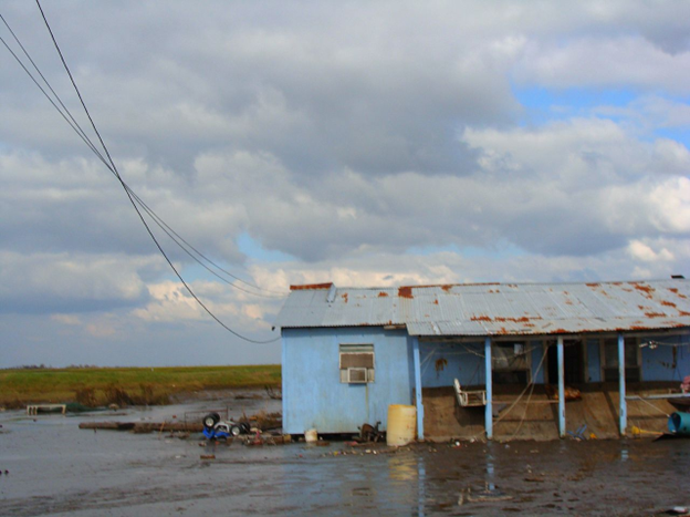
It wasn’t always like this. Granted, it has never been an easy place to get to; the now intermittent road to the mainland wasn’t built until 1953. But it was most definitely a place. A thriving community of about 400 people mostly from the Biloxi-Chitimacha-Choctaw and the United Houma Nation made their living from the vast wetland that surrounded them, one of the largest and most productive on the planet. They fished, harvested oysters, hunted, and farmed. Most of those people have left as the wetland that supported them has died—rather, as we killed it. Past settlers cut a crazy patchwork of channels and canals through the marsh for navigation and to extract oil and gas. Such development helped to foster erosion and created pathways for salt water to intrude into the normally brackish and freshwater parts of the marsh, killing large sections of it. The extraction of oil and gas contributed to subsidence. Humans built dams throughout the vast drainage basin of the Mississippi River that reduced the amount of sediment heading toward the delta, and perhaps most significantly, they built levees within the delta itself that prevented sediment from being distributed across the wetland. Without that rejuvenating supply of sediment and with all our other diminishing actions, the wetland has been eroding away. Louisiana lost about 5,000 km2 of its coastal wetlands between 1932 and 2010.
But the wetland and the people it supports face an even more existential threat. At the same time the wetland has been eroding, the sea level around it has been rising as a result of the warming planet. The combined effects of absolute sea level rise caused by climate change and local subsidence and erosion is causing relative sea level along the Gulf Coast to rise at the rate of about 12 mm per year, one of the highest rates in the world.1
Most of the remaining 85 or so people on Isle de Jean Charles grudgingly know it is time to leave. In 2016, they received a grant from the US government to move the community to higher ground.2 They have been called the country’s first official climate change refugees, but given the multiple factors causing wetland loss, it is perhaps better to think of them as refugees from the Anthropocene. In any case, moving a community—even one as small as 85 people—won’t be easy. Much of the cultural identity of the people of Isle de Jean Charles is tied to the island and the wetland. Tribal elders plan to move representative plants and cultural artifacts like the facade of the town’s old general store, but no one knows what their new community will be like or even if it will survive the move. Many don’t want to find out and vow never to move no matter what.
The residents of Isle de Jean Charles are among the first to feel the consequences of climate change, but they certainly won’t be the last. And it is not just people; plants and animals are also on the move. The whole biota of the planet is undergoing a vast metamorphosis into something new and different. In this chapter, I review some of the ways that climate change is reshaping the ecosystems of the planet that we depend on. I focus on three main parts of the Earth System: the ocean, the cryosphere, and the land.
5.1 Types of Change
Section 5.1: Types of Change
Chapter 4 summarized what we know about how the climate and carbon system work, how we are changing them, and what that is doing to Earth’s physical conditions. Building that collective understanding has been one of our great scientific achievements. But it is only half the story. What are the consequences of those changes for ecosystems and the services they provide us? If we go beyond 1.5°C in postindustrial warming, what will that mean for Iowa farmers? For polar bears? For the primary productivity of the oceans? Answering such questions is a far bigger challenge than understanding climate and carbon flows by themselves.
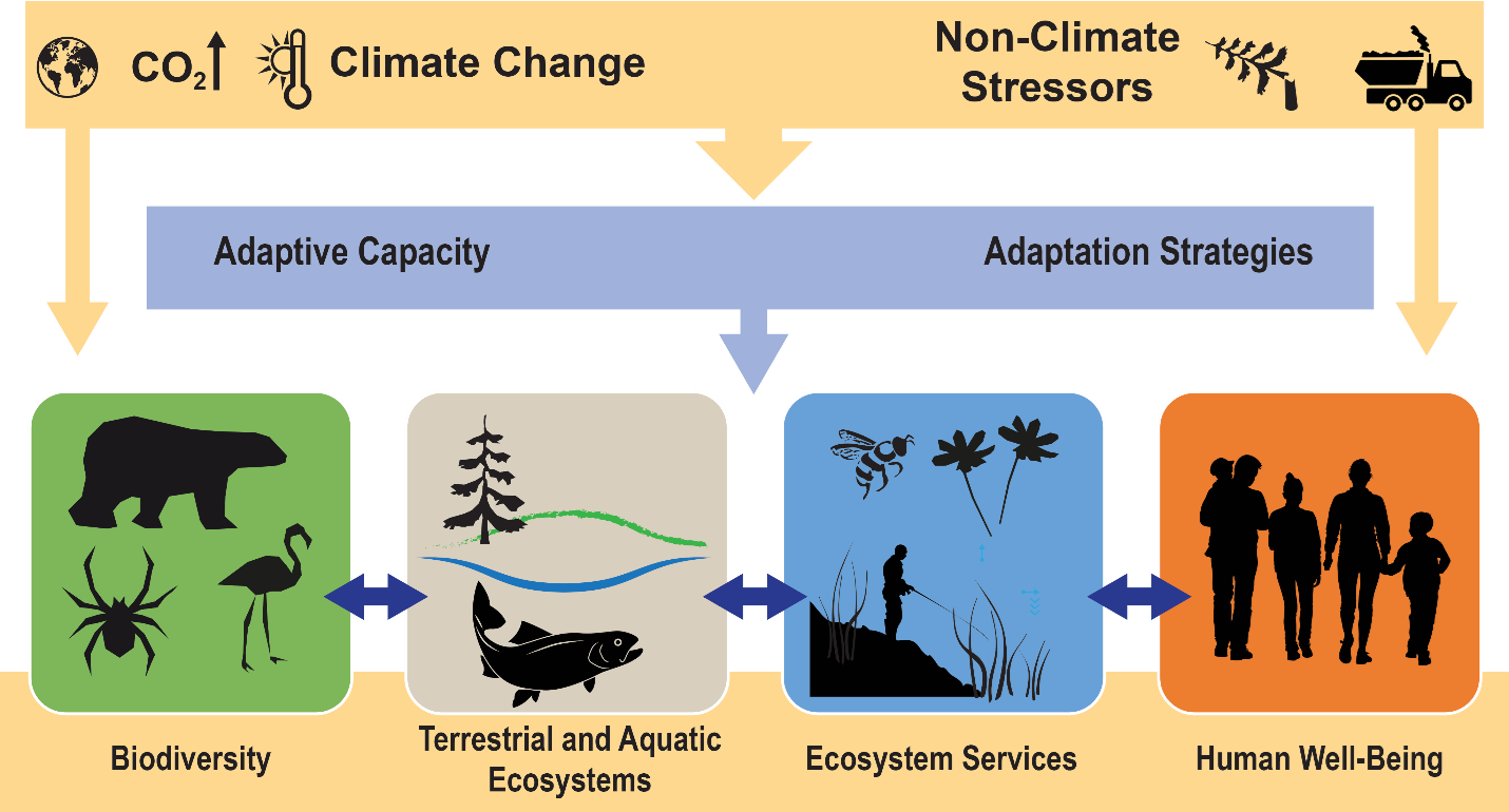
At least on a conceptual level, we know that climate, biodiversity, ecosystem services, and human well-being are interrelated (Fig. 5.2; see also Figs. 2.10 and 3.3). Quantitatively describing all the detailed functional relationships and interactions is technically and logistically challenging, however. In part that is because all the component parts of biodiversity and ecosystems can respond in their own idiosyncratic ways to climate change, and those responses can depend on an array of contingencies such as the peculiarities of local climate conditions, other human stressors such as nutrient pollution, or the historical oddities of how species have come together to form local communities. But imbedded within all that complexity are a few general ways that organisms and ecosystems are responding to climate change. I give just a sketch of these ways here. In the following sections I provide some specific examples.
Behavioral or Physiological Adjustments
As they interact with the world, all organisms can make adjustments on the fly in real time. Two main ways they do this are through behavioral and physiological adjustments. On a hot summer day, for example, we alter our behavior in various ways to cool down—things like wearing shorts instead of black jeans, refraining from physical activity, and drinking more water. Our bodies also adjust physiologically by sweating and increasing blood flow to the skin. These types of adjustments can buffer organisms against direct changes in local climate that may result in conditions such as more frequent hot summer days. They also can help buffer organisms against the indirect knock-on effects that climate change can induce in other parts of ecosystems. For instance, a carnivore might change its diet if its previously preferred prey has gone locally extinct because of climate change.
Range Shifts
A species range is the collection of geographic locations where individuals of that species are likely to be found. Where individuals of a species are found (or not found) is determined by two main things: (1) whether the local environmental conditions are suitable for the species and (2) whether individuals of a species have been able to colonize the location. Neither of those two things is fixed. As climate change alters local environmental conditions, individuals are moving: either to flee newly unsuitable conditions or to take advantage of newly favorable conditions someplace else.
Evolutionary Change and Adaptation
Climate change creates a range of novel conditions that exert selection on individuals within populations of organisms. The adaptations that evolve are another way that organism adjust to climate change. Evolution by natural selection is an inherently slower process than behavioral or physiological responses, but adaptations can sometimes evolve quickly, particularly when the selection is strong. Another way organisms can adjust evolutionarily is by interbreeding and exchanging genes. Climate-change-driven range shifts can bring organisms together that were previously geographically separated from each other. Their new proximity creates opportunities for mating and gene exchange. The gene exchanges can occur between genetically distinct individuals of the same species, or sometimes even when individuals of two different species mate, creating hybrid individuals. Some of the resulting novel gene combinations can be advantageous in the changing conditions, and they can help fuel further natural selection. In other cases, the gene exchanges can be a pathway that causes declines in genetic diversity.
Changing Relationships
No organism is an island. It interacts with other organisms in all sorts of complex and intricate ways. Via the processes above, climate change can disrupt existing organism relationships and create new ones. The possibilities are too detailed to easily summarize. But broadly, the disruptions can alter relationships across the spectrum of interactions, including predator-prey relationships, competition, facilitation, and mutualisms.
Altered Biodiversity Patterns
Climate-driven change can manifest itself in aggregate biodiversity patterns such as the genetic diversity present within a population, the number of species found in a region, or the functional diversity present in an ecosystem.
Altered Ecosystem Functions and Services
All of the changes above can interact to drive changes to collective ecosystem properties, functions, and services. For example, physiological responses by trees to greater summer temperature, the climate-driven range expansion of a wood-boring insect pest, and the climate-driven loss of an important pollinator could combine to reduce primary productivity and fruit yields in a forest.
5.2 How We Measure and Predict Change
Section 5.2: How We Measure and Predict Change
The complex ways that organisms and ecosystems can respond to climate change make it difficult to describe comprehensively how they are changing and even harder to predict what changes might happen in the future. We have made considerable progress using four main approaches, however.
Long-Term Ecosystem Observations
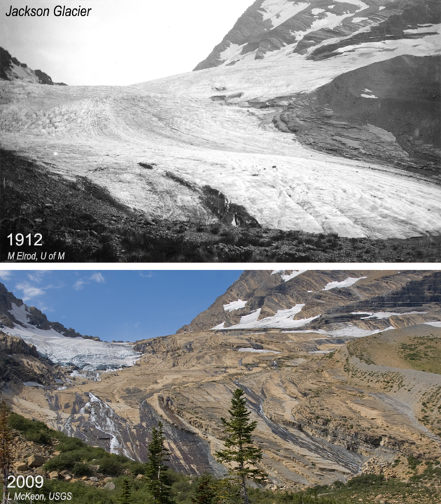
We are beginning to accumulate detailed descriptions of ecosystems that span several decades and in some cases centuries. Many of the longest records come from amateur enthusiasts such as Robert Marsham, who in 1736 began recording the indications of spring on his Norfolk estate in the United Kingdom. These included observations of such things as the first flowering dates of his favorite plants and the first arrival of migratory birds. His descendants kept up the records until 1958.3 Long-term observations such as these are some of the most direct evidence we have documenting how changing climate is altering ecosystems. For example, long-term observations of glaciers have quantitatively documented the rate at which glaciers are retreating as the planet warms (Fig. 5.3).
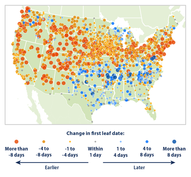
A constraint of these types of observations is that they tend to be focused on just a few ecosystem metrics or limited to a specific location. The Marsham data set, for instance, includes about 27 phenology indicators across about 20 species of plants and animals. But the scope and detail of our ecological record keeping have been increasing. One way we have been doing this is by recruiting a broader range of amateur scientists to help collect the data. An example is a program called Nature’s Notebook that recruits volunteers to record observations of plants and animals in their local communities. The data are then combined with other data to form the US National Phenology Network. There are a growing number of other citizen science projects that collect ecosystem data (see Additional Resources below). On their own, the data collected by citizen scientists help to enhance the spatial and temporal resolution of our ecosystem observations. But they can be particularly useful when integrated with other information. For instance, data from the National Phenology Network helped validate models that were used to retroactively reconstruct the date of first flowering and leaf-out across areas for which we have long-term climate records but not long-term phenology records.4 Those models have shown that spring leaf and bloom dates have gotten earlier across much of the northern and western United States (Fig. 5.4). The growth of citizen science networks has been helped by technological advances such as the widespread availability of Internet-connected mobile devices and automated crowdsourcing platforms such as eBird,5 and iNaturalist.6 The crowdsourcing platforms help to train the volunteers, validate their data, and integrate their observations with other information such as location data.
The development of automated ecosystem sensors has also greatly increased the spatial and temporal scope of ecosystem observations. For instance, satellite-mounted sensors now provide continuous observations of basic ecosystem variables such as chlorophyll levels at remarkable spatial and temporal resolution. In addition, we have increasingly extensive networks of ground-based sensors that provide information that is currently difficult to get without direct on the ground observations. FLUXNET is a global network of sensors that provide ongoing direct measures of the net exchange of CO2 and water vapor between the atmosphere and biosphere.7 Many of these sensors have been collecting data for several decades, which has been enough time to observe the rapid rate of Earth System change. The United States has a dense network of weather radar stations that have been collecting data for several decades. In addition to precipitation, the high-resolution radar also records flying animals such as birds, bats, and even insects. In one study, researchers used a machine learning algorithm to differentiate bird radar signatures from everything else for 24 years of archived radar data. They then used the data to evaluate how the timing of bird migrations has shifted over that time (1995-2018). They found that the peak in spring and fall migration across the United States has been getting modestly earlier, with more pronounced changes during the spring and at higher latitudes.8
Experiments
Long-term observations can document ecosystem change, but if we really want to know what is causing the change, we need to augment the observations with experiments. Experiments can help tease apart the independent and combined effects of different Anthropocene-related stressors on ecosystem traits and processes. Typical experimental designs manipulate one or more environmental variables across a range that climate models and emissions scenarios predict could plausibly occur in the future. These can include climate variables such as temperature and rainfall, carbon system variables such as the concentration of CO2, and other non-climate-related variables such as levels of nitrogen.
Ecosystem response metrics can include nearly any aspect of ecosystems, including the physiological responses of individual organisms, biodiversity patterns, and ecosystem-scale processes such as net ecosystem productivity. Within that general framework, experiments have myriad different designs and span a wide range of scales. At one end of the spectrum are experiments conducted at the scale of individuals and in heavily regulated environments such as greenhouses. These are useful for questions such as how organisms respond physiologically to changing abiotic conditions. At the other end are field experiments conducted at landscape scales. These are useful for testing how changing abiotic conditions influence how organisms interact with each other, alter biodiversity patterns, or alter the biochemical and engineering feedbacks that organisms have with abiotic conditions.
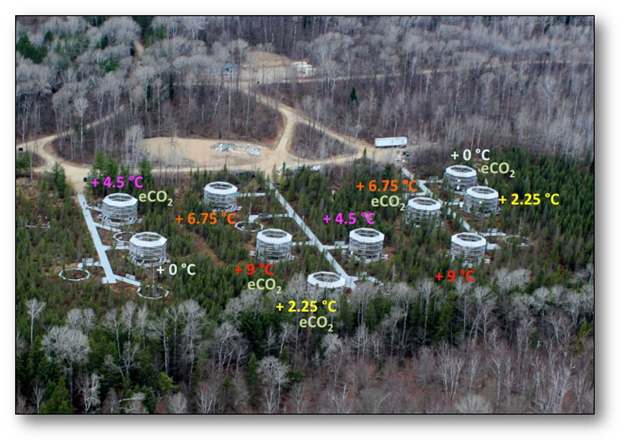
An example of an ecosystem-scale experiment is the Spruce and Peatland Responses Under Changing Environments (SPRUCE) experiment located on a northern Minnesota peatland (Fig. 5.5). Peatlands are currently a large reservoir of terrestrial carbon; although they only occupy 3% of the global land area, they contain about 25% of its soil carbon. But climate change may have pushed peatlands near a tipping point, past which they will become a net emitter of greenhouse gasses instead of a net sink.9
The SPRUCE experiment is located at the southern margin of boreal peatland forests, a location that is likely to be particularly close to a climate tipping point. SPRUCE consists of large open experimental chambers within which scientists can manipulate temperature as well as the ambient level of CO2. The large scale of the manipulations allows scientist to evaluate a wide range of responses, such as changes in the growth of individual species, shifts in species composition, and changes to biochemical processes. Early results from the experiment support the idea that the Minnesota peatland is particularly vulnerable to climate change. Even a modest level of local temperature increase (+2.25°C) turned the peatland into a net carbon emitter, and the rate of emissions increased linearly with further increases in temperature. Carbon losses under the warmed conditions were 4.5 to 18 times larger than the observed historical rates of carbon accumulation for the same peatland.10
The SPRUCE experiment started manipulating conditions in 2015, but other similar experiments have been running for more than a decade. These long-term experiments can provide important insights into how ecosystems progressively change and adapt to climate stressors. In one of the longest-running experiments, researchers have been artificially warming plots of soil in the Harvard Forest since 1991. As of 2016, warmed plots had lost 17% of the carbon in their upper soil layers compared to the unwarmed controls.11 The length of the experiment allowed the researchers to see that the cumulative loss of carbon resulted from complex changes to the soil ecosystem that played out in several distinct phases over the 26 years. Initially, the warmed plots sped up respiration rates of soil organisms, causing a large initial burp of carbon over the first decade. As the initial complement of soil organisms consumed all the easily digestible organic matter, however, rates of soil respiration leveled off and become similar to that of the unheated control plots. During this time, soil organisms became less abundant, and the species composition shifted to groups such as fungi that do well in resource-depleted environments. That quiet phase lasted about 6 years. Then, about 18 years after experimental warming started, respiration in the treatment plots started to increase again. Apparently, this was caused by another shift in the functional composition of soil microbes to forms that specialize in metabolizing particularly hard-to-digest forms of organic matter such as lignin. This second carbon burp was smaller than the initial one, but it involved carbon that would normally have stayed in the soil for a long time. Since 2014, respiration from the warmed plots has again stabilized and entered another quiet phase comparable to the unheated controls.
The results from the Harvard Forest experiment are evidence of a potentially powerful climate feedback. If the soil carbon losses from that experiment are extrapolated across all the world’s forests, it suggests that global warming has caused an aggregate loss of ~190 petagram (Pg) of carbon over just the first couple decades of the twenty-first century. That is equivalent to the carbon emissions from fossil fuel burning over that same period.12 This extrapolation is a crude estimate, though. Forest ecosystems differ greatly from each other in a wide variety of ways. You don’t have to be a forest ecologist to recognize that a pinyon-juniper forest in the arid southwestern United States, a boreal peatland forest in Canada, and a tropical forest in the Amazon basin have different soil carbon dynamics. Because of that variability, we can’t rely on the results from a single location to make accurate predictions at the global scale.
One way to get reliable global estimates is to run the same experiment in multiple places and across different ecosystems. The cost and logistics of doing that are usually beyond the ability of individual research groups or even countries, so instead, researchers often form collaborative networks to share the work and the resulting data. A related approach is to statistically aggregate the results from studies whose designs were not coordinated with each other as part of a cooperative network but are still broadly similar. Researchers took that approach to estimate the potential global loss of soil carbon under climate change. They used as input data the results of 49 separate soil-warming experiments conducted across six biomes, ranging from arctic permafrost to dry Mediterranean forests. As expected, there was a lot of variation in the results: soils at high latitudes and soils that started with the most carbon lost the most carbon under experimental warming. The researchers then extrapolated the results to a global scale, explicitly taking into account the variation across ecosystem types. They concluded that if we follow the high-emissions scenario of representative concentration pathway (RCP) 8.5 (see Section 4.5), it will cause the release of an estimated 55 Pg of soil carbon by 2050.13 That’s considerably less than the estimate of what has already been released based on the Harvard Forest experiment alone, but it still is a significant climate feedback.
Models
Observations and experiments can help us understand how climate and the other aspects of ecosystems interact. We can use that basic understanding to develop models of how the Earth System works, and then use the models to make predictions about how ecosystems and ecosystem services will change in the future if we continue to alter climate. We have developed numerous different types of models that differ in their spatial and temporal scales as well as the questions they are designed to help answer.
The largest-scale models are extensions of the global circulation model (GCM) climate simulations described in Chapter 4. Early GCMs focused on describing the physical drivers that directly influence climate. They tended to treat many of the indirect climate feedbacks involving organisms, such as the dynamics of the carbon system, in general ways. They also did not explicitly describe the impacts of changing climate on the biological parts of ecosystems, such as the abundance or functional diversity of different vegetation types. But advances in computational power as well as in our understanding of the Earth System have enabled us to build more comprehensive Earth System models that describe the biotic-abiotic feedbacks in more detail. The latest Earth System models explicitly describe the role of biological communities in influencing important ecosystem flows, such as those for carbon and nitrogen. Just like GCMs, Earth System models can be used to make future climate predictions under different greenhouse gas emission scenarios. But they can also be used to predict how changing climate will influence biology, such as the distribution of forests or the composition of soil organisms, and in turn how those changes could influence ecosystem services. Earth System models can also be used to evaluate how other Anthropocene stressors beyond greenhouse gas emissions such as nitrogen pollution and land use change could influence climate and the other parts of ecosystems.
One constraint of Earth System models is that they describe big-picture dynamics. Many of the most practical questions about the impact of climate change are at local scales and involve specific parts of ecosystems. For instance, what will wheat yields in the Palouse region of the United States be by midcentury if we maintain our current rate of CO2 emissions? A broad approach to making those types of more specific predictions is to combine the results of GCMs and Earth System models with other models that describe the physiology or ecological interactions of organisms. The first step in doing that is usually to spatially downscale the climate predictions to more local scales. Even the latest high-resolution GCMs and Earth System models don’t take into account local details such as topography that can have a big influence on local climate. We can use other models to translate the regional-scale outputs of climate models into more local-scale predictions. The next step is to develop models that describe how local species or ecosystems will change under the predicted future local climate.
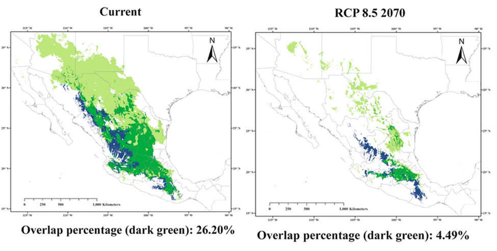
In concept, almost any type of ecosystem response can be modeled, but most of the models that have been developed so far focus on a few species. That is partly because we still have a relatively poor understanding of how climate will alter the complex relationships among organisms and how those combine to shape ecosystem scale properties, although studies such as the SPRUCE experiment are helping to fill in our understanding. The single-species models are called environmental niche models (ENM) because they describe the important environmental factors that make up a big part of a species’ niche. The environmental factors that are most often used are aspects of climate such as temperature and water requirements, although any factor making up the ecological niche of an organism can be incorporated into the model. Niche models have been particularly useful for questions involving the spatial range and distribution of organisms. For instance, they have been used to predict where native species are likely to be found, where non-native species would likely expand to if they were introduced, and where it would be good to grow particular crops. We can use the niche models to predict how the spatial arrangement and distribution of species will likely change under the climate predictions made from GCMs. For example, every spring, the Mexican long-nosed bat (Leptonycteris nivalis) migrates from central Mexico to the southwestern United States, following the progressive blooms of one of its favorite food sources, agaves (Agave spp.). Using climate predictions and ecological niche models, researchers predict that the suitable habitat for bats and agaves (and thus their geographic ranges) will shrink. In addition, the range of the Mexican long-nosed bat will tend to shift southward, while the ranges of many agave species will tend to shift northward (Fig. 5.5). This will leave many agave species without access to an important pollinator. The disruption of the bat-agave pollination system would have profound consequences. Agaves are culturally and economically important species, with tequila being just one product they provide.
Environmental niche models can also be formulated to understand how climate change could influence other aspects of organism performance. An example comes from the arid Columbia Plateau region of eastern Washington and Oregon. Wheat is a major crop here, and much of it is grown without irrigation despite the region receiving less than 300 mm of precipitation a year. This is possible because most of that precipitation falls from fall through spring. Farmers can plant a crop in the early fall, and the first rains will allow for germination and establishment. The young wheat then hangs out for the winter before completing its growth in the spring and early summer using stored soil moisture. As you might expect, this winter wheat system is particularly sensitive to the precise timing and amount of rainfall as well as temperature during a few critical stages in the wheat’s development, all of which could be altered by climate change. Researchers assessed the climate risk by developing models that described how the growth and development of wheat are influenced by environmental variables such as spring soil water availability and early-summer temperature. The models allow the researchers to simulate how different temperature and rainfall scenarios would affect wheat growth and eventual grain yield. The researchers then used climate models to develop local-scale predictions of future climate under different emissions scenarios. The combined models predict that climate change (using the typical set of emissions scenarios) will likely actually increase wheat yields in the region. The yield increase partly results from a predicted increase in winter rainfall and temperature that will improve wheat growing conditions. It also partly results from improved water use efficiency in the wheat related to the CO2 fertilization effect.14
Comparisons to Past Climate
One limitation is that it can be difficult to construct accurate models that describe how whole diverse communities of interacting species will be influenced by climate change. We can sometimes look to the past to get a synthetic picture of how whole ecosystems respond to changing climate, however. Researchers are starting to develop a clearer picture of what past climate and ecosystems were like, and we can use that past as an analogy for future ecosystems. For example, about 53 mya, CO2 in the atmosphere spiked to about 1,400 ppm over the remarkably short time span of about 20,000 years. We are not sure what caused the spike, but we are reasonably certain that it made the world very warm—about 14°C warmer than global temperature at the start of the agro-industrial revolution.15 This warm period is known as the Paleocene–Eocene Thermal Maximum (PETM). The rate and magnitude of the CO2-driven increase in temperature during this time were similar to current changes in the climate, although today’s rate of CO2 increase is about 10 times faster.16 Still, it is a reasonable model to use as a comparison. Paleontological evidence from the Bighorn Basin of North America indicates that during the PETM, local biological communities rapidly rearranged themselves as some species died out locally and new species immigrated to the area. We can also discern shifts in ecological interactions from the fossil record. By quantifying how the frequency of chewed and mined leaves changed over the period, researchers could see that rising temperature led to increased intensity and frequency of insect herbivory on plants.17
Progress in Understanding
Using all four of these approaches, we have begun to make progress in untangling the profound metamorphosis in our planet that climate change is triggering. For some parts of the biosphere, we have developed at least a broad and general understanding of how climate change will likely alter ecosystem processes, disrupt ecosystem services, and affect our well-being (see Fig. 2.10). The following sections represent an exploration of the evidence.
5.3 Troubled Ocean
Section 5.3: Troubled Ocean
The ocean has absorbed 30% of the CO2 we put into the atmosphere since 1880 and 90% of our extra heat.18 Perhaps second only to the cryosphere, it is where climate change is causing its biggest and earliest impacts. The trouble is, compared to terrestrial ecosystems, we know little about the ocean. For many parts of our terrestrial world, we have richly detailed data sets describing ecosystems that stretch back many decades. In contrast, there are considerable parts of the ocean that humans have never seen, let alone studied and documented. As a consequence, we have few equivalent data sets for the oceans. Even basic physical data such as water temperature and salinity had been difficult to collect until the deployment of Earth-observing satellites beginning in the late 1990s. This lack of information hobbles our ability to understand precisely how we are altering marine ecosystems. But what we do know is troubling.
Declining Alkalinity
Seawater has been slightly alkaline for at least the past 425 million years. For at least the past 10,000 years, the average pH of the ocean has been a remarkably steady 8.2.19 It takes a big perturbation to change ocean pH because it is a sink for lots of bicarbonate (HCO3–) and other anions weathered from rocks (equations (4.5)-(4.6)). The preponderance of anions makes seawater alkaline, and because they sop up lots of free hydrogen cations, they also provide strong buffering against changes in pH. Although it takes a strong perturbation to change ocean pH, it has changed significantly at times in the past. Those changes have usually been accompanied by major changes in marine biodiversity. We are currently observing one of these rare and transformative pH changes in real time. In just over a couple hundred years, average ocean pH has dropped to 8.1. That doesn’t sound like a big change, but keep in mind the logarithmic scale of pH; the drop represents a 30% decrease in alkalinity. As CO2 dissolves in seawater, it creates a lot of hydrogen ions (equation (4.4)). Initially, the buffering bicarbonate can easily absorb all the hydrogen ions, but as more CO2 dissolves, free hydrogen ions begin to accumulate and ocean pH declines. This phenomenon is commonly referred to as ocean acidification. Note, however, that the ocean is still alkaline, just less so.
A change in pH this big so quick has stressed almost all marine life. Many marine organisms maintain the pH balance of their internal fluids by regulating the uptake of bicarbonate. As pH drops, they must expend more energy to maintain proper internal pH. Some studies have shown that juvenile fish exposed to lowered pH have significantly reduced growth and survivorship, while the adults suffer a range of behavioral problems, such as an impaired ability to detect predators and to remember their way around a reef. Reduced pH also hampers the ability of fish to deal with other stresses, such as periods of reduced oxygen.20
In addition to stressing the acid-base balance of marine organisms, lowered pH makes it much harder to build calcium carbonate shells. Calcifying organisms have a wide range of important roles and functions that include supporting the base of marine food webs (e.g., calcareous phytoplankton and zooplankton), providing important food for organisms at higher trophic levels (e.g., oysters, mussels, urchins, crabs), and acting as strong ecosystem engineers (e.g., reef-building corals). Any negative impacts on calcifying organisms will ripple through marine ecosystems—and our own communities. We still don’t have a detailed understanding of how marine calcifiers build their shells, but we know the process starts by moving calcium and bicarbonate ions from seawater into their tissues. That is the relatively easy part, because in most parts of the ocean, seawater is usually saturated with calcium and bicarbonate. But most calcifying organisms need to convert bicarbonate to carbonate to form calcium carbonate. This creates hydrogen ions that organisms must get rid of; otherwise, the hydrogen would just bond with carbonate to form bicarbonate again (the reverse pathway in equation (4.4)). They do this by spending energy to pump it out of their tissues. The more hydrogen ions that are floating around in the ocean, the harder organisms need to work to pump hydrogen ions out of their tissues and keep carbonate from turning into bicarbonate.
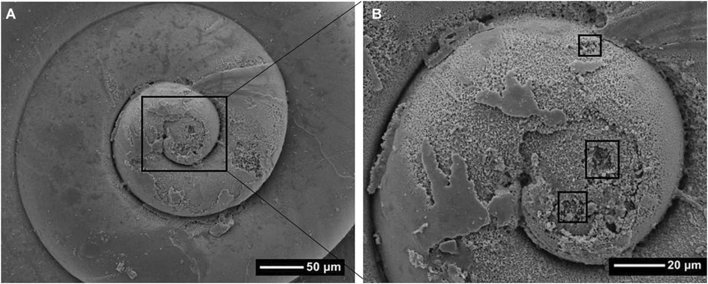
The increasing workload caused by the drop in ocean pH has strained the metabolic energy budget for many calcifying species and has caused calcification rates for many of them to decline.21 Reduced calcification is bad enough—it leads to thinner shells and makes individuals more susceptible to predators like oyster drills (Urosalpinx cinerea). But studies have shown things can get much worse. As pH declines, building shells gets increasingly more difficult, first resulting in malformations and development failures in early life stages, and eventually causing shells that dissolve altogether as the high concentration of hydrogen ions begins to drive the calcification process in reverse.2223 This is already happening to the shells of calcifying zooplankton species. One of the first observations came from pteropods in the Southern Ocean. In a few locations, strong upwelling causes deep, relatively low-pH water to mix with human acidified surface waters, creating local patches of relatively low-pH water. Pteropods collected from these patches had thin and pockmarked shells indicative of dissolution.24 Severe and widespread pteropod shell dissolution has also been observed at the opposite pole in the Amundsen Gulf of Canada, suggesting that the conditions promoting dissolution are becoming more widespread (Fig. 5.7).
We are still in the early stages of understanding what the impact of ocean acidification on marine calcifers and the broader ecosystems of which they are part will be. There is a lot of variability among species. For example, some species of coral can use bicarbonate instead of carbonate to build their skeletons, and this may help them mitigate some of the impact.25 All the variability in species responses makes it difficult to assess how diverse communities of calcifying organisms will respond in lowering pH. One approach that has been used to understand how whole assemblages will change is to look at marine habitats that already have naturally reduced alkalinity. For example, CO2 emitted from hydrothermal vents can reduce the alkalinity of surrounding water. The benthic communities living around natural CO2 vents off of Ischia, Italy, are less structurally and taxonomically diverse than nearby communities that are exposed to more normal ambient pH. Instead of a diverse mix of species that includes many calcifiers, the vent communities have a less diverse assemblage dominated by polychaetes, seagrass, and brown algae.26
Similarly, coral reefs near CO2 seeps off the coast of New Guinea look dramatically different than nearby reefs that lack seeps. Seep reefs are dominated by structurally simple coral species such as boulder forms, and they lack more structurally complex forms like branching species. The boulder forms seem to be particularly resilient to lowered pH; they have been found at locations where the ambient pH was as low as 7.8, although they experience reduced calcification rates under those conditions.27 That suggests coral reefs could potentially persist in some form except under the most extreme pH conditions, albeit at considerably reduced complexity and diversity. That’s somewhat reassuring, but lowered pH is just one stressor affecting coral reefs.
Declining Coral Reefs
Coral reefs are among the most biodiverse places on the planet, but indicative of how little we know about the oceans, we aren’t sure just how diverse. Estimates of species diversity range from 600,000 to more than 9 million, but recent studies using DNA barcoding suggest even the high end of that range might be a severe underestimate.28 Reefs directly support a quarter to a third of all marine species, an amazing number given that reefs occupy less than 0.2% of the ocean’s surface area.29 Reef biodiversity in turn supports a range of ecosystem services, including sustaining many of our fisheries, protecting our coastlines from storm damage, and generating revenue and psychological rejuvenation from tourism.30 Yet despite their importance to us (or perhaps because of it), we have a habit of abusing them. We have overfished them using destructive practices such as dynamite and cyanide, we have introduced species such as lionfish (Pterois spp.) and crown-of-thorns starfish (Acanthaster planci) that kill coral and disrupt food webs, and we have polluted coastal waters, feeding destructive algae blooms and clouding the water with sediment.31
But the most existential threat to coral reefs is the CO2 we are adding to the atmosphere and eventually the ocean. Like other calcifying organisms, reduced ocean alkalinity is making it more difficult for reef-producing corals to make their calcium carbonate exoskeletons. Estimates suggest that many reefs will stop growing altogether and begin to dissolve if atmospheric CO2 reaches 560 ppm. Even assuming some resilience and adaptation on the part of coral species, 750 ppm CO2 appears to be the upper limit for ecosystems that we would recognize as coral reefs.32 But the bigger immediate stress to coral reefs comes from the warming associated with the rising atmospheric CO2. Shallow-water coral species have evolved a close symbiotic relationship with single-celled algae called zooxanthellae. The algae contribute carbohydrates to the coral while getting a place to safely hang out within coral cells. The relationship is sensitive to temperature. Moderate heat waves that push temperatures just 1°C to 2°C above the average summer high for a few weeks cause zooxanthellae to die or get expelled from coral cells. This phenomenon is known as coral bleaching because without their zooxanthellae, coral turn a blanched white (Fig. 5.8). At the very least, bleaching results in slowed growth and reduced reproduction, but it also often results in death.
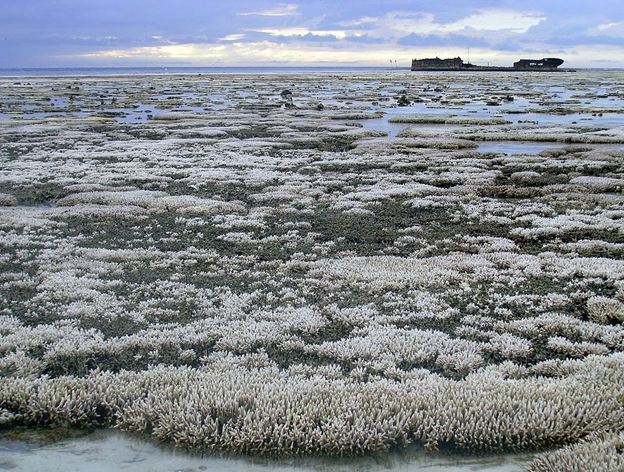
The frequency and intensity of bleaching events have been increasing. Periodically extensive and widespread bleaching was first noted as a regional phenomenon in 1983. In 1998, tropical coral reefs around the world experienced bleaching. That first recorded global bleaching event was followed by another global event more than a decade later, in 2010. Then, from 2014 to 2017, tropical reefs around the world experienced a prolonged period of successive bleaching events.33 The severity, extent, and timing of the bleaching events over that period varied a bit from region to region. One of the hardest-hit regions has been the Great Barrier Reef of Australia. During a 2016 bleaching event, more than 90% of the Great Barrier Reef suffered some bleaching, and almost half of the entire reef system experienced severe bleaching, defined as areas where more than 60% of the coral bleached (Fig. 5.8).
Since 2016, the Great Barrier Reef has so far suffered two more mass bleaching events, in 2017 and 2020. The rapid succession of severe stress has already dramatically changed the species composition of the reef and caused a disquieting decline in the recruitment of juvenile coral. This has caused some scientists to warn that the entire Great Barrier Reef ecosystem may be on the verge of collapse.34 The Great Barrier Reef is not alone. Globally, the combined effects of climate change, ocean acidification, and other reef stressors have significantly altered reefs and degraded their capacity to provide ecosystem services. One study estimated that between the 1950s and early 2000s, the global coverage of living coral declined by 50%, and the effort-adjusted catch of coral reef fish decreased by 60%.35
Range Shifts
Marine organisms are tracking the spatial shifts in abiotic conditions. Species are generally shifting their ranges poleward following the broad geographic shifts in water temperature (see Section 4.4). On average, species have been swimming or floating poleward at the rate of 75 km per decade, much faster than the average 17-km-per-decade shift observed for terrestrial species.36 That might be because ocean currents act as fast-moving dispersal highways for marine organisms, many of which have planktonic life stages. Some species are also shifting their range deeper in the water column, where temperature is cooler. Moving modestly deeper is a fairly common pattern, but it is an inherently constrained strategy. Species quickly face physiological limits of pressure and light that limit how deep they can go.
As climate change continues, the number, pace, and geographic extent of range shifts are expected to intensify, redrawing the biogeographic map of marine biodiversity.37 The tropics will likely lose a big chunk of their species, but most regions at higher latitudes will likely gain species as they take in climate migrants. As a result, many temperate regions will likely see an increase in local biodiversity. All that reshuffling will also tend to homogenize global diversity, making marine communities across different regions look much more similar to each other than they do today.
There is a lot of biological detail embedded in those general patterns. Range shifts can occur either because ranges expand or contract along the equatorial (warmer) edge of the range, or they expand or contract along the poleward (cooler) edge of the range. The sum of those two vectors determines whether the overall size of a species range is shrinking or expanding and in which direction. The net speed and direction of range shifts vary tremendously across species and regions for a variety of reasons. One reason is that the ocean is spatially more complex than most of us land lubbers appreciate. Intricate current systems, particularly those along the margins of continents, define often abrupt boundaries in abiotic conditions that form barriers to species movements. Currents can also go in the opposite direction from that in which habitats are shifting, hindering movement. Coastlines themselves act as barriers that funnel range shifts in particular directions or prevent them altogether. In the Gulf of Mexico, for example, the east-west-running coastline has prevented species from shifting their range northward. Instead, many species have shifted their range deeper in the water column.
Wind and ocean currents also create regional microclimates that can either enhance or counteract the general climate-driven changes in ocean warming. The eastern boundary upwelling systems where ocean water has remained relatively cool even in the face of general ocean warming are good examples (see Fig. 4.11).
Species also vary in their need and ability to move. How fast and even if species can adjust their range is partly determined by their specific life history traits such as growth rate, dispersal ability, and the degree to which they can tolerate a range of abiotic conditions. For example, dinoflagellates and copepods are two major components of plankton at the base of the marine food web. While both groups shift their range in response to climate change in the same direction, diatoms move much more slowly. Individual species also differ in their ability to tolerate changes in local conditions, and that can influence when and how quickly their range shifts. Species that have specific climactic requirements tend to adjust their range more quickly than those that can tolerate a broader range of conditions.38
Disrupted Ecological Relationships
Climate change can alter other aspects of an organism’s life history. These in turn can alter how species interact with each other. Phenology, the timing of periodic life events like spawning, is a good example. At high latitudes, phytoplankton abundance peaks during the spring when the nutrient-rich, well-mixed water of winter combines with the increased light levels and warmth of approaching summer. Many zooplankton that feed on the phytoplankton then peak in early summer, just after the peak in phytoplankton. Within that broad pattern, individual species have evolved exquisitely nuanced timing to take maximum advantage of food resource supplies and to avoid predation. Just as with range shifts, climate change can affect the phenology of each species differently.
Organisms differ in the specific environmental cues they use to place themselves in the phenological calendar. Those differences can create problems in a warming world. For instance, species that primarily use temperature as a cue can get out of sync with species that primarily use day length as a cue. This has been the case for the Baltic macoma (Macoma balthica), a small clam living in the coastal waters of northern Europe. The clams use seasonally warming water temperature in spring as a cue to initiate spawning that will coincide with the spring bloom of phytoplankton. The clams time their spawn a bit earlier than the peak in phytoplankton to give their eggs time to hatch and to put the emerged larvae right in the thick of the food boom. Warming water in the region has moved up the average spawning date for Baltic macoma. But this hasn’t been the case for phytoplankton because day length (i.e., light availability) is the main driver of their growth spurt. As a result, Baltic macoma are now a bit out of sync with the phytoplankton boom, and their larvae have less food to eat. That is bad enough, but the delicate timing the clams had evolved has been screwed up in another important way.
After a few weeks floating in the plankton, clam larvae settle out to begin the more sessile part of their lives. This is when they can become a tasty snack for shrimp (Crangon crangon) that make their living eating small benthic invertebrates. The shrimp spawn in late winter so that their juveniles arrive in summer, just in time to take advantage of all the young benthic invertebrates (such as Baltic macoma) settling out of the plankton. The shrimp use temperature as a spawning cue as well, and mild winters in the region have advanced the timing of their spawning, just like they have for the clams. But clam and shrimp spawning hasn’t advanced to the same degree. A 1°C rise in water temperature causes a shift of 8 days in peak clam spawning, but a shift of 16 days in the peak of shrimp spawning. The more pronounced shift experienced by the shrimp has increased the average time that young clams are exposed to shrimp predation. The combination of reduced food and increased predation has led to increasing mortality of clams over the past 30 years, and that has put them at a distinct disadvantage relative to warmer water species, such as Pacific oyster Crassostrea gigas, that have been expanding into the region.39 These types of disruptions to the synchrony between the connected elements in a food web are called trophic mismatches.
The unfortunate tale of the macoma is not an isolated one. A study that analyzed 58 years of records for the upwelling zone off of Southern California found that the phenology of 39% of the studied fish species had shifted earlier. But the zooplankton that many of these species depend on for food had not shifted synchronously with most of them.40 This is likely to cause timing mismatches just as bad as the one that the Baltic macoma is experiencing.
Novel Ecosystems and Regime Shifts
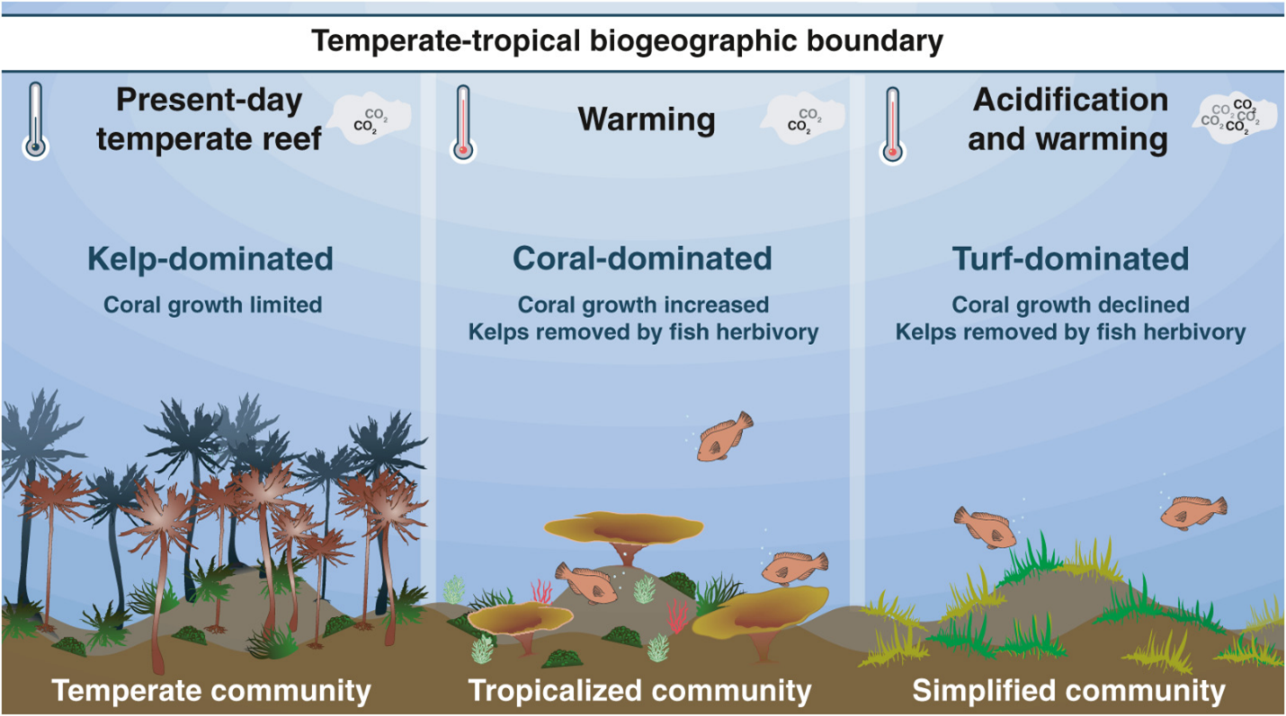
The altered species interactions caused by range shifts, life history changes, and other organism responses to climate change can have synergistic effects on ecosystems whose impacts are far greater than what we would predict by simply adding the impacts of each individual change together. Similarly, stressors such as ocean acidification, pollution, and poor fishery management can interact with climate change to drive feedbacks that result in abrupt and dramatic ecosystem changes that are far bigger than we would expect by simply looking at the effects of each stressor separately. The end result can be a sudden and radical shift in how ecosystems are structured, how they function, and the services they provide. In ecosystem jargon, such dramatic and persistent shifts are called regime shifts. Coral reefs provide an example. Tropical and temperate reefs have different appearances, reflecting the different ways their species interact and influence the flow of energy through them. Tropical reefs have lots of herbivorous fish that spend their days constantly grazing on algae. As a result, tropical reefs don’t have much large seaweed or kelp, but they do have lots of large and structurally complex coral that would otherwise get shaded out by the algae (see Fig. 3.2). In contrast, temperate reefs have lots of large, structurally complex kelp and seaweed, far fewer grazing herbivorous fish, and fewer structurally simpler coral.
This characteristic distinction between tropical and temperate reef regimes is beginning to break down as tropical species colonize temperate reefs. In some places, species interactions and feedbacks between stressors have caused rapid and dramatic shifts into entirely novel ecosystem regimes. For example, the coastal marine ecosystem of southwestern Australia is dominated by an extensive kelp forest that until a few years ago stretched from the town of Kalbarri southward along the coast for about 800 km. Over the past several decades, the waters off the coast of Western Australia have been rapidly warming, and that has caused the subtropical edge of the kelp forest to contract. After a particularly warm year in 2011, the kelp range contracted by 100 km. At the same time, tropical species have been expanding into the kelp. These include corals, invertebrates, and most notably numerous herbivorous fish. The tropical grazers reduce kelp cover in their own right and importantly prevent kelp from recovering after heat waves or other disturbances.41 Large stretches of what used to be kelp forest have been rather abruptly transformed into systems that more closely resemble tropical coral reefs.
Marine temperate ecosystems in other regions have become tropicalized in a similar way. But the transformation is messy. The new systems more often than not are hybrids that look a bit like tropical reefs in some respects and a bit like temperate reefs in others. We do not have a good understanding of how these new hybrid ecosystems function or how they differ in terms of the ecosystem services they provide. It is possible that tropicalization of temperate marine ecosystems could provide a measure of ecosystem resilience, helping them to maintain biodiversity and ecosystem functions in the face of climate change. That is far from certain, however. There is evidence that other factors such as ocean acidification or the loss of top predators from overfishing can interact with range shifts to further alter ecosystem structure. For example, some temperate reefs along the coast of Japan have become tropicalized by the expansion of tropical fish and coral species, resulting in hybrid reef ecosystems dominated by coral. In some areas, however, natural CO2 seeps have created unusually acidified water that seems to have inhibited the migration of coral species, resulting in significantly simplified ecosystems that support reduced biodiversity (Fig. 5.9). It’s clear that these highly simplified systems provide far fewer ecosystem services than either the original kelp system or the more fully tropicalized coral system. Even in cases where range shifts lead to increases in local biodiversity, it is still likely that the changes in species interactions will cause disruptions, at least to the particular suite of services that we are accustomed to.
Shifting Fisheries
Our disruption of marine ecosystems is troubling, especially because we depend on the ocean for a considerable part of our health, livelihood, and well-being. Marine ecosystems provide us with a broad range of goods and services such as climate regulation, storm protection, new materials and medicines, recreation, and tourism. Setting all that aside, just the fish we extract from the ocean provides 3 billion people with 15% of their animal protein, and getting that fish to them supports the livelihoods of about 8% of the world population.42 Although we know that marine ecosystems are changing, we are far from certain about how those changes will affect fisheries and the societies that depend on them. The impact partly depends on what emissions scenario we follow (see Section 4.5), but it also depends on the details of how ecosystems rearrange themselves. The more optimistic predictions suggest that the overall ability of marine ecosystems to support fisheries will not change much as climate warms. Instead, where those fisheries are located and the species they contain will shift. Under these predictions, fishery productivity is expected to increase in high latitudes and decrease in low to middle latitudes, but with a lot of variation within regions.43 Such shifts could be beneficial for some folks and regions. For example, the abundance of skipjack tuna (Katsuwonus pelamis) could increase in the eastern Pacific as climate warms through the century. The increase in abundance of this valuable fishery species could help offset the social impact caused by regional declines in coral reefs.44 But overall, the prospect of shifting fisheries is not something to look forward to. Our social and political structures are more fixed than the fish are. Many tropical regions such as Southeast Asia and the equatorial Pacific coast of South America are highly dependent on fisheries, and these are the same regions that are expected to see declines in their fisheries.45
Some communities, such as Isle de Jean Charles, are almost entirely dependent on marine resources. These communities are often the poorest and most marginalized among us, and they have the least capacity to adjust to a changing ocean. The fact that the fish they depend on for their livelihood may be abundant hundreds or thousands of miles away is of cold comfort. Nations contentiously fight over access to marine resources, and the compromises they make with each other often take the form of fixed boundaries on a map. For instance, under the United Nations Convention on the Law of the Sea, countries have exclusive rights to marine resources in a zone that extends 200 nautical miles from their coastlines. The fish, of course, don’t care about these boundaries, and countries still argue about how much fish each of them are taking out of the common ocean pool. Such disputes are likely to increase in frequency and intensity as fisheries rearrange themselves. For example, countries in the European Union that have mackerel (Scomber scombrus) fisheries have worked out a system of catch quotas in an effort to equitably share the resource. In recent decades, however, mackerel have colonized the warming waters off of Iceland. This has set of an Icelandic mackerel fishery boom. Icelandic fishers are not subject to the European quota system, and that has caused considerable exasperation among the Europeans.46
There are some reasons to be even more pessimistic. Many of our initial attempts to predict how climate change will affect fisheries have been necessarily simplified. Models often consider only how changes to thermal conditions will affect the geographic ranges of individual species. They also often focus on a single life stage, such as adults. But water temperature is just one aspect of a species’ niche. Climate change can also influence other niche components like pH or the availability of food sources. In addition, the different life stages of marine organisms often have different habitat requirements. Conditions that may be suitable for adults may be uninhabitable for juveniles. Models that incorporate some of that complexity often make more pessimistic predictions about the climate resilience of fisheries. For example, some of these more detailed models have been used to predict how climate change will affect commercially important tuna species in the North Pacific. The models suggest that climate change will increase the geographic displacement between areas that are thermally suitable for juveniles and areas suitable for adults. The increased displacement will force many tuna species to travel farther and spend more time in less optimal conditions. The warming waters will also increase metabolic demand for oxygen. As a result, many tuna species will need to eat more food to satisfy their increased metabolic requirements. At the same time, warming waters are expected to decrease food abundance for adult and juvenile tuna. One model predicts that under RCP 8.5, the combined effect of these stressors will reduce the carrying capacity of tuna species by 20% to 50% across the North Pacific by the end of the century.47
5.4 The Big Melt
Section 5.4: The Big Melt
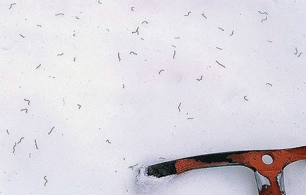
The cryosphere encompasses the parts of the planet that have frozen water. That includes ephemeral habitats such as seasonally frozen lakes and streams and even the snow cover that blankets many parts of the middle and high latitudes during winter. But most of the cryosphere is made up of habitats that are covered in snow and ice all year round. Places such as the massive Greenland and Antarctic ice sheets, the sea ice covering the Arctic Ocean and fringing Antarctica, and high-altitude glaciers. It also includes vast stretches of long-frozen soil in the high latitudes. In Chapter 4 I describe the role that the cryosphere plays in regulating Earth’s energy balance, driving climate feedbacks, and shaping the global pattern of wind and ocean currents. That gives the cryosphere an influence on ecosystems far distant from the polar ice caps or glacier-covered mountaintops. The cryosphere supports a unique collection of ecosystems in its own right. Cryosphere habitats don’t support many species; indeed, many parts of the cryosphere have conditions that are at the extreme limit of biological tolerances. The species they do support are exquisitely unique, however, such as the glacial ice worm (Mesenchytraeus solifugus) that lives its entire life on glaciers (Fig. 5.10). As you might suspect, the cryosphere is particularly sensitive to a warming planet. To put it simply, the ice is melting (See Fig. 4.8). In this section, I outline some of the main impacts that the melting is having on ecosystems.
The Availability of Fresh Water
Snow and ice play an important role in regulating the flow of fresh water through many terrestrial ecosystems. In high latitudes and regions with mountainous topography, seasonal snowmelt drives regular water cycles in soil, streams, and rivers. Climate change is altering both the timing and volume of these flows. Almost everywhere except the coldest parts of the cryosphere, warming over the past decades has reduced the amount of accumulated snow (measured in early spring) and hastened the onset of the snowmelt season.48 In many regions, this warming has shifted the timing of spring floods earlier. In northeastern North America, for example, the timing of spring high flows has gotten progressively earlier for most of the rivers over the past 90 years or so.49 A similar pattern has been observed for rivers in the western United States, and models predict that by 2050, peak spring stream flows in the region will occur about one month earlier if current warming trends continue. In many places, proportionally more precipitation is also falling as rain instead of snow, reducing the volume of spring and summer flows while increasing the volume of winter flows.50
Changes to snow- and ice-driven hydrology can have wide-ranging impacts on organisms and ecosystems, even ones distant from where the melting happens. Many species tune their life history to annual spring floods. For example, successful establishment of young cottonwood (Populus spp.) requires patches of bare riverbank and floodplain that are scoured out during the spring high-water season. Throughout much of the western United States, the frequency and intensity of these scouring floods have declined primarily because of dams. This has caused a long decline in cottonwood abundance along rivers such as the Green River in Utah. Further reductions in peak flows caused by climate change could contribute to even further cottonwood decline.51
Ecosystem processes such as primary production can also be altered by shifting hydrological regimes. Spring snowmelt and increasing light levels fuel a boom in the primary productivity of alpine streams, similar to the spring phytoplankton bloom in marine systems. Surging water from snowmelt supplies downstream aquatic plants and algae with nutrients at the same time that light levels are high. If the surge in water happens earlier in the year, however, the coincident timing of nutrients and light can get out of sync: the snowmelt-supplied nutrients arrive before light levels are high enough for plants to make full use of them. This happened in the alpine rivers of Austria during one particularly warm year in 2013-2014. That spring, primary productivity in the streams was significantly reduced, and the streams became net exporters of CO2 when previously they had been net sequesters of CO2. Also, less primary production was exported downstream to larger rivers and coastal waters.52 Even ecosystem processes seemingly far removed from the cryosphere can be influenced by changes in it. Models suggest that declining snowpack in the western United States could lead to increased fire risk in some places. With a smaller snowpack, soils dry out much quicker over the course of the growing season. This combined with projected warmer and drier summers will make the fuel available for a fire drier and more likely to burn increasing fire risk, at least in high-elevation forests where the flammability of fuel is a key predictor of fire risk.53
Mountain snowpack as well as longer-lived glacial systems provide massive freshwater storage that is slowly released to lower-elevation ecosystems and human communities. For example, meltwater from the Tibetan Plateau provides much of the water for the major river systems of South Asia, including the Indus, Ganges, Salween, Mekong, Yangtze, and Huang He.54 In many arid and seasonally dry regions, changes to the size of the snowpack and its timing of melting could exacerbate problems of water scarcity. For example, more than 75% of the water flowing through the main river basins that provide California with water comes from spring snowmelt. But just as important as the amount is the role snowpack plays in the timing of water delivery. Water scarcity is caused by a mismatch between supply and demand. California’s Mediterranean-type climate creates an inherently epic mismatch because most of the precipitation falls in winter, while most of the water demand (driven by agricultural irrigation) occurs in the summer. Snowpack helps narrow the gap by stretching out the delivery of winter precipitation over the snowmelt season. The design of California’s water storage and delivery system is integrated with the natural storage provided by snowpack. Under projected scenarios, however, the time gap between peak supply and peak demand will grow as a greater proportion of the annual precipitation falls as rain and snowmelt comes earlier. Existing reservoirs and groundwater storage facilities won’t be able to hold on to much of the earlier runoff because the storage facilities must maintain a storage buffer in order to provide their flood protection function.55
Rising Sea Level
As the ocean absorbed heat over the past century, it expanded, causing global mean sea level to rise. This expansion is still occurring as the planet warms, and it has been joined by another process: melting ice. For sea level, the ice that matters are the vast stores of it on land, principally in the Greenland and Antarctic ice sheets. In contrast to floating sea ice that has already displaced its volume in seawater, melting runoff from glaciers and ice sheets adds to ocean water just like a tap left on in a bathtub. Together, rising water temperature and melting ice increased global mean sea level by 21-24 cm between 1880 and the early twenty-first century, the fastest rate of increase in at least the past 2,800 years.56 Driven by increasing ice melting rates, that already rapid pace has increased in recent decades and is now at 3.4 mm per year. Just as with temperature, that global average blurs a lot of regional and local detail, and it also purposely removes the effect of changes in land elevation such as subsidence and tectonic uplift. But those details matter at the local scale. For example, while local relative sea level along the US Gulf Coast has been rising at nearly 12 mm per year (partly because of subsidence), it is actually decreasing in many places along the Gulf of Alaska where the landscape has been rebounding upward after the heavy ice sheets that once covered it receded.
The degree and pace of future sea level rise are two of the least understood physical processes related to climate change, primarily because we don’t really understand how the Greenland and Antarctic ice sheets will respond to rising temperature. Those parts of the cryosphere hold about 24,064,000 km3 of water, 1.7% of all the water on the planet. If all that water melted, it would raise global sea level by about 65m,57 radically altering the geography of the planet and among other things submerging most of the world’s coastal cities. We used to assume that it would be essentially impossible for human-driven climate change to melt the majority of that ice, and that even if we somehow could, the process would play out gradually over thousands of years. While it still seems extremely unlikely likely that we could melt all the ice in Antarctica and Greenland, we are no longer so certain that we can’t melt a significant chunk of it, or that that the melting will be slow and gradual. As we learn more about the dynamic life of the two ice sheets, they are beginning to look less stable than we had presumed. One factor is that the processes that influence melting involve feedbacks that can accelerate melting and push the ice sheets toward stability tipping points. One of these feedbacks is the melt-elevation feedback: melting reduces ice sheet height, which exposes more of the sheet to warmer temperatures at lower elevation, which accelerates further melting. There is evidence that this feedback has pushed at least one part of the Greenland ice sheet near a tipping point beyond which the region will be extremely susceptible to rapid melting. Comprehensive long-term observations across the entire ice sheet indicate that the amount of ice flowing off of Greenland through its glaciers dramatically increased at the start of the twenty-first century. The accelerating ice loss has now likely pushed the ice sheet into a state where it will be persistently losing ice for some time, even if we take action to limit future global warming.58
Another factor contributing to the instability of the ice sheets is topography. If the ice sheets were like blocks of ice sitting on a summer picnic table, they would melt gradually and predictably. But the ice sheets aren’t sitting on anything like a flat table. The Antarctic ice sheet is in a particularly precarious position. Much of its ice is perched into a giant, lopsided mound. In East Antarctica, the mound sits on continental land and is more than 4,000 m thick in places. In West Antarctica, the mound plunges 2,500 feet below sea level. All that ice doesn’t sit still; it slowly flows downhill into the Southern Ocean. We suspect that as things heat up, the ice will start to move faster, potentially in unpredictable and perhaps even catastrophic ways. You have experienced a similarly unpredictable system if you have ever made a pile of sand at the beach. As you add sand, the pile grows until suddenly and unpredictably a massive avalanche occurs on one or more sides. The same thing happens if you try to slowly take sand away or, potentially in the case of Antarctica, slowly melt ice. There is some evidence that the West Antarctic ice sheet is particularly susceptible to sudden collapse partly because it interacts extensively with relatively warm ocean water along its bottom; its collapse during the last interglacial period (129,000 to 116,000 years ago) was likely the major contributor to sea level being 6-9 m higher than it is today.59
Although there is still a lot of uncertainty, we have made considerable progress in recent years toward understanding the complex melting behavior of the Antarctic and Greenland ice sheets. The scientific consensus as of 2019 is that if we continue on our currently high greenhouse gas emission trajectory (RCP 8.5), global seal level will rise an average of 0.6 to 1.1 m by 2100, at an average pace of about 15 mm per year.60 By 2300, sea level could be as much as 5 m higher under the worst-case emissions scenario, although there is a lot of uncertainty in that estimate.
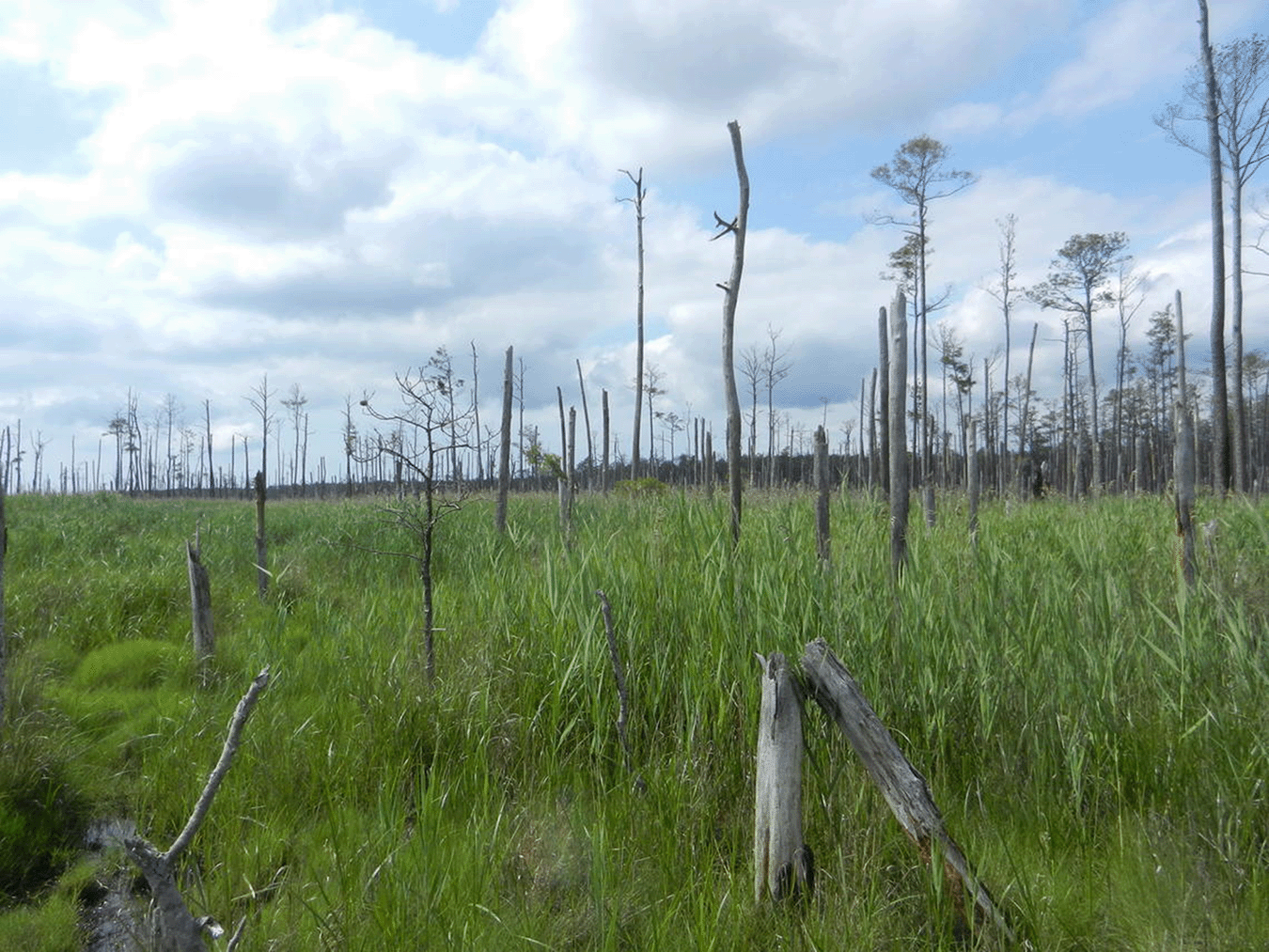
Rising sea level is changing coastal ecosystems such as estuaries, wetlands, and sandy beaches. An example comes from the freshwater wetland forests scattered along the coastal plain of the Atlantic and Gulf Coasts of North America. These forests occupy low areas that have chronically wet soils and that experience frequent (and often extended) periods of inundation. They contain species such as bald cypress (Taxodium distichum) that are adapted to a waterlogged life. While the species are well adapted to inundation, most are not well adapted to high salinity. The bottomland forests of the coastal plain tend to be found in areas that are set back from the immediate coastline, sometimes many miles away from the ocean. The water that usually inundates them comes from local rainfall or from rivers. Those rivers (along with groundwater) also hydrologically connect forests to the ocean. Historically, big storms such as hurricanes would rarely and sporadically push large surges of salt water inland. The unusual periods of saltwater inundation would severely stress bottomland forest trees and sometimes even kill large swaths of them. But such intrusions were rare, and the disturbances they caused were spatially limited and patchy.
Today, sea level rise is turning what used to be a rare and isolated event into a chronic widespread stress. First, higher sea level intensifies storm surge, which causes the saltwater flooding to affect a larger area and the inundation to last longer. Second, higher sea level drives a chronic and increasing push of seawater through the groundwater system even without the help of a storm. As a result, salty and brackish water is intruding farther inland, and bottomland trees are increasingly experiencing chronically high salinity. In many locations, the saltwater intrusion has created ghost forests of still-standing salt-killed trees (Fig. 5.11). Saltwater intrusion is driving a remarkably rapid loss of bottomland forests across the entire coastal plain of North America that stretches from southern Canada to southern Texas. Over a span of just 20 years between 1996 and 2016, the region lost 8% of its wetland forests, largely as a result of saltwater intrusion. Unless we alter the trajectory, we will lose these culturally and ecologically important forests altogether by the end of the century.61
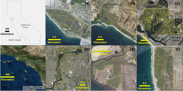
While rising sea level destroys habitat for some species, it creates habitat for others. In the case of the coastal plain of North America, wetland forests are being replaced by saltmarshes dominated by more salt-tolerant shrubs and forbs. One potential way that species and ecosystems could adjust to rising sea level is simply to move inland. On a topographic map, the wide and mostly flat landscape along the Atlantic and Gulf Coasts of North America seemingly provides a lot of space for species to spatially rearrange themselves. But the reality on the ground is a lot more challenging. An array of barriers such as farms, cities, and dams currently block wetland forests in most places from migrating inland. Around the world, coastal wetland species and ecosystems are getting squeezed by rising sea level on one side and human barriers on the other. The situation is particularly dire in regions with a high level of human activity and less forgiving topography, such as Southern California (Fig. 5.12). There is simply nowhere for many of the tidal wetlands in Southern California to go. One study estimated that if the high-end scenarios for sea level rise happen, all of the vegetated habitat at the Newport, Sweetwater, and Tijuana marshes (Fig. 5.12D–F) will be lost by 2110.62
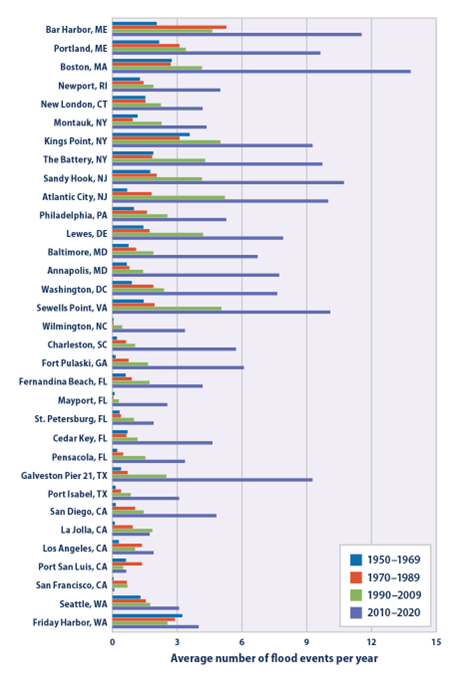
Rising sea level bodes ill for the roughly 10% of the world’s people that live in low-lying coastal areas.63 Higher sea level exacerbates the intensity of flooding and damage associated with extreme events like storms, and it increases the frequency of more run-of-the-mill flooding associated with high tides and mildly inclement weather. For many communities in the United States, the incidence of coastal flooding has increased significantly over the past several decades (Fig. 5.13). Our coastal infrastructure is also susceptible to saltwater intrusion via groundwater just like wetland forests are. The salt water can slowly corrode concrete and steel structures, cause sewer and septic tank failures, and contaminate drinking water sources.64 All of these impacts currently are and increasingly will be costly for our coastal communities. These costs include the direct human and economic costs from more intensive flooding, saltwater intrusion, and the loss of ecosystem services from habitats such as wetlands. The costs also come from our efforts to adapt to the new risks by improving flood protection, building more flood-resilient living spaces, and in many cases moving inland. The migration of people away from the coast will also stress the inland communities that take in the climate migrants.65
Disappearing Habitat
As the cryosphere warms, it is changing the way organisms interact with it. Not surprisingly, organisms that have the most highly developed adaptions to its extreme conditions are being stressed the most. They are like Formula One race cars that suddenly find themselves ferrying the kids to soccer practice through rush hour traffic. For instance, parts of the Southern Ocean never get warmer than a couple degrees above the freezing point of seawater. Many species that are endemic to the region die if temperatures rise just a few degrees above that narrowly cold temperature range. Many of the traits that allow species to survive extreme cold involve physiological trade-offs that reduce their ability to withstand even slightly warmer temperature. For example, some Antarctic fish and invertebrates lack heat shock proteins, which are almost universally present in other organisms. Heat shock proteins protect and repair damage to proteins from various forms of stress, notably high temperatures.66
Species that directly utilize ice are also particularly vulnerable. For instance, many species use sea ice as feeding or breeding platforms. Emperor penguins (Aptenodytes forsteri) breed almost exclusively on sea ice. Other regular ice users are marine mammals such as seals, walruses, and polar bears. Ringed seals (Phoca hispida), for instance, build lairs on the sea ice where they give birth and rear their pups. In turn, polar bears (Ursus maritimus) use sea ice as a platform to hunt their primary prey: seals. These species have life cycles that are finely tuned to the seasonal ebb and flow of sea ice. This habitat is quickly changing. The extent of arctic sea ice (measured at the end of summer) has been declining by about 13% per decade since good recordkeeping began in the late 1970s (see Fig. 4.8). The ice extent has also been receding more quickly in the spring and is taking longer to expand in the fall. We are just beginning to understand how changes in ice cover affect these marine mammals. Polar bears are a good example of our incomplete understanding. Their use of sea ice platforms is complex and varies considerably across their range, but many polar bear populations migrate onshore during the summer when the sea ice extent is low and it gets harder to move around on. For polar bear populations in the Canadian Arctic, the threshold sea ice cover is about 50%; when ice cover falls below 50%, bears migrate to land.67 There they spend the summer eating seabirds, scavenging, and pining for the sea ice return so that they can start eating fat, tasty seals again. The change in sea ice cover and timing has severely disrupted the lives of these polar bears, which now face extended periods scrounging for food instead of feasting on seals. For many polar bear populations, this has resulted in nutritional stress, declines in body condition, and reduced reproductive success.68 Based on the expectation that sea ice will continue to decline, polar bears were listed as a threatened species under the US Endangered Species Act in 2008, the first time a species had been proactively placed on the list in anticipation of future population declines.
Polar bears can adjust behaviorally to the rapidly changing conditions in the cryosphere by making greater use of alternative land-based resources such as ground-nesting seabirds. There is also evidence that they can rapidly adjust evolutionarily. Hybrids between polar bears and brown bears (U. arctos) have recently been observed (Fig. 5.14). The hybrids combine traits of both parents, which could be advantageous as climate shifts.69 Analysis of their genomes indicates that polar bears and brown bears commonly interbred and shared genetic information during the Pleistocene. That exchange of genes may have played an important role in helping both lineages survive that climactically tumultuous time.70 Still, it’s unclear whether these adjustments will be sufficient to keep the species from going extinct. We also don’t fully understand the broader ecosystem consequences that changes in polar bear life history could have. For example, polar bears have started to cause serious damage to nesting seabird populations in some locations, and the incidence of dangerous polar bear-human interactions has increased.71
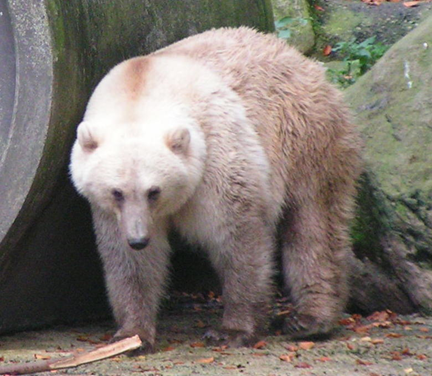
There is more to sea ice habitat than being a handy platform. It is a complex ecosystem unto itself that supports a diverse community of organisms far beyond marine mammals and nesting penguins.72 Sea ice has an intricate internal structure of brine-filled channels, which is the habitat for a diverse ice algae community that forms the base of the sea ice food chain. A diverse microbial community lives within the brine channels, feeding on the ice algae and their wastes. Zooplankton, including the juvenile stages of many benthic species, visit the brine channels to feed on the algae and other microbes. Specialized communities of fish and invertebrates are also closely associated with sea ice, and these in turn are key food sources for many seabird species. We do not understand how changing sea ice will influence this unique ecosystem, but we are beginning to see some impacts on individual species. For example, Ivory gulls (Pagophila eburnea) are highly dependent on sea ice, which is their primary feeding ground. Populations of Ivory gulls have declined along the southern periphery of their range, most likely because of declines in summer sea ice extent.73
Declines in snow and ice habitats can also have indirect effects on species. Changes to the timing of snow accumulation and melting can alter species phenology and cause trophic mismatches. For example, caribou (Rangifer tarandus) herds migrate to take advantage of seasonally ephemeral patches of high-quality forage. These feeding grounds are particularly important to calving success. In Greenland, warming has advanced the growth phenology of the plants in the caribou’s summer range, but the caribou haven’t kept pace with the shift in timing, so that they now arrive at their summer range after the peak in food abundance. This has increased juvenile mortality and reduced the reproductive success of the herd.74 Disruptions in timing can be particularly important for short-term summer visitors. Every summer in the Northern Hemisphere, red knots (Calidris canutus) travel from various winter homes scattered around the world to the arctic tundra to breed during the brief period when the Arctic has a superabundance of arthropod food. The red knot population that breeds in the high Canadian Arctic has one of the most epic migrations of any species, traveling nearly 15,000 km from Tierra del Fuego at the tip of South America. The red knot population that breeds on the Taimyr Peninsula in Russia accumulates fewer frequent flier miles, only traveling to and from the west coast of equatorial Africa.
The red knot migration is not as simple as hopping on an airplane. The birds carefully time their movements to follow the advance of spring across the temperate latitudes. But the Arctic is warming far more quickly than lower latitudes, and that has screwed up the red knot’s timing. Warming-related phenology changes have advanced the timing of the red knot migration through Europe by about 0.25 days per year over the past several decades, but that is only half the rate at which the timing of snowmelt is advancing farther north on the Taimyr Peninsula. As a result, red knots arrive on the Taimyr Peninsula out of sync with the phenology of their arthropod food, and their chicks now hatch after the peak arthropod abundance. This mismatch could be a significant reason for the recent steep decline in red knot populations although, interestingly, the nutritional effects of the mismatch don’t have a big impact on fitness until the birds are back in their tropical winter habitat.75
We are far from understanding what exactly will happen to the cryosphere as the ice melts. Like the polar bear, many cryosphere species can adjust. Behavioral adjustments, other forms of phenotypic plasticity such as physiological acclimatization, and evolutionary change (which can sometimes occur rapidly) can all help buffer the impact of declining ice habitat on individual species. In the medium term, a cryosphere that is a little less icy might be able to support a more diverse mix of cold- and warm-adapted species. But there will undoubtedly be individual losers and broader consequences to the changes.
5.5 Rearranged Landscape
Section 5.5: Rearranged Landscape
Many of the climate-driven changes occurring in the ocean and cryosphere have counterparts in ice-free terrestrial landscapes. There are some specific details that are unique to the changes occurring on land, not the least being that more of us live in and are intimately connected to the ecosystems that are changing.
Range Shifts
Terrestrial species are shifting their ranges generally poleward and higher in elevation, although at less than a quarter of the speed at which range shifts are occurring in the Ocean.76 One reason for the slower pace may be that the terrestrial landscape is generally more difficult for species to move around in than the marine world. Mountains, bodies of water, and human-constructed habitats such as cities and farms pose dispersal barriers for many species. A lot depends on the specific life history characteristics of individual species and how those interact with specific regional geography and microclimates. The ecological history of how plants in the Northern Hemisphere responded to climate change at the end of the Pleistocene provides a good example; 25,000 years ago, a massive ice sheet covered much of northern Europe, but as the glaciers retreated, plants began to recolonize. Some species quickly expanded their range into the newly emerged habitat. These species had traits that are commonly associated with early colonizing species: high dispersal ability (e.g., wind-dispersed seeds) and broad environmental tolerances. Many early colonists also had long-lived persistent seed banks, possibly because those species survived (even if only as seeds) in small ice-free areas that were isolated considerably farther north of the southern extent of the ice sheet. Once conditions started to improve, they got a head start on recolonization. But the early colonists were an exception. Many more species expanded their range north at a much slower pace. In fact, many European plant species currently occupy ranges that are just a fraction of the size they could potentially be based on current habitat suitability.77 It’s not clear why these species have been so slow to adjust.
We generally have a difficult time predicting how individual species will adjust their ranges in response to climate change. Range shifts seem to be a highly taxa-specific and contextual process. For example, climate change is causing the range of birds in Great Britain to shift north (by an average of more than 32 km over the past 40 years), but each species is taking its own idiosyncratic path north across the landscape. In part, this seems to be because each species is responding to its own climate cues. For one species, the critical driving factor might be temperature in late May; for another, it might be summer rainfall; for another still, it might be the amount of winter snowfall. The spatial patterns of these factors (and likely many more) are changing in complex ways across Great Britain.78 Trees in the eastern United States are making similar species-specific adjustments to their ranges. Overall, eastern tree species have been shifting their ranges north and west in response to climate change. Somewhat surprisingly, most species have been responding more to changes in precipitation than temperature, with most shifting west away from decreasing rainfall in the southeast and toward increasing rainfall in the central United States. But a range of other life history traits are also influencing the paths species are taking. For instance, wind-pollinated species have been moving predominately northward, while animal-pollinated species have been moving predominately westward. The reason for that difference isn’t clear.79
The often complex geography across landscapes also complicates how species move in response to climate change. In addition to acting as dispersal barriers, topographic features such as mountains or large bodies of water create microclimates that are different than the overall average climate in the region. The different microclimates also respond individually as overall climate changes; some change more rapidly and others more slowly than the regional climate as a whole. The more slowly changing areas can provide climate refugia that allow species to persist in a region even if climate conditions elsewhere become unsuitable. Mountains often act as climate refugia. Current examples are the Madrean Sky Island ranges of the southwestern United States and northwestern Mexico (Fig. 5.15). They get their name from the fact that they rise steeply from the desert floor, forming a series of microclimate islands that are dramatically different from the surrounding sea of lowland desert. During the Pleistocene, the entire region was cooler and wetter than it is today. But as regional climate changed, what used to be far more widespread habitats such as pine-oak woodland became compressed and restricted to the sky island climate refuges.80
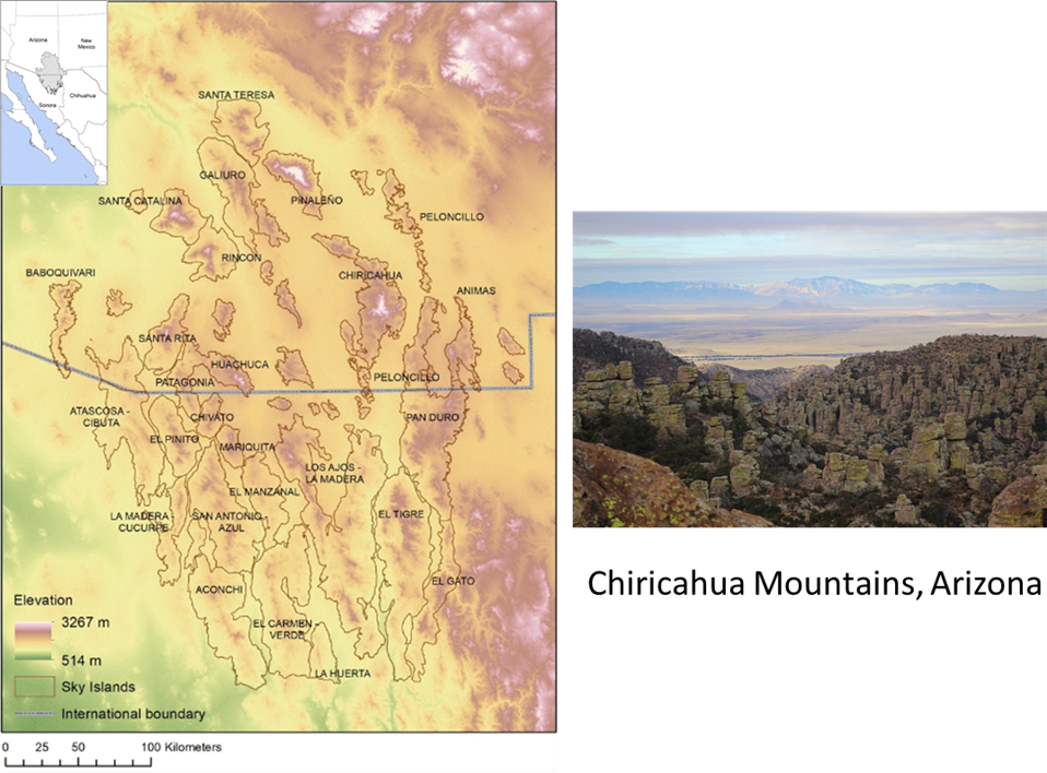
Although climate refugia provide a potential source of climate resilience, as a general rule, organisms will need to move considerable distances to find suitable climate. The pathways that many organisms will follow are called climate corridors. In simple terms, climate corridors are connected pathways of suitable habitat that organisms can disperse through. The tricky part is that these pathways don’t yet exist in the concrete way that the interstate highway system does. Instead, the pathways of suitable habitat will progressively develop as the microclimates that make up a landscape change in response to global climate. Instead of highways, climate corridors are more like paths of least climate resistance that organisms are likely to flow through as they get pushed away from deteriorating climate in one place and pulled toward improving climate someplace else. Where those paths of least resistance form and where they lead to depends on the details of local geography.
Mountains act as good climate corridors because they often provide the nearest source of suitable habitat as climate changes. Many species in mountainous regions have been shifting their range up in elevation as the microclimate at lower elevations becomes less suitable and the microclimate higher up becomes more suitable. In some regions, the move up in elevation connects to a network of favorable topography that could allow organisms to track hospitable climate across thousands of miles. The several north-south-oriented mountain ranges in North America are examples of potential continent-scale climate corridors (Fig. 5.16). Organisms could enter these corridors at the southern end by moving up in elevation, then following suitable habitat northward through the interconnected series of ridgelines, mountain passes, and valleys. In other regions, however, moving up in elevation leads to a dead end—a climate cul-de-sac.81 The Madrean Sky Islands fall into this category. Late Pleistocene organisms could easily move up the range, but once there, they had no easy dispersal pathway off, and they become trapped in an isolated climate refugia. In some respects, getting trapped wasn’t all bad. After all, being trapped is better than being extinct. Also, the isolation helped to generate new biodiversity. Many populations on the isolated sky islands began to evolve independently of each other and from other populations elsewhere in North America. Today, the Madrean ecoregion is a hot spot of biodiversity that contains many endemic populations of plants and animals. But sky islands and other climate refugia are like buildings with locked fire exits. Organisms have no escape route if something goes wrong. Anthropocene climate change is now threatening to push the unique sky island species off the tops of the mountains and into extinction.82
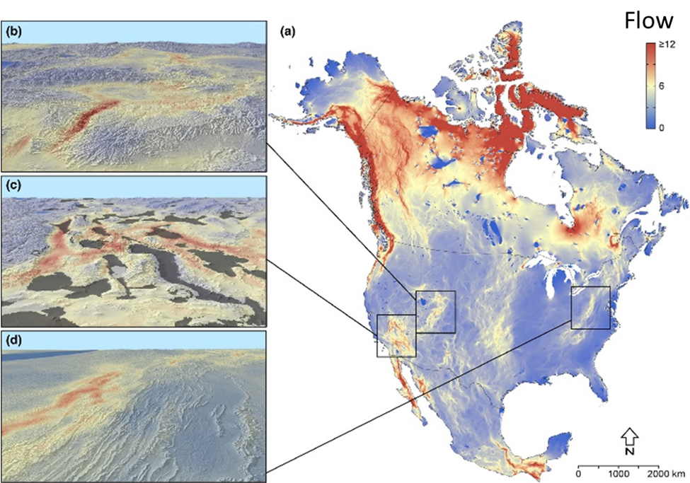
Gene Flow and Evolution
The Madrean Sky Islands illustrate that climate change can alter patterns of gene flow and influence evolution. Species exist as a network of subpopulations that are connected (to varying degrees) by dispersal. The aggregate web of populations is called a metapopulation. The subpopulations in a metapopulation commonly evolve adaptations to their specific location (see Fig. 2.6). For example, populations at the southern edge of a mammal’s range might be smaller or have less fur than those along the northern edge. In general, dispersal between subpopulations tends to mute these ecotypic differences by homogenizing genes across populations, while isolation and strong selection differences among populations tend to increase ecotypic differences.
This complicated structure can influence range shifts as well as the degree to which species respond evolutionarily to climate change. At an ecological scale, the individual subpopulations of a species might move at different rates or even in different directions depending on their local adaptations and climate conditions. At an evolutionary scale, gene flow (i.e., dispersal) between populations can distribute the genetic variability required for subpopulations to adapt to new climactic conditions. If local subpopulations can adapt, it might slow the rate of range shifts, for example, if cold-adapted populations along the northern edge of a range acquire warm-adapted genes from populations along the southern edge of the range.83
Researchers tested that hypothesis using a nifty experiment involving the Pacific Northwest annual wildflower Clarkia pulchella. The researchers first crossed C. pulchella individuals from northern populations with individuals from southern populations in a greenhouse. They then planted the resulting north-south hybrid offspring back out in the field along the northern edge of C. pulchella’s range and measured aspects of their fitness, such as survival and seed production. Individuals that were either the offspring of north-south crosses or were pure southern offspring had higher lifetime fitness than pure northern offspring. The result suggests that gene flow from southern populations could help northern populations persist longer at their current location and contribute adaptive genetic variation.84
Evolutionary changes can happen surprisingly quickly, and we are already seeing some evolutionary changes caused by climate change.85 The speed at which adaptations are developing is partly indicative of how strong a selective force climate change can be. An example comes from the pitcher plant mosquito (Wyeomyia smithii). Its range extends from the Gulf Coast of North America to northeastern Saskatchewan, overlapping with the range of its namesake, the purple pitcher plant (Sarracenia purpurea). The mosquito, like many other arthropods, uses day length as a cue to initiate diapause at the start of winter. This cue works because in the middle to high latitudes, shortening day length is closely associated with the end of the growing season and the start of winterlike conditions. The exact relationship varies with latitude (as well as altitude). At lower latitudes, cool temperatures don’t arrive until late in the year, when day length approaches its yearly minimum. At higher latitudes, cool temperatures arrive earlier, when day length is still relatively long. Correspondingly, the day length that triggers diapause is longer for northern mosquito populations and shorter for southern mosquito populations. As a result of climate change, however, the average frost-free growing season across the contiguous United States has lengthened by almost two weeks since the start of the twentieth century (see Fig. 4.13). That shift would have caused mosquitos to shut down for the winter too early, while there was still plenty more time left to lay eggs and pass on more genes to the next generation. But pitcher plant mosquitos have responded to that strong selective pressure by adaptively shifting toward shorter, more southern day-length cues, with northern mosquitos shifting the most. The shift has allowed the mosquitoes to stay synchronized with the lengthening growing season. Remarkably, changes in the mosquitos’ diapause timing have been observed to evolve in as few as five years.86
Climate change can also cause evolutionary change by fostering hybridization between previously distant populations. The periodic climate-driven encounters between polar bears and grizzlies (see Fig. 5.14) are a good example. In those cases, hybridization resulted in increased levels of genetic diversity that may have facilitated adaptive evolution. But hybridization can also homogenize what were once distinct gene pools, reducing overall levels of genetic diversity. For example, cutthroat trout (Oncorhynchus clarkii) and rainbow trout (O. mykiss) are found in streams and rivers across much of the western United States. Historically, their different habitat requirements and geographic ranges meant that individuals of the two species rarely encountered each other. But in recent years, we have increasingly caused their paths to cross. First, we introduced rainbow trout into river systems that were previously solely the range of cutthroat trout. In many of these systems, the newly arrived rainbow trout have hybridized with cutthroat trout. This has already caused two unique cutthroat trout subspecies to go genetically extinct, and many other unique subspecies are threatened. Some river systems have historically provided a refuge for cutthroat trout because they were environmentally unsuitable for rainbow trout. Rainbow trout prefer warmer streams that experience earlier spring runoff and lower spring flows compared to the conditions preferred by cutthroat trout. The Flathead River system that straddles the Canadian-US border had been one of these cutthroat trout refuges. But climate change has allowed rainbow trout to expand their range up the river system, where they now widely hybridize with cutthroats.87
Changed Biodiversity Patterns
The examples above illustrate how climate-change-induced effects on gene flow and selection can alter biodiversity patterns. We view these changes across all three classes of biodiversity (genetic, functional, ecosystem) and through the lens of different metrics and scales (see Fig. 2.2). Climate change can affect the various aspects of biodiversity differently. In the case of C. pulchella described above, gene flow from southern populations will likely increase levels of genetic diversity among northern populations, but at the same time, it could make northern and southern populations genetically and functionally more similar, homogenizing genetic structure and functional variation at the scale of the species as a whole. Time adds another dimension of complexity. In the case of the Madrean Sky Islands, the warming that marked the end of the Pleistocene spurred an increase in genetic and habitat diversity when viewed from a regional perspective. The proximity of so many unique habitats and endemic populations make the region a favorite spot for naturalists today. But ongoing warming through the Anthropocene now threatens much of that diversity with homogenization and extinction.
Amid all this complexity, a few general patterns are emerging. One is that climate migrants tend to augment local genetic diversity (alleles and species) when they arrive, at least initially. As a result, local allele and species richness has tended to increase in the places receiving climate migrants such as locations at higher latitudes and elevations. At larger spatial scales, however, all the movement of organisms among geographic regions is making the regions more similar to each other in terms of the plants and animals they support.88 As described above, that pattern is also being observed in the ocean. British birds provide a specific terrestrial example. A sedentary British bird-watcher now sees more types of birds in their local area than they used to. From 1994 to 2006, the local bird species richness at any given spot in Britain increased, with the greatest increase happening in upland habitats. The increase was driven primarily by new migrants from warmer regions. These migrants tend to be habitat generalists that can be found throughout Europe. Bird-watchers with more wanderlust now see a bit less variety as they travel from spot to spot, and they more frequently encounter the same old generalist species.89
Mountainous regions are hot spots for these changes because they provide climate refugia and corridors for all the organisms on the move. In Quebec, Canada, for example, low-elevation species such as sugar maple (Acer saccharum) have been moving up in elevation at a rate of about 9 m per decade. The new arrivals have increased the local species richness at high-elevation sites by about 25%.90 The picture is a bit more complicated than just adding species to the local community. While some species are arriving, others are leaving by shifting their ranges farther up in elevation or by going regionally extinct. While the net result is an overall increase in local species richness, the composition of the species making up the community is different. Unfortunately, we don’t have a comprehensive picture of how these changes are unfolding across the world’s mountains. We do have a growing collection of studies that have focused on different groups of organisms in specific mountain areas (Fig. 5.17). In aggregate, the studies suggest that mountainous regions around the world have been rapidly accumulating new species and losing old ones. The average rate of species turnover is 12% per decade.91 That’s incredibly fast. The absolute magnitude of species turnover is roughly comparable to the level of species turnover seen during previous periods of recent climate change, such as during the Pleistocene, but those past changes played out over thousands of years, not decades. There is also a rough balance between arrivals and departures. That indicates that the species composition of mountain communities is radically changing. It’s not like the band is still together with just the addition of a new trombone player. The band has broken up, and everyone has gone off to explore new opportunities.
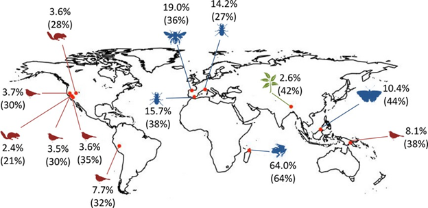
The novelty of these new species combinations is easier to see if we look at functional diversity. Any fan of fruit-eating (frugivourous) birds should visit the Manú biosphere reserve in the Peruvian Andes. There are at least 232 species of them there, although you have to take a walk uphill to see them all. Some of the species are lowland specialists, many are found at mid-elevation, and some are highland specialists. Each species differs in the types of fruit they eat and how they go about doing it. These functional differences are reflected in physical traits such as bill width and bill length. Researchers constructed environmental niche models for each of the species and used them to predict how their elevation ranges would shift under climate change scenarios.92 As expected, they found that climate change will drive a lot of species turnover across the elevation gradient as species generally shift their ranges uphill. Figure 5.18 depicts these changes in terms of functional richness instead of species richness.
The lowlands are expected to lose many functional groups, particularly birds that are specialized on eating large fruit such as the Razor-billed Curassow (Mitu tuberosum) and the Ivory-billed Aracari (Pteroglossus castanotis, P. azara). The loss of these big-fruit specialists could reduce seed dispersal of the plant species they feed on. Adjacent mid-elevations are expected to gain functional groups from the lowlands. The arrival of these novel functions could create radically new relationships and ecosystem characteristics, but we don’t really know how things will play out. Surprisingly, the functional composition at higher elevations is expected to stay about the same even though species turnover will be high and some high-elevation specialists are likely to go regionally extinct. The reason is that there is a lot of functional redundancy among the species across a broad-elevation range, so even if a particular species moves up in elevation or goes extinct, it will likely get replaced by a lower-elevation migrant with a similar function.
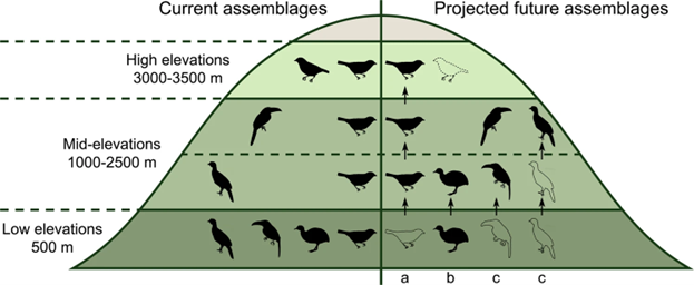
Altered Relationships
Not surprisingly, when species get thrown together as a result of climate change, they form novel ecological relationships. These new interactions can themselves influence biodiversity patterns and alter ecosystem functions and services. Ecosystem-scale effects are often most pronounced when the newly arriving species possess functional traits that are novel or rare in their new homes. The regime shifts caused by the poleward spread of tropical herbivore fishes described above are examples (see Fig. 5.9). A similar situation could be taking place in mountainous regions on land.
High-elevation plants generally experience less herbivory than lowland plants, and as a result they have evolved fewer defenses against herbivores (e.g., chemical defenses) than lowland plants. But climate change is shifting the ranges of lowland insects upslope at a much faster rate than those of plants.93 Poorly defended alpine plants could face an onslaught of novel herbivorous insects in much the same way that temperate reefs are dealing with the arrival of tropical herbivorous fish. An experiment conducted in the Swiss Alps provides some clues as to what might happen to alpine ecosystems as a result.94 The researchers used environmental niche models to estimate that high-elevation sites in their study area could experience a twofold increase in herbivore richness and more than a threefold increase in herbivore abundance by 2080. The researchers then experimentally simulated those conditions by translocating assemblages of grasshopper species (orthopterans) from a lower elevation into experimental cages established above the tree line in alpine grassland. They also simulated predicted warming using open chambers like those used in the SPRUCE experiment (see Fig. 5.6). In contrast to the dramatic loss of macroalgae species that tropical herbivore fish cause on temperate reefs, the translocated grasshoppers actually increased alpine plant species richness by 8.6%. The grasshoppers did this because they preferentially fed on species that resembled their preferred food back in the lowlands in terms of traits such as leaf toughness and leaf chemistry. The grasshopper-preferred species also happened to be the tallest, most structurally dominant species in the grassland. Grasshoppers reduced the biomass of the competitive dominants, resulting in a more open canopy that allowed shorter and less competitive species to establish and coexist with the dominant species. The results from this simplified experimental setup may not fully describe dynamics under more realistic conditions. It seems likely that at least under some circumstances, the arrival of lowland herbivores could lead to the loss of some alpine plant specialists or even general declines in plant diversity.
A perhaps even better example of how the arrival of novel functional traits can trigger a cascade of ecosystem changes is the expansion of shrubs into the high Arctic.95 The extreme cold temperatures and extensive permafrost of the high Arctic support a tundra vegetation that consists mostly of low-growing herbaceous plants and prostrate shrubs. But as conditions have warmed, taller woody shrubs from lower-latitude boreal ecosystems such as birch (Betula spp.), willow (Salix spp.), and alder (Alnus spp.) have expanded into the tundra. Just like algal forests in the marine environment, the presence of the shrubs creates a range of new ecological interactions partly because they are strong ecosystem engineers that modify abiotic conditions. In the winter, they trap insulating snow so that soil temperature under them can be up to 30°C warmer than air temperature. In the spring, their dark color reduces albedo and can speed rates of snowmelt. The changes in temperature patterns as well as inputs of leaf litter can alter biogeochemical nutrient cycles in complex and poorly understood ways. The tall shrubs are strong competitors for light and other resources, causing declines in herbaceous plant species such as moss and lichen that are important food for many species, including reindeer (Rangifer tarandus).96 At the same time, the shrubs provide forage and cover from predators for a range of other animals such as willow ptarmigan (Lagopus spp., L. muta), snowshoe hares (Lepus americanus), and moose (Alces alces) that have increased their abundance and expanded their range further into the tundra.97
Just as in the ocean and cryosphere, differential changes in phenology are creating mismatches in species interactions. Examples include emerging phenology-driven trophic mismatches between caterpillars and the host plants they feed on, between migratory birds and the caterpillars they feed on, between owls and their small mammal prey, and between freshwater diatoms and the water fleas (Daphnia spp.) that feed on them.98 In terrestrial habitats, one of the most important relationships is between plants and pollinators. It is likely that the warming climate is causing a widespread disruption of this key mutualism both by driving phenological mismatches between plants and their pollinators and by driving differential range shifts.99 The predicted climate-driven spatial mismatch between Mexican long-nosed bats and the agave species they pollinate described above is one example (see Fig. 5.6). We have some empirical evidence that climate change is already disrupting plant-pollinator relationships, although documenting these disruptions is challenging. An example of our still incomplete picture comes from a remarkable data set compiled by the entomologist Charles Robertson. Over several years in the late 1880s, he documented nearly all the insect visitors to flowering plants near his home in Carlinville, Illinois, USA. The resulting book, Flowers and Insects,100 is still one of the most comprehensive descriptions of plant-insect relationships for a single location ever done.
By resurveying Carlinville, subsequent researchers have been able to track how plant-insect relationships have changed, at least for the bees, which is the group the subsequent researchers focused on. By the early twenty-first century, the interactions between the bees and plants of Carlinville looked very different. Only 24% of the bee-plant interactions (i.e., a particular bee species visiting a particular plant species) that Robertson had observed still existed. Several new interactions had developed, but overall, there was a net loss of nearly half the interactions. This was partly because half of the bee species that Robertson had observed were no longer locally present; about 45% of the lost interactions were a result of the locally extirpated bees, most of which were specialists that visited only a few plant species.
Many of the local extirpations were likely the result of changes to the landscape around Carlinville, which has become less forested and patchier since the late 1880s. But climate change has likely also played a role, both by shifting the range of some bee species and by creating phenological mismatches. Compared to estimates made from Robertson’s data, peak flower bloom in 2009-2010 occurred 9.5 days earlier, while peak bee activity occurred 11 days earlier. A similar mismatch between plants and bees was seen in the overall length of bloom period (8 days shorter) and bee activity (22.5 days shorter). Statistical modeling of the data suggests that up to half of the observed changes in the bee-plant interaction web could be the result of phenological mismatches.101
Climate change can also drive evolutionary adaptations that in turn alter community interactions. In the alpine meadows of the Rocky Mountains, long-tongued bumble bee species have coevolved to pollinate plants that possess elongated corolla tubes. This is a mutualistic relationship: the plants are more effectively pollinated by a specialist group of bees, and the bees get access to an exclusive nectar resource that shorter-tonged bees can’t reach. Climate change has thrown the effectiveness of this intricate relationship out the window. Summer temperatures in alpine habitats around the world have been rapidly increasing. Initially, warming temperatures increase alpine flower abundance, but if temperatures continue to warm past a certain threshold, flower abundance declines. This happens partly because the warm conditions dry out soils more quickly in the summer, shortening the period when flowers are available.
This has been happening in the Rocky Mountains, where warm summers have significantly decreased the flower abundance in alpine habitats over the past 40 years. In response, the two most common bumble bee species (Bombus balteatus and B. sylvicola) have rapidly evolved shorter tongues. With overall fewer flowers around, it is no longer advantageous for bumblebees to specialize on the fraction of flowers with long corolla tubes. The shorter tongues allow the previous specialists to broaden the flower types they can feed on, compensating for the overall reduced flower abundance.102 This rapid evolutionary shift may allow these species to keep pace with climate change. While reassuring, it also brings up a range of other questions. Will other long tonged bee species be able to adjust? What happens to all the plants with long corolla tubes? Will competition increase between short-tongued bees? In the future, will there be a broad trend across all ecosystems for biological communities to be dominated be generalists with few unique specialists?
Diseases and Pests
Many of the relationships between organisms end badly for one of the partners. We understandably spend a lot of time thinking about the interactions that end badly for us: the pests and diseases that negatively affect our crops, other species we care about, and ourselves. Climate change can potentially alter the prevalence and severity of pests and diseases. One way is by facilitating the spread of organisms into new areas. Species that we consider to be agricultural pests or pathogens have been shifting their range poleward at an average rate of 2.7 km per year since 1960.103 This is faster than the mean poleward advance of 17 km per decade observed across all terrestrial taxa (for which data are available). Pests and pathogens might be shifting faster because they have evolved effective dispersal mechanisms and because we unwittingly assist their spread around the world through our movements and trade.
For many pests, dispersing or getting moved to a new location is not a problem. Instead, climate is the primary barrier that prevents a pest or pathogen from establishing in a new area. As with species in general, the arrival of new pests or pathogens can potentially trigger widespread ecosystem changes that can create particularly dramatic outbreaks or severe impacts. In addition, our human communities are often ill prepared to manage the new arrival or cope with the impacts. For example, during warm years in Ethiopia and Columbia, the mosquito vectors of malaria (Anopheles spp.) are found at higher elevations, exposing the people living there to an increased risk of contracting the disease.
Warm years happen occasionally as a result of natural variation, but their frequency has been increasing with climate change. In both countries, the number of new high-elevation malaria cases has increased over the past several decades. In Ethiopia, where a large proportion of the population lives at high elevation, a one-degree Celsius increase in temperature over conditions at the start of this century is expected to result in 2.8 million more infections among young people (<15 years) who are the most susceptible to infection.104 The risk of malaria as well as other mosquito-borne diseases such as yellow fever, dengue, and Zika is increasing globally as mosquitoes expand their range into previously inhospitable regions and the transmission season lengthens in areas where they are already present.105
Climate change could also shift the spatial pattern of disease risk. For instance, one of the main mosquitos that transmits malaria Anopheles gambiae has a different thermal niche than Aedes aegypti, one of the main vectors of several viral diseases such as dengue fever. Malaria transmission by A. gambiae peaks at 25°C, whereas dengue transmission by A. aegypti peaks at 29°C. Both mosquitoes are present across most of sub-Saharan Africa as are the diseases they transmit. But in many places, limited public health resources are focused on the most salient risk, which is often considered to be malaria. Climate change is expected to shift the spatial pattern of malaria and dengue risk in different ways (Fig. 5.19). Public health infrastructure and disease surveillance programs will need to adjust to the shifting risks.106
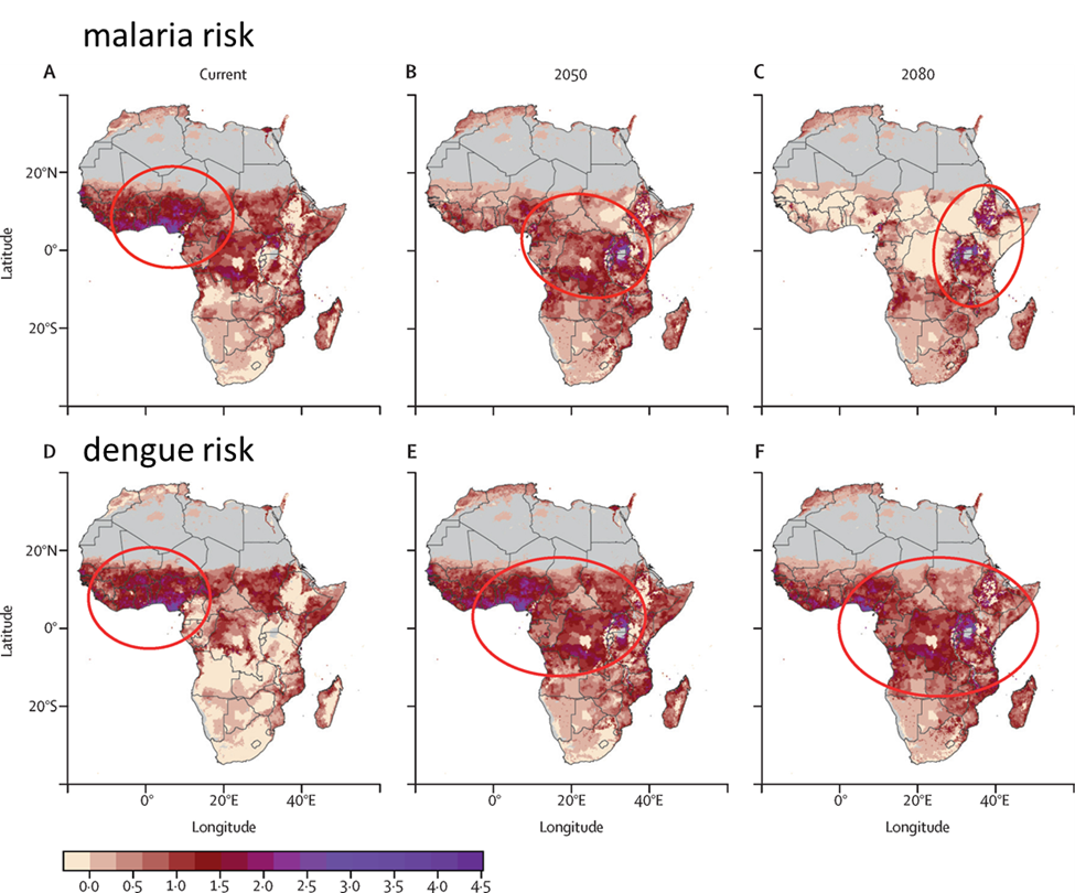
Range shifts that cause the arrival of a new pest are straightforward to understand, but climate change can also disrupt the relationship between pests and their hosts in bewilderingly complex ways. This makes it difficult to come to broad generalizations and predictions about the consequences. Exemplary of this complexity are the factors that regulate the interaction between plants, the insects that eat them, and the predators that consume (in one way or another) the insect herbivores. We have fairly robust evidence that rising temperature as well as atmospheric CO2 will spur plant growth—recall from Chapter 4 that the CO2 fertilization effect is one of the powerful climate feedbacks. But rising temperature also tends to increase the metabolism, feeding rate, individual growth rate, overwintering survival, and population growth of herbivorous insects. There is some evidence that this climate-driven acceleration of insect life cycles has caused pest outbreaks, particularly at high elevations and high latitudes. For instance, outbreaks of spruce beetles (Dendroctonus rufipennis) and mountain pine beetles (Dendroctonus ponderosae) in western North America have been linked to warming temperatures that increased the number of their annual broods.107 In addition, the CO2-induced spurt in plant growth tends to be higher in carbon and lower in nitrogen, making it less nutritious—sort of the insect equivalent of a high-carb diet. In laboratory experiments, the insects compensate for the reduced nutrition by eating more. For these reasons, it is possible that as CO2 accumulates and climate warms, overall herbivory rates will increase, at least at high latitudes and elevations. Indeed, the strength of insect herbivory generally declines as you move poleward, so it seems reasonable to expect that as regions become more tropicalized, herbivory will increase.
There is one other significant biological player in this grand interaction, however: the predators and parasitoids that consume herbivorous insects. Many of these are insects that will likely respond to a warming climate in the same positive ways that many herbivores will. This could suppress any increase in herbivores or even cause a trophic cascade that increases plant growth. A potential example of these interactions comes from the subarctic forests of northwestern Russia. From 1993 to 2014, spring and fall temperatures increased in the region by 2.5°C to 3°C, but contrary to expectations, the abundance of herbivorous leaf beetles did not increase; in fact, the densities of two of the four species of leaf beetle declined. These declines were partly the result of increased parasitism and predation rates on the leaf beetles. Some of the increased predation and parasitism seems to be related to climate change. But there is uncertainty in that interpretation because there was a heavily polluting smelter in the study that stopped operating partway through the study period. The end of smelter pollution could also have benefitted the predators and parasitoids.108
The idiosyncratic ways that species respond to climate change makes it even more difficult to predict how species interactions will change. An example comes from the insect pests of soybean (Glycine max). Early in the year, soybean plants are tolerant of herbivory so that even relatively high abundances of insect herbivores do not cause substantial reductions in yield. But things become more critical later in the year when the soybeans set flowers and the fruit starts to develop. Herbivory during these stages can cause severe reductions in yield. The difference is seen in the impact caused by two introduced pests to the US Midwest. Japanese beetles (Popillia japonica) cause a lot of damage to soybean leaves, but because the damage happens early in the year, it has only a minor impact on yield. The soybean aphid (Aphis glycines) tends to cause greater yield reductions, however, because its herbivory comes later, during the reproductive stages of soybean. Climate change that shifted the phenology of the soybean aphid and other later-season herbivores earlier relative to that of soybeans would reduce their impact.109
Agricultural Productivity
All of the disruptions to ecosystems discussed so far (behavioral and physiological adjustments, range shifts, evolutionary changes, changed species interactions, and altered biodiversity patterns) affect the services that we derive from them. But understanding how climate change will affect ecosystem services is one of the most difficult aspects of climate change science. Maddeningly, it is the aspect of climate change that we are the most uncertain about. A great example is food.
Food is one of the most fundamental services we get from ecosystems. We have a lot of interest in understanding how climate change is altering our ability to produce food and what the challenges could be in the future if we don’t significantly alter our climate trajectory.
One approach that we have taken is to evaluate the physiological responses of our principal food crops, such as wheat. The winter wheat study described in Section 5.2 is a good example. That case illustrates that climate change could have both positive and negative impacts for the physiology and growth of our crops. On the positive side, the CO2 fertilization effect could be a benefit. In greenhouse and small-mesocosm experiments, CO2 enrichment as well as elevated temperature increase yields of a variety of crop species.110 Longer growing seasons could also increase yield by allowing more crop harvests within a season as well as making some regions (particularly in high elevations and latitudes) more conducive to agriculture. Some regions might experience increased rainfall that could help to increase agricultural production. Counterbalancing these positive effects are negative ones. Higher temperatures could cause thermal and water stress. Many regions will receive less rain, or the seasonal patterns of rainfall will change. An increased frequency of extreme weather events such as intense storms, floods, and droughts could reduce average yields.
The available evidence from field studies and environmental niche models conducted for a few major crops (e.g., maize, wheat, rice, and soybeans) suggests that on balance the negatives will tend to outweigh the positives. There are distinct regional differences in the stress that crops will face, however. In general, crops in equatorial regions will be under much more stress than those at higher latitudes. For instance, under RCP 8.5, maize yields are expected decline by around 50% by the end of the century across much of the tropics, but they are expected to increase in many high-latitude regions.111
Just looking at the physiological responses of crop species doesn’t provide a complete picture. A number of other factors associated with changing climate can influence crop yields indirectly or affect our general ability to manage agricultural systems. One of these factors is the impact of pests and diseases on our crops. On average, pests and diseases currently reduce yields of our major crops by roughly one-third, with insects alone reducing yields by roughly 10%.112 But things could get worse under climate change. As described above, we know that as temperatures rise, insects eat more to support their rising metabolism, and they also experience increased population growth. Based on these basic physiological responses, insect-caused losses of wheat, rice, and maize could increase by 10% to 25% per degree Celsius of warming, with the biggest losses occurring in the temperate zone.113 Weeds could also get a similar physiological boost from climate change from warmer temperatures and CO2 fertilization. For instance, experimental warming and enhanced CO2 significantly increase the annual growth of several species that are widespread weeds in temperate cropping systems.114
Climate-change-driven range shifts could also expose crops to new pests and pathogens as well as increase the overall biodiversity of the pests that crops in a region are exposed to.115 But we have a poor understanding of how these potential changes will play out. Just as with crop species, climate change could affect pest species in negative as well as positive ways. From the standpoint of our crops, what we really want to know is how the individual responses will interact. The conditions promoting increased weed growth could also promote increased crop growth so that the net impact on yield is a wash. As with the soybean pest example above, subtle changes to the relative phenology of crops and pests can result in big changes to the resulting pest impacts. All these responses and their interactions are highly species and location specific. For instance, the expected climate change effects on the prominent pathogens of our four main crops (wheat, rice, soybean, and potato) are variable. Under climate change scenarios, some disease risks will likely increase, others decrease, and others will not change.116
Another important factor is pollination. Animal pollinators are either required for or enhance the yields of 75% of the 115 major crop species. Moreover, the fruit and vegetable crops that are most dependent on animal pollinators provide the majority of the world’s micronutrients such as vitamins A, C, and B, lycopene and a range of antioxidants.117 The climate disruptions to pollination networks described above could therefore have a severe impact on our nutrition and food security. But again, predicting what the net effect of the changes will be is not straightforward. Our crops are pollinated by managed populations of honeybees as well as from a diverse range of wild pollinators. In the United States, honeybees and wild pollinators provide about equal amounts of crop pollination, even in the most agriculturally intensive areas.118 An example of the diverse network of crop pollinators comes from the bees pollinating watermelon in the eastern United States. An assemblage of seven wild bee species pollinate watermelon in the region. In addition, farmers augment wild pollination by renting hives of European honeybees. Not all the species are equal when it comes to pollinating watermelon. Some are efficient at depositing pollen on watermelon stigmas, while others are pretty sloppy about it. They also vary in the amount of time they spend foraging in the watermelon. Differences in foraging activity are mostly driven by differential responses to temperature: some species have a narrow temperature range at which they are active, while others have a broader range. Researchers used the temperature-pollination responses for each of the species to predict what the net effect on overall crop pollination would be if temperatures increased.119 Assuming a pessimistic emissions scenario, they found that rising temperatures could cause a 14.5% reduction in the pollination service provided by managed honeybees by the end of the century. But rising temperature tended to increase the pollination activity of most of the wild bees so that in aggregate, overall pollination services could actually increase by 4.5% by the end of the century. It appears that having a diverse assemblage of crop pollinators provides a measure of climate change resilience.
The watermelon pollination study only considered the effect of rising temperature on the activity of bees, however. Other aspects of bee biology and health such as growth or phenology could also be altered by climate change. Also, other climate variables such as rainfall or the frequency of extreme events could have more negative effects than temperature. On a broader level, climate change is just one aspect of the Anthropocene. A wide range of other factors such as the heavy use of pesticides, other pollutants, landscape changes, and the spread of introduced diseases and pests have caused the overall abundance and diversity of pollinators to decline in recent decades.120 We are far from certain how all these things will combine in the future. The overall declines in bees, and our uncertainty about their future, is particularly troubling given how few species we rely on for pollination services in the first place. Even the wild pollinators of our crops consist of only a few common species that are a small fraction of overall pollinator diversity.121 Are these handful of species enough insurance for the coming changes?
We could alter farming practices in ways that support high levels of pollinator diversity (see Chap. 7). We could also adjust our agroecosystems in a number of other ways in an effort to adapt them to changing climate. How effective our adaptation strategies will be adds another layer of uncertainty in predicting climate change impacts. An important adaptation strategy could be the use of irrigation. Irrigation gives farmers a measure of control over when and how much water their crops receive that is somewhat independent of the vagaries of weather and even the longer-term constraints of climate. Its management value is reflected in how widespread it has become. In 2005, irrigated crops accounted for about 40% of global crop production and 70% of the fresh water we consume.122 There is some potential to increase that use even more as a climate adaptation strategy. One study estimated that under conditions prevailing in a world that is 3°C warmer than preindustrial levels, irrigation could be used as an adaptation strategy on up to 35% of currently rain-fed croplands.123 Those estimates were calculated using a requirement that the new irrigation does not negatively affect the water availability required to support other parts of the ecosystem such as fish. The authors also argue that expanding irrigation does not necessarily need to involve large infrastructure investments such as dams. But there are reasons to be skeptical that expanding irrigation could provide a net benefit at the global scale. As described above and in Chapter 4, changes to the cryosphere, shifting precipitation patterns, and the increased frequency and intensity of droughts will also significantly increase water scarcity in many regions that are currently dependent on irrigation. Increased water scarcity caused by climate change will likely make food costlier to produce, exacerbate water use conflicts, and in some cases make regions inhospitable for crop production.124
Another adaptation strategy is to shift what types of crops we grow. In many cases, as a region becomes climactically less suitable for some crops, it will become more suitable for others. Farmers are already doing this. From 1973 to 2012, the geographic growing ranges of rain-fed maize, wheat, rice, and soybean have shifted in ways that track their optimal climate requirements (Fig. 5.20). Wheat, maize, and rice production have all generally shifted away from regions with rising temperature stress to cooler regions. Soybean production is the exception. It has expanded into warmer regions, partly assisted by the development of new varieties. These changes are analogous to climate driven species range shifts.
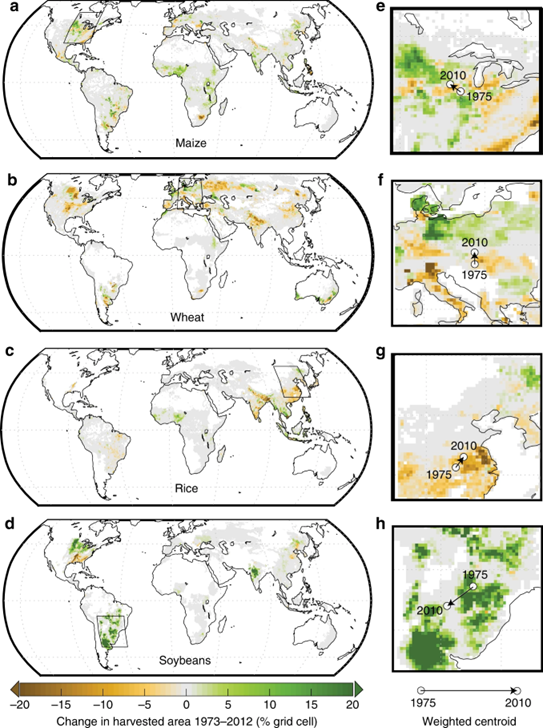
As is the case with fisheries, farmers often have limited capacity to adapt to climate change. Switching crops is not as easy as changing a seed order. It usually involves buying new equipment, learning new approaches, and finding new markets. Crop switching and the other adaptation strategies require significant financial investments as well as access to a range of other resources such as credit, information, and locally relevant applied research such as breeding programs. Poor farmers as well as communities that are already the most food insecure have the least capacity to adapt and face the most risk from climate change.125
All that complexity and contingencies make it difficult to predict what the future will hold. But we can also look at the impact climate change has already caused. Using the approaches described in Section 4.4, researchers can now estimate what fraction of the weird weather that a region experiences is attributable to climate change. They can then correlate how observed crop yields have been affected by climate-change-related weather extremes such as prolonged droughts or unseasonably warm temperatures. Researchers used that approach to estimate how climate change altered the global yields of our top 10 crops from 1974 to 2008.126 They found that climate change over that time caused widespread reductions in yields, even in regions that presumably have relatively high capacity to adapt. For instance, yields in Europe declined 6.3% to 21.2%. Some other regions have fared better; yields in most of Latin America actually benefitted from climate change. But overall, the yield declines have translated into less food. We lost about 1% (-3.5 × 10¹³ kcal/year) in consumable food calories from the 10 crops as a result of climate change.
Chapter Summary
Metamorphosis
Climate change is altering biodiversity. We have evidence that these changes are already reshaping ecosystems in the ocean, the cryosphere, and the land.
- Climate affects individual organisms and alters biodiversity patterns in ways that change ecosystem function and disrupt the services we derive from ecosystems (Figure 5.2).
- We have collected the evidence for how climate change is altering biodiversity (or may alter it in the future) through long-term observations (Figure 5.3), experiments (Figure 5.5), models (Figure 5.6), and comparisons with how ecosystems looked during past climate periods.
- Climate change is altering the behavior, physiology, and life history of organisms as well as causing stress that reduces organism fitness (Figures 5.4, 5.7, 5.8, 5.11).
- Organisms are shifting their geographic ranges to track shifts in their preferred climate, typically poleward (Figures 5.16, 5.20) and toward higher elevations (Figure 5.18). But some organisms have limited ability to move because they live in isolated habitats that have few climate escape routes (Figures 5.12, 5.15) or their habitat is disappearing altogether (Figure 5.10).
- New pathways of gene flow and strong selection induced by climate change can trigger evolutionary changes in organisms (Figure 5.14).
- Changes in organism form and function as well as the movement of organisms are creating new relationships and interactions among organisms (Figures 5.6, 5.9, 5.19).
- Shifting climate is causing the local composition of species and functions to change as new species arrive and existing species leave or go locally extinct (Figures 5.17, 5.18). The net result is often an increase in local species and functional richness, particularly in mid-latitudes and mid-elevations. But at the global scale, extinctions are reducing overall species richness and climate movements are tending to homogenize species composition—i.e. reduce the differences in species composition among regions.
- These changes are disrupting a number of ecosystem services that we depend on. These include the productivity of fisheries and agricultural systems, the availability of freshwater, storm and flood protection, and the regulation of diseases and pests.
Additional Resources
- This video tells the story of how Taylor Shellfish Farms in Shelton, Washington, is being affected by ocean acidification: Oyster Farmers and Ocean Acidification.
- This three-part series by the New York Times describes how climate change is altering ecosystems Antarctic ecosystems: Miles of Ice Collapsing Into the Sea.
The series includes several virtual reality short films that are aggregated here: The Antarctica Series. - You can use this interactive mapping tool to visualize the impact of sea level rise on local communities: Sea Level Rise Viewer – NOAA Office for Coastal Management.
- The US National Phenology Network website aggregates a lot of information documenting how the phenology of plants and animals is changing. You can even join a project to help monitor the changes: National Phenology Network.
References
*Agostini, S., Harvey, B.P., Milazzo, M., Wada, S., Kon, K., Floc’h, N., Komatsu, K., Kuroyama, M., Hall-Spencer, J.M., 2021. Simplification, not “tropicalization,” of temperate marine ecosystems under ocean warming and acidification. Global Change Biol. 27, 4771–84. https://doi.org/10.1111/gcb.15749
83Aguilée, R., Raoul, G., Rousset, F., Ronce, O., 2016. Pollen dispersal slows geographical range shift and accelerates ecological niche shift under climate change. Proc. Natl. Acad. Sci. 113, E5741–E5748. https://doi.org/10.1073/pnas.1607612113
15Anagnostou, E., John, E.H., Edgar, K.M., Foster, G.L., Ridgwell, A., Inglis, G.N., Pancost, R.D., Lunt, D.J., Pearson, P.N., 2016. Changing atmospheric CO2 concentration was the primary driver of early Cenozoic climate. Nature 533, 380–84. https://doi.org/10.1038/nature17423
40Asch, R.G., 2015. Climate change and decadal shifts in the phenology of larval fishes in the California Current ecosystem. Proc. Natl. Acad. Sci. 112, E4065–E4074. https://doi.org/10.1073/pnas.1421946112
45Barange, M., Merino, G., Blanchard, J.L., Scholtens, J., Harle, J., Allison, E.H., Allen, J.I., Holt, J., Jennings, S., 2014. Impacts of climate change on marine ecosystem production in societies dependent on fisheries. Nat. Clim. Change 4, 211–16. https://doi.org/10.1038/nclimate2119
48Barnett, T.P., Adam, J.C., Lettenmaier, D.P., 2005. Potential impacts of a warming climate on water availability in snow-dominated regions. Nature 438, 303–9. https://doi.org/10.1038/nature04141
93Bässler, C., Hothorn, T., Brandl, R., Müller, J., 2013. Insects overshoot the expected upslope shift caused by climate warming. PLoS One 8, e65842. https://doi.org/10.1371/journal.pone.0065842
103Bebber, D.P., Ramotowski, M.A.T., Gurr, S.J., 2013. Crop pests and pathogens move polewards in a warming world. Nat. Clim. Change 3, 985–88. https://doi.org/10.1038/nclimate1990
24Bednaršek, N., Tarling, G.A., Bakker, D.C.E., Fielding, S., Jones, E.M., Venables, H.J., Ward, P., Kuzirian, A., Lézé, B., Feely, R.A., Murphy, E.J., 2012. Extensive dissolution of live pteropods in the Southern Ocean. Nat. Geosci. 5, 881–85. https://doi.org/10.1038/ngeo1635
64Befus, K.M., Barnard, P.L., Hoover, D.J., Finzi Hart, J.A., Voss, C.I., 2020. Increasing threat of coastal groundwater hazards from sea-level rise in California. Nat. Clim. Change 10, 946–52. https://doi.org/10.1038/s41558-020-0874-1
44Bell, J.D., Ganachaud, A., Gehrke, P.C., Griffiths, S.P., Hobday, A.J., Hoegh-Guldberg, O., Johnson, J.E., Le Borgne, R., Lehodey, P., Lough, J.M., Matear, R.J., Pickering, T.D., Pratchett, M.S., Gupta, A.S., Senina, I., Waycott, M., 2013. Mixed responses of tropical Pacific fisheries and aquaculture to climate change. Nat. Clim. Change 3, 591–99. https://doi.org/10.1038/nclimate1838
*Bender, I.M.A., Kissling, W.D., Böhning-Gaese, K., Hensen, I., Kühn, I., Nowak, L., Töpfer, T., Wiegand, T., Dehling, D.M., Schleuning, M., 2019. Projected impacts of climate change on functional diversity of frugivorous birds along a tropical elevational gradient. Sci. Rep. 9, 17708. https://doi.org/10.1038/s41598-019-53409-6
17Blois, J.L., Zarnetske, P.L., Fitzpatrick, M.C., Finnegan, S., 2013. Climate change and the past, present, and future of biotic interactions. Science 341, 499–504. https://doi.org/10.1126/science.1237184
84Bontrager, M., Angert, A.L., 2019. Gene flow improves fitness at a range edge under climate change. Evol. Lett. 3, 55–68. https://doi.org/10.1002/evl3.91
86Bradshaw, W.E., Holzapfel, C.M., 2001. Genetic shift in photoperiodic response correlated with global warming. Proc. Natl. Acad. Sci. 98, 14,509–11. https://doi.org/10.1073/pnas.241391498
20Branch, T.A., DeJoseph, B.M., Ray, L.J., Wagner, C.A., 2013. Impacts of ocean acidification on marine seafood. Trends Ecol. Evol. 28, 178–86. https://doi.org/10.1016/j.tree.2012.10.001
54Burkhart, P.A., Alley, R.B., Thompson, L.G., Balog, J.D., Baldauf, P.E., Baker, G.S., 2017. Savor the cryosphere. GSA Today. https://doi.org/10.1130/GSATG293A.1
101Burkle, L.A., Marlin, J.C., Knight, T.M., 2013. Plant-pollinator interactions over 120 years: loss of species, co-occurrence, and function. Science 339, 1611–15. https://doi.org/10.1126/science.1232728
70Cahill, J.A., Heintzman, P.D., Harris, K., Teasdale, M.D., Kapp, J., Soares, A.E.R., Stirling, I., Bradley, D., Edwards, C.J., Graim, K., Kisleika, A.A., Malev, A.V., Monaghan, N., Green, R.E., Shapiro, B., 2018. Genomic evidence of widespread admixture from polar bears into brown bears during the last ice age. Mol. Biol. Evol. 35, 1120–29. https://doi.org/10.1093/molbev/msy018
59Carlson, A.E., Beard, B.L., Hatfield, R.G., Laffin, M., 2021. Absence of West Antarctic-sourced silt at ODP Site 1096 in the Bellingshausen Sea during the last interglaciation: support for West Antarctic ice-sheet deglaciation. Quat. Sci. Rev. 261, 106939. https://doi.org/10.1016/j.quascirev.2021.106939
*Carroll, C., Parks, S.A., Dobrowski, S.Z., Roberts, D.R., 2018. Climatic, topographic, and anthropogenic factors determine connectivity between current and future climate analogs in North America. Global Change Biol. 24, 5318–31. https://doi.org/10.1111/gcb.14373
69Charles, K., Stehlik, I., 2020. Assisted species migration and hybridization to conserve cold-adapted plants under climate change. Conserv. Biol. 35, 559-66. https://doi.org/10.1111/cobi.13583
67Cherry, S.G., Derocher, A.E., Lunn, N.J., 2016. Habitat‐mediated timing of migration in polar bears: an individual perspective. Ecol. Evol. 6, 5032–42. https://doi.org/10.1002/ece3.2233
38Chivers, W.J., Walne, A.W., Hays, G.C., 2017. Mismatch between marine plankton range movements and the velocity of climate change. Nat. Commun. 8. https://doi.org/10.1038/ncomms14434
26Cigliano, M., Gambi, M.C., Rodolfo-Metalpa, R., Patti, F.P., Hall-Spencer, J.M., 2010. Effects of ocean acidification on invertebrate settlement at volcanic CO2 vents. Mar. Biol. 157, 2489–502. https://doi.org/10.1007/s00227-010-1513-6
25Comeau, S., Carpenter, R.C., Edmunds, P.J., 2013. Coral reef calcifiers buffer their response to ocean acidification using both bicarbonate and carbonate. Proc. R. Soc. B Biol. Sci. 280, 20122374. https://doi.org/10.1098/rspb.2012.2374
13Crowther, T.W., Todd-Brown, K.E.O., Rowe, C.W., Wieder, W.R., Carey, J.C., Machmuller, M.B., Snoek, B.L., Fang, S., Zhou, G., Allison, S.D., Blair, J.M., Bridgham, S.D., Burton, A.J., Carrillo, Y., Reich, P.B., Clark, J.S., Classen, A.T., Dijkstra, F.A., Elberling, B., Emmett, B.A., Estiarte, M., Frey, S.D., Guo, J., Harte, J., Jiang, L., Johnson, B.R., Kröel-Dulay, G., Larsen, K.S., Laudon, H., Lavallee, J.M., Luo, Y., Lupascu, M., Ma, L.N., Marhan, S., Michelsen, A., Mohan, J., Niu, S., Pendall, E., Peñuelas, J., Pfeifer-Meister, L., Poll, C., Reinsch, S., Reynolds, L.L., Schmidt, I.K., Sistla, S., Sokol, N.W., Templer, P.H., Treseder, K.K., Welker, J.M., Bradford, M.A., 2016. Quantifying global soil carbon losses in response to warming. Nature 540, 104–8. https://doi.org/10.1038/nature20150
89Davey, C.M., Chamberlain, D.E., Newson, S.E., Noble, D.G., Johnston, A., 2012. Rise of the generalists: evidence for climate driven homogenization in avian communities. Global Ecol. Biogeography 21, 568–78. https://doi.org/10.1111/j.1466-8238.2011.00693.x
109DeLucia, E.H., Nabity, P.D., Zavala, J.A., Berenbaum, M.R., 2012. Climate change: resetting plant-insect interactions. Plant Physiol. 160, 1677–85. https://doi.org/10.1104/pp.112.204750
94Descombes, P., Pitteloud, C., Glauser, G., Defossez, E., Kergunteuil, A., Allard, P.-M., Rasmann, S., Pellissier, L., 2020. Novel trophic interactions under climate change promote alpine plant coexistence. Science 370, 1469–73. https://doi.org/10.1126/science.abd7015
113Deutsch, C.A., Tewksbury, J.J., Tigchelaar, M., Battisti, D.S., Merrill, S.C., Huey, R.B., Naylor, R.L., 2018. Increase in crop losses to insect pests in a warming climate. Science 361, 916–19. https://doi.org/10.1126/science.aat3466
88Dornelas, M., Gotelli, N.J., McGill, B., Shimadzu, H., Moyes, F., Sievers, C., Magurran, A.E., 2014. Assemblage time series reveal biodiversity change but not systematic loss. Science 344, 296–99. https://doi.org/10.1126/science.1248484
33Eakin, C.M., Sweatman, H.P.A., Brainard, R.E., 2019. The 2014–2017 global-scale coral bleaching event: insights and impacts. Coral Reefs 38, 539–45. https://doi.org/10.1007/s00338-019-01844-2
35Eddy, T.D., Lam, V.W.Y., Reygondeau, G., Cisneros-Montemayor, A.M., Greer, K., Palomares, M.L.D., Bruno, J.F., Ota, Y., Cheung, W.W.L., 2021. Global decline in capacity of coral reefs to provide ecosystem services. One Earth 4, 1278–85. https://doi.org/10.1016/j.oneear.2021.08.016
117Eilers, E.J., Kremen, C., Greenleaf, S.S., Garber, A.K., Klein, A.-M., 2011. Contribution of Pollinator-mediated crops to nutrients in the human food supply. PLoS One 6, e21363. https://doi.org/10.1371/journal.pone.0021363
124Elliott, J., Deryng, D., Müller, C., Frieler, K., Konzmann, M., Gerten, D., Glotter, M., Flörke, M., Wada, Y., Best, N., Eisner, S., Fekete, B.M., Folberth, C., Foster, I., Gosling, S.N., Haddeland, I., Khabarov, N., Ludwig, F., Masaki, Y., Olin, S., Rosenzweig, C., Ruane, A.C., Satoh, Y., Schmid, E., Stacke, T., Tang, Q., Wisser, D., 2014. Constraints and potentials of future irrigation water availability on agricultural production under climate change. Proc. Natl. Acad. Sci. 111, 3239–44. https://doi.org/10.1073/pnas.1222474110
77Estrada, A., Meireles, C., Morales-Castilla, I., Poschlod, P., Vieites, D., Araújo, M.B., Early, R., 2015. Species’ intrinsic traits inform their range limitations and vulnerability under environmental change. Global Ecol. Biogeography 24, 849–58. https://doi.org/10.1111/geb.12306
27Fabricius, K.E., Langdon, C., Uthicke, S., Humphrey, C., Noonan, S., De’ath, G., Okazaki, R., Muehllehner, N., Glas, M.S., Lough, J.M., 2011. Losers and winners in coral reefs acclimatized to elevated carbon dioxide concentrations. Nat. Clim. Change 1, 165–69. https://doi.org/10.1038/nclimate1122
79Fei, S., Desprez, J.M., Potter, K.M., Jo, I., Knott, J.A., Oswalt, C.M., 2017. Divergence of species responses to climate change. Sci. Adv. 3, e1603055. https://doi.org/10.1126/sciadv.1603055
37García Molinos, J., Halpern, B.S., Schoeman, D.S., Brown, C.J., Kiessling, W., Moore, P.J., Pandolfi, J.M., Poloczanska, E.S., Richardson, A.J., Burrows, M.T., 2016. Climate velocity and the future global redistribution of marine biodiversity. Nat. Clim. Change 6, 83–88. https://doi.org/10.1038/nclimate2769
53Gergel, D.R., Nijssen, B., Abatzoglou, J.T., Lettenmaier, D.P., Stumbaugh, M.R., 2017. Effects of climate change on snowpack and fire potential in the western USA. Clim. Change 141, 287–99. https://doi.org/10.1007/s10584-017-1899-y
*Gibson-Reinemer, D.K., Sheldon, K.S., Rahel, F.J., 2015. Climate change creates rapid species turnover in montane communities. Ecol. Evol. 5, 2340–47. https://doi.org/10.1002/ece3.1518
78Gillings, S., Balmer, D.E., Fuller, R.J., 2015. Directionality of recent bird distribution shifts and climate change in Great Britain. Global Change Biol. 21, 2155–68. https://doi.org/10.1111/gcb.12823
75Gils, J.A. van, Lisovski, S., Lok, T., Meissner, W., Ożarowska, A., Fouw, J. de, Rakhimberdiev, E., Soloviev, M.Y., Piersma, T., Klaassen, M., 2016. Body shrinkage due to Arctic warming reduces red knot fitness in tropical wintering range. Science 352, 819–21. https://doi.org/10.1126/science.aad6351
*Gómez-Ruiz, E.P., Lacher, T.E., Jr., 2019. Climate change, range shifts, and the disruption of a pollinator-plant complex. Sci. Rep. 9, 14048. https://doi.org/10.1038/s41598-019-50059-6
18Gruber, N., Clement, D., Carter, B.R., Feely, R.A., van Heuven, S., Hoppema, M., Ishii, M., Key, R.M., Kozyr, A., Lauvset, S.K., Lo Monaco, C., Mathis, J.T., Murata, A., Olsen, A., Perez, F.F., Sabine, C.L., Tanhua, T., Wanninkhof, R., 2019. The oceanic sink for anthropogenic CO2 from 1994 to 2007. Science 363, 1193–99. https://doi.org/10.1126/science.aau5153
71Hamilton, C.D., Kovacs, K.M., Ims, R.A., Aars, J., Lydersen, C., 2017. An Arctic predator–prey system in flux: climate change impacts on coastal space use by polar bears and ringed seals. J. Anim. Ecol. 86, 1054-64. https://doi.org/10.1111/1365-2656.12685
10Hanson, P.J., Griffiths, N.A., Iversen, C.M., Norby, R.J., Sebestyen, S.D., Phillips, J.R., Chanton, J.P., Kolka, R.K., Malhotra, A., Oleheiser, K.C., Warren, J.M., Shi, X., Yang, X., Mao, J., Ricciuto, D.M., 2020. Rapid Net carbon loss from a whole-ecosystem warmed peatland. AGU Adv. 1, e2020AV000163. https://doi.org/10.1029/2020AV000163
65Hauer, M.E., 2017. Migration induced by sea-level rise could reshape the US population landscape. Nat. Clim. Change 7, 321–25. https://doi.org/10.1038/nclimate3271
49Hodgkins, G.A., Dudley, R.W., 2006. Changes in the timing of winter–spring streamflows in eastern North America, 1913–2002. Geophys. Res. Lett. 33, L06402. https://doi.org/10.1029/2005GL025593
22Hofmann, G.E., Barry, J.P., Edmunds, P.J., Gates, R.D., Hutchins, D.A., Klinger, T., Sewell, M.A., 2010. The effect of ocean acidification on calcifying organisms in marine ecosystems: an organism-to-ecosystem perspective. Annu. Rev. Ecol. Evol. Syst. 41, 127–47. https://doi.org/10.1146/annurev.ecolsys.110308.120227
8Horton, K.G., La Sorte, F.A., Sheldon, D., Lin, T.-Y., Winner, K., Bernstein, G., Maji, S., Hochachka, W.M., Farnsworth, A., 2020. Phenology of nocturnal avian migration has shifted at the continental scale. Nat. Clim. Change 10, 63–68. https://doi.org/10.1038/s41558-019-0648-9
31Hughes, T.P., Barnes, M.L., Bellwood, D.R., Cinner, J.E., Cumming, G.S., Jackson, J.B.C., Kleypas, J., Leemput, I.A. van de, Lough, J.M., Morrison, T.H., Palumbi, S.R., Nes, E.H. van, Scheffer, M., 2017. Coral reefs in the Anthropocene. Nature 546, 82. https://doi.org/10.1038/nature22901
107Jamieson, M.A., Trowbridge, A.M., Raffa, K.F., Lindroth, R.L., 2012. Consequences of climate warming and altered precipitation patterns for plant-insect and multitrophic interactions. Plant Physiol. 160, 1719–27. https://doi.org/10.1104/pp.112.206524
1Jankowski, K.L., Törnqvist, T.E., Fernandes, A.M., 2017. Vulnerability of Louisiana’s coastal wetlands to present-day rates of relative sea-level rise. Nat. Commun. 8, 14792. https://doi.org/10.1038/ncomms14792
14Karimi, T., Stöckle, C.O., Higgins, S., Nelson, R., 2018. Climate change and dryland wheat systems in the US Pacific Northwest. Agric. Syst. 159, 144–56. https://doi.org/10.1016/j.agsy.2017.03.014
73Karnovsky, N.J., Gavrilo, M.V., 2017. A feathered perspective: the influence of sea ice on Arctic marine birds. In: Thomas, D.N. (Ed.), Sea Ice. New York: John Wiley & Sons, 556–69. https://doi.org/10.1002/9781118778371.ch23
58King, M.D., Howat, I.M., Candela, S.G., Noh, M.J., Jeong, S., Noël, B.P.Y., van den Broeke, M.R., Wouters, B., Negrete, A., 2020. Dynamic ice loss from the Greenland Ice Sheet driven by sustained glacier retreat. Commun. Earth Environ. 1, 1–7. https://doi.org/10.1038/s43247-020-0001-2
121Kleijn, D., Winfree, R., Bartomeus, I., Carvalheiro, L.G., Henry, M., Isaacs, R., Klein, A.-M., Kremen, C., M’Gonigle, L.K., Rader, R., Ricketts, T.H., Williams, N.M., Adamson, N.L., Ascher, J.S., Báldi, A., Batáry, P., Benjamin, F., Biesmeijer, J.C., Blitzer, E.J., Bommarco, R., Brand, M.R., Bretagnolle, V., Button, L., Cariveau, D.P., Chifflet, R., Colville, J.F., Danforth, B.N., Elle, E., Garratt, M.P.D., Herzog, F., Holzschuh, A., Howlett, B.G., Jauker, F., Jha, S., Knop, E., Krewenka, K.M., Féon, V.L., Mandelik, Y., May, E.A., Park, M.G., Pisanty, G., Reemer, M., Riedinger, V., Rollin, O., Rundlöf, M., Sardiñas, H.S., Scheper, J., Sciligo, A.R., Smith, H.G., Steffan-Dewenter, I., Thorp, R., Tscharntke, T., Verhulst, J., Viana, B.F., Vaissière, B.E., Veldtman, R., Ward, K.L., Westphal, C., Potts, S.G., 2015. Delivery of crop pollination services is an insufficient argument for wild pollinator conservation. Nat. Commun. 6, ncomms8414. https://doi.org/10.1038/ncomms8414
29Knowlton, N., Brainard, R.E., Fisher, R., Moews, M., Plaisance, L., Caley, M.J., 2010. Coral reef biodiversity. In: Life in the World’s Oceans. New York: John Wiley & Sons, 65–78. https://doi.org/10.1002/9781444325508.ch4
23Kroeker, K.J., Kordas, R.L., Crim, R.N., Singh, G.G., 2010. Meta-analysis reveals negative yet variable effects of ocean acidification on marine organisms. Ecol. Lett. 13, 1419–34. https://doi.org/10.1111/j.1461-0248.2010.01518.x
9Loisel, J., Gallego-Sala, A.V., Amesbury, M.J., Magnan, G., Anshari, G., Beilman, D.W., Benavides, J.C., Blewett, J., Camill, P., Charman, D.J., Chawchai, S., Hedgpeth, A., Kleinen, T., Korhola, A., Large, D., Mansilla, C.A., Müller, J., van Bellen, S., West, J.B., Yu, Z., Bubier, J.L., Garneau, M., Moore, T., Sannel, A.B.K., Page, S., Väliranta, M., Bechtold, M., Brovkin, V., Cole, L.E.S., Chanton, J.P., Christensen, T.R., Davies, M.A., De Vleeschouwer, F., Finkelstein, S.A., Frolking, S., Gałka, M., Gandois, L., Girkin, N., Harris, L.I., Heinemeyer, A., Hoyt, A.M., Jones, M.C., Joos, F., Juutinen, S., Kaiser, K., Lacourse, T., Lamentowicz, M., Larmola, T., Leifeld, J., Lohila, A., Milner, A.M., Minkkinen, K., Moss, P., Naafs, B.D.A., Nichols, J., O’Donnell, J., Payne, R., Philben, M., Piilo, S., Quillet, A., Ratnayake, A.S., Roland, T.P., Sjögersten, S., Sonnentag, O., Swindles, G.T., Swinnen, W., Talbot, J., Treat, C., Valach, A.C., Wu, J., 2021. Expert assessment of future vulnerability of the global peatland carbon sink. Nat. Clim. Change 11, 70–77. https://doi.org/10.1038/s41558-020-00944-0
110Long, S.P., Ainsworth, E.A., Leakey, A.D.B., Nösberger, J., Ort, D.R., 2006. Food for thought: lower-than-expected crop yield stimulation with rising CO2 concentrations. Science 312, 1918–21. https://doi.org/10.1126/science.1114722
116Luck, J., Spackman, M., Freeman, A., Tre˛bicki, P., Griffiths, W., Finlay, K., Chakraborty, S., 2011. Climate change and diseases of food crops. Plant Pathol. 60, 113–21. https://doi.org/10.1111/j.1365-3059.2010.02414.x
55Lynn, E. (Ed.), 2015. California Climate Science and Data for Water Resources Management. California Department of Water Resources, Sacramento CA.
80McCormack, J.E., Bowen, B.S., Smith, T.B., 2008. Integrating paleoecology and genetics of bird populations in two sky island archipelagos. BMC Biol. 6, 28. https://doi.org/10.1186/1741-7007-6-28
63McGranahan, G., Balk, D., Anderson, B., 2007. The rising tide: assessing the risks of climate change and human settlements in low elevation coastal zones. Environ. Urbanization 19, 17–37. https://doi.org/10.1177/0956247807076960
95Mekonnen, Z.A., Riley, W.J., Berner, L.T., Bouskill, N.J., Torn, M.S., Iwahana, G., Breen, A.L., Myers-Smith, I.H., Criado, M.G., Liu, Y., Euskirchen, E.S., Goetz, S.J., Mack, M.C., Grant, R.F., 2021. Arctic tundra shrubification: a review of mechanisms and impacts on ecosystem carbon balance. Environ. Res. Lett. 16, 053001. https://doi.org/10.1088/1748-9326/abf28b
1112Melillo, J.M., Frey, S.D., DeAngelis, K.M., Werner, W.J., Bernard, M.J., Bowles, F.P., Pold, G., Knorr, M.A., Grandy, A.S., 2017. Long-term pattern and magnitude of soil carbon feedback to the climate system in a warming world. Science 358, 101–5. https://doi.org/10.1126/science.aan2874
85Merilä, J., Hoffmann, A.A., 2016. Evolutionary impacts of climate change. Environ Sci. https://doi.org/10.1093/acrefore/9780199389414.013.136
102Miller-Struttmann, N.E., Geib, J.C., Franklin, J.D., Kevan, P.G., Holdo, R.M., Ebert-May, D., Lynn, A.M., Kettenbach, J.A., Hedrick, E., Galen, C., 2015. Functional mismatch in a bumble bee pollination mutualism under climate change. Science 349, 1541–44. https://doi.org/10.1126/science.aab0868
*Mordecai, E.A., Ryan, S.J., Caldwell, J.M., Shah, M.M., LaBeaud, A.D., 2020. Climate change could shift disease burden from malaria to arboviruses in Africa. Lancet Planet. Health 4, e416–e423. https://doi.org/10.1016/S2542-5196(20)30178-9
87Muhlfeld, C.C., Kovach, R.P., Jones, L.A., Al-Chokhachy, R., Boyer, M.C., Leary, R.F., Lowe, W.H., Luikart, G., Allendorf, F.W., 2014. Invasive hybridization in a threatened species is accelerated by climate change. Nat. Clim. Change 4, 620–24. https://doi.org/10.1038/nclimate2252
96Myers-Smith, I.H., Forbes, B.C., Wilmking, M., Hallinger, M., Lantz, T., Blok, D., Tape, K.D., Macias-Fauria, M., Sass-Klaassen, U., Lévesque, E., Boudreau, S., Ropars, P., Hermanutz, L., Trant, A., Collier, L.S., Weijers, S., Rozema, J., Rayback, S.A., Schmidt, N.M., Schaepman-Strub, G., Wipf, S., Rixen, C., Ménard, C.B., Venn, S., Goetz, S., Andreu-Hayles, L., Elmendorf, S., Ravolainen, V., Welker, J., Grogan, P., Epstein, H.E., Hik, D.S., 2011. Shrub expansion in tundra ecosystems: dynamics, impacts and research priorities. Environ. Res. Lett. 6, 045509. https://doi.org/10.1088/1748-9326/6/4/045509
*Niemi, A., Bednaršek, N., Michel, C., Feely, R.A., Williams, W., Azetsu-Scott, K., Walkusz, W., Reist, J.D., 2021. Biological impact of ocean acidification in the Canadian Arctic: widespread severe pteropod shell dissolution in Amundsen Gulf. Front. Mar. Sci. 8, 222. https://doi.org/10.3389/fmars.2021.600184
32Norström, A.V., Nyström, M., Jouffray, J.-B., Folke, C., Graham, N.A., Moberg, F., Olsson, P., Williams, G.J., 2016. Guiding coral reef futures in the Anthropocene. Front. Ecol. Environ. 14, 490–98. https://doi.org/10.1002/fee.1427
*Oak Ridge National Laboratory, 2021. Spruce and Peatland Responses Under Changing Environments (SPRUCE). Accessed July 20, 2021. https://mnspruce.ornl.gov/.
112Oerke, E.-C., 2006. Crop losses to pests. J. Agric. Sci. 144, 31–43. https://doi.org/10.1017/S0021859605005708
60Oppenheimer, M., Glavovic, B.C., Hinkel, J., van de Wal, R., Magnan, A.K., Abd-Elgawad, A., Cai, R., Cifuentes-Jara, M., DeConto, R.M., Ghosh, T., Hay, J., Isla, F., Marzeion, B., Meyssignac B., Sebesvari, Z., 2019: Sea Level Rise and Implications for Low-Lying Islands, Coasts and Communities. In: IPCC Special Report on the Ocean and Cryosphere in a Changing Climate [H.-O. Pörtner, D.C. Roberts, V. Masson-Delmotte, P. Zhai, M. Tignor, E. Poloczanska, K. Mintenbeck, A. Alegría, M. Nicolai, A. Okem, J. Petzold, B. Rama, N.M. Weyer (eds.)]. Cambridge University Press, Cambridge, UK and New York, NY, USA, pp. 321-445. https://doi.org/10.1017/9781009157964.006 .
50Pachauri, R.K., Meyer, L.A. (Eds.), 2014. Climate Change 2014: Synthesis Report. Contribution of Working Groups I, II and III to the Fifth Assessment Report of the Intergovernmental Panel on Climate Change. Geneva: Intergovernmental Panel on Climate Change.
364676105Pecl, G.T., Araújo, M.B., Bell, J.D., Blanchard, J., Bonebrake, T.C., Chen, I.-C., Clark, T.D., Colwell, R.K., Danielsen, F., Evengård, B., Falconi, L., Ferrier, S., Frusher, S., Garcia, R.A., Griffis, R.B., Hobday, A.J., Janion-Scheepers, C., Jarzyna, M.A., Jennings, S., Lenoir, J., Linnetved, H.I., Martin, V.Y., McCormack, P.C., McDonald, J., Mitchell, N.J., Mustonen, T., Pandolfi, J.M., Pettorelli, N., Popova, E., Robinson, S.A., Scheffers, B.R., Shaw, J.D., Sorte, C.J.B., Strugnell, J.M., Sunday, J.M., Tuanmu, M.-N., Vergés, A., Villanueva, C., Wernberg, T., Wapstra, E., Williams, S.E., 2017. Biodiversity redistribution under climate change: impacts on ecosystems and human well-being. Science 355, eaai9214. https://doi.org/10.1126/science.aai9214
39Philippart, C.J.M., van Aken, H.M., Beukema, J.J., Bos, O.G., Cadée, G.C., Dekker, R., 2003. Climate-related changes in recruitment of the bivalve Macoma balthica. Limnol. Oceanogr. 48, 2171–85. https://doi.org/10.4319/lo.2003.48.6.2171
28Plaisance, L., Caley, M.J., Brainard, R.E., Knowlton, N., 2011. The diversity of coral reefs: what are we missing? PLoS One 6, e25026. https://doi.org/10.1371/journal.pone.0025026
21Poloczanska, E.S., Brown, C.J., Sydeman, W.J., Kiessling, W., Schoeman, D.S., Moore, P.J., Brander, K., Bruno, J.F., Buckley, L.B., Burrows, M.T., Duarte, C.M., Halpern, B.S., Holding, J., Kappel, C.V., O’Connor, M.I., Pandolfi, J.M., Parmesan, C., Schwing, F., Thompson, S.A., Richardson, A.J., 2013. Global imprint of climate change on marine life. Nat. Clim. Change 3, 919–25. https://doi.org/10.1038/nclimate1958
74Post, E., Forchhammer, M.C., Bret-Harte, M.S., Callaghan, T.V., Christensen, T.R., Elberling, B., Fox, A.D., Gilg, O., Hik, D.S., Høye, T.T., Ims, R.A., Jeppesen, E., Klein, D.R., Madsen, J., McGuire, A.D., Rysgaard, S., Schindler, D.E., Stirling, I., Tamstorf, M.P., Tyler, N.J.C., van der Wal, R., Welker, J., Wookey, P.A., Schmidt, N.M., Aastrup, P., 2009. Ecological dynamics across the Arctic associated with recent climate change. Science 325, 1355–58. https://doi.org/10.1126/science.1173113
34Pratchett, M.S., Heron, S.F., Mellin, C., Cumming, G.S., 2021. Recurrent mass-bleaching and the potential for ecosystem collapse on Australia’s Great Barrier Reef. In: Canadell, J.G., Jackson, R.B. (Eds.), Ecosystem Collapse and Climate Change. Ecological Studies. Cham, Switzerland: Springer International, 265–89. https://doi.org/10.1007/978-3-030-71330-0_10
119Rader, R., Reilly, J., Bartomeus, I., Winfree, R., 2013. Native bees buffer the negative impact of climate warming on honey bee pollination of watermelon crops. Global Change Biol. 19, 3103–10. https://doi.org/10.1111/gcb.12264
126Ray, D.K., West, P.C., Clark, M., Gerber, J.S., Prishchepov, A.V., Chatterjee, S., 2019. Climate change has likely already affected global food production. PLoS One 14, e0217148. https://doi.org/10.1371/journal.pone.0217148
68Regehr, E.V., Laidre, K.L., Akçakaya, H.R., Amstrup, S.C., Atwood, T.C., Lunn, N.J., Obbard, M., Stern, H., Thiemann, G.W., Wiig, Ø., 2016. Conservation status of polar bears (Ursus maritimus) in relation to projected sea-ice declines. Biol. Lett. 12, 20160556. https://doi.org/10.1098/rsbl.2016.0556
118Reilly, J.R., Artz, D.R., Biddinger, D., Bobiwash, K., Boyle, N.K., Brittain, C., Brokaw, J., Campbell, J.W., Daniels, J., Elle, E., Ellis, J.D., Fleischer, S.J., Gibbs, J., Gillespie, R.L., Gundersen, K.B., Gut, L., Hoffman, G., Joshi, N., Lundin, O., Mason, K., McGrady, C.M., Peterson, S.S., Pitts-Singer, T.L., Rao, S., Rothwell, N., Rowe, L., Ward, K.L., Williams, N.M., Wilson, J.K., Isaacs, R., Winfree, R., 2020. Crop production in the USA is frequently limited by a lack of pollinators. Proc. R. Soc. B Biol. Sci. 287, 20200922. https://doi.org/10.1098/rspb.2020.0922
125Richardson, K.J., Lewis, K.H., Krishnamurthy, P.K., Kent, C., Wiltshire, A.J., Hanlon, H.M., 2018. Food security outcomes under a changing climate: impacts of mitigation and adaptation on vulnerability to food insecurity. Clim. Change 147, 327–41. https://doi.org/10.1007/s10584-018-2137-y
100Robertson, C., 1929. Flowers and Insects: Lists of Visitors to Four Hundred and Fifty-Three Flowers. Lancaster, PA: Science Press.
123Rosa, L., Chiarelli, D.D., Sangiorgio, M., Beltran-Peña, A.A., Rulli, M.C., D’Odorico, P., Fung, I., 2020. Potential for sustainable irrigation expansion in a 3°C warmer climate. Proc. Natl. Acad. Sci. 117, 29,526–34. https://doi.org/10.1073/pnas.2017796117
*Rosencranz, J.A., Thorne, K.M., Buffington, K.J., Takekawa, J.Y., Hechinger, R.F., Stewart, T.E., Ambrose, R.F., MacDonald, G.M., Holmgren, M.A., Crooks, J.A., Patton, R.T., Lafferty, K.D., 2018. Sea-level rise, habitat loss, and potential extirpation of a salt marsh specialist bird in urbanized landscapes. Ecol. Evol. 8, 8115–25. https://doi.org/10.1002/ece3.4196
111Rosenzweig, C., Elliott, J., Deryng, D., Ruane, A.C., Müller, C., Arneth, A., Boote, K.J., Folberth, C., Glotter, M., Khabarov, N., Neumann, K., Piontek, F., Pugh, T.A.M., Schmid, E., Stehfest, E., Yang, H., Jones, J.W., 2014. Assessing agricultural risks of climate change in the 21st century in a global gridded crop model intercomparison. Proc. Natl. Acad. Sci. 111, 3268–73. https://doi.org/10.1073/pnas.1222463110
122Salmon, J.M., Friedl, M.A., Frolking, S., Wisser, D., Douglas, E.M., 2015. Global rain-fed, irrigated, and paddy croplands: a new high resolution map derived from remote sensing, crop inventories and climate data. Int. J. Appl. Earth Obs. Geoinformation 38, 321–34. https://doi.org/10.1016/j.jag.2015.01.014
90Savage, J., Vellend, M., 2015. Elevational shifts, biotic homogenization and time lags in vegetation change during 40 years of climate warming. Ecography 38, 546–55. https://doi.org/10.1111/ecog.01131
98Scheffers, B.R., Meester, L.D., Bridge, T.C.L., Hoffmann, A.A., Pandolfi, J.M., Corlett, R.T., Butchart, S.H.M., Pearce-Kelly, P., Kovacs, K.M., Dudgeon, D., Pacifici, M., Rondinini, C., Foden, W.B., Martin, T.G., Mora, C., Bickford, D., Watson, J.E.M., 2016. The broad footprint of climate change from genes to biomes to people. Science 354, aaf7671. https://doi.org/10.1126/science.aaf7671
4Schwartz, M.D., Ault, T.R., Betancourt, J.L., 2013. Spring onset variations and trends in the continental United States: past and regional assessment using temperature-based indices. Int. J. Climatol. 33, 2917–22. https://doi.org/10.1002/joc.3625
51Scott, M.L., Miller, M.E., 2017. Long-term cottonwood establishment along the Green River, Utah, USA. Ecohydrology 10, e1818. https://doi.org/10.1002/eco.1818
6Seltzer, C., 2019. Making biodiversity data social, shareable, and scalable: reflections on iNaturalist and citizen science. Biodiversity Inf. Sci. Stand. 3. doi:10.3897/biss.3.46670
99120Settele, J., Bishop, J., Potts, S.G., 2016. Climate change impacts on pollination. Nat. Plants 2, 16092. https://doi.org/10.1038/nplants.2016.92
104Siraj, A.S., Santos-Vega, M., Bouma, M.J., Yadeta, D., Carrascal, D.R., Pascual, M., 2014. Altitudinal changes in malaria incidence in highlands of Ethiopia and Colombia. Science 343, 1154–58. https://doi.org/10.1126/science.1244325
57Slater, T., Hogg, A.E., Mottram, R., 2020. Ice-sheet losses track high-end sea-level rise projections. Nat. Clim. Change 10, 879–81. https://doi.org/10.1038/s41558-020-0893-y
*Sloat, L.L., Davis, S.J., Gerber, J.S., Moore, F.C., Ray, D.K., West, P.C., Mueller, N.D., 2020. Climate adaptation by crop migration. Nat. Commun. 11, 1243. https://doi.org/10.1038/s41467-020-15076-4
66Somero, G.N., 2010. The physiology of climate change: how potentials for acclimatization and genetic adaptation will determine “winners” and “losers.” J. Exp. Biol. 213, 912–20. https://doi.org/10.1242/jeb.037473
3 Sparks, T.H., Carey, P.D., 1995. The responses of species to climate over two centuries: an analysis of the Marsham phenological record, 1736-1947. J. Ecol. 83, 321–29. https://doi.org/10.2307/2261570
2State of Louisiana, 2021. Isle de Jean Charles resettlement program. Accessed July 13, 2021, http://isledejeancharles.la.gov/.
5Sullivan, B.L., Wood, C.L., Iliff, M.J., Bonney, R.E., Fink, D., Kelling, S., 2009. eBird: a citizen-based bird observation network in the biological sciences. Biol. Conserv. 142, 2282–92. https://doi.org/10.1016/j.biocon.2009.05.006
42Sumaila, U.R., Cheung, W.W.L., Lam, V.W.Y., Pauly, D., Herrick, S., 2011. Climate change impacts on the biophysics and economics of world fisheries. Nat. Clim. Change 1, 449–56. https://doi.org/10.1038/nclimate1301
56Sweet, W.V., Kopp, R.E., Weaver, C.P., Obeysekera, J., Horton, R.M., Thieler, E.R., Zervas, C., 2017. Global and Regional Sea Level Rise Scenarios for the United States. Technical Report NOS CO-OPS 083. Silver Spring, MD: National Oceanic and Atmospheric Administration.
97Tape, K.D., Christie, K., Carroll, G., O’Donnell, J.A., 2016. Novel wildlife in the Arctic: the influence of changing riparian ecosystems and shrub habitat expansion on snowshoe hares. Global Change Biol. 22, 208–19. https://doi.org/10.1111/gcb.13058
72Thomas, D.N., 2017. Sea Ice. New York: John Wiley & Sons.
62Thorne, K., MacDonald, G., Guntenspergen, G., Ambrose, R., Buffington, K., Dugger, B., Freeman, C., Janousek, C., Brown, L., Rosencranz, J., Holmquist, J., Smol, J., Hargan, K., Takekawa, J., 2018. U.S. Pacific coastal wetland resilience and vulnerability to sea-level rise. Sci. Adv. 4, eaao3270. https://doi.org/10.1126/sciadv.aao3270
114Tørresen, K.S., Fykse, H., Rafoss, T., Gerowitt, B., 2020. Autumn growth of three perennial weeds at high latitude benefits from climate change. Global Change Biol. 26, 2561–72. https://doi.org/10.1111/gcb.14976
52Ulseth, A.J., Bertuzzo, E., Singer, G.A., Schelker, J., Battin, T.J., 2018. Climate-induced changes in spring snowmelt impact ecosystem metabolism and carbon fluxes in an alpine stream network. Ecosystems 21, 373-90. https://doi.org/10.1007/s10021-017-0155-7
7US Department of Energy, 2021. About the FLUXNET Network. Accessed July 16, 2021. https://fluxnet.org/about/.
*US Environmental Protection Agency, 2021. Climate change indicators: coastal flooding. Accessed October 14, 2021, https://www.epa.gov/climate-indicators/climate-change-indicators-coastal-flooding.
*US Environmental Protection Agency, 2022. Climate change indicators: leaf and bloom dates. Last updated August 2, 2022. https://www.epa.gov/climate-indicators/climate-change-indicators-leaf-and-bloom-dates.
*US Global Change Research Program, 2018. Fourth National Climate Assessment. Washington, DC: US Global Change Research Program.
*Villarreal, M.L., Haire, S.L., Iniguez, J.M., Cortés Montaño, C., Poitras, T.B., 2019. Distant neighbors: recent wildfire patterns of the Madrean Sky Islands of southwestern United States and northwestern Mexico. Fire Ecol. 15, 2. https://doi.org/10.1186/s42408-018-0012-x
41Wernberg, T., Bennett, S., Babcock, R.C., Bettignies, T. de, Cure, K., Depczynski, M., Dufois, F., Fromont, J., Fulton, C.J., Hovey, R.K., Harvey, E.S., Holmes, T.H., Kendrick, G.A., Radford, B., Santana-Garcon, J., Saunders, B.J., Smale, D.A., Thomsen, M.S., Tuckett, C.A., Tuya, F., Vanderklift, M.A., Wilson, S., 2016. Climate-driven regime shift of a temperate marine ecosystem. Science 353, 169–72. https://doi.org/10.1126/science.aad8745
61White, E.E., Ury, E.A., Bernhardt, E.S., Yang, X., 2021. Climate change driving widespread loss of coastal forested wetlands throughout the North American coastal plain. Ecosystems. 25, 812-27. https://doi.org/10.1007/s10021-021-00686-w
30Woodhead, A.J., Hicks, C.C., Norström, A.V., Williams, G.J., Graham, N.A.J., 2019. Coral reef ecosystem services in the Anthropocene. Funct. Ecol. 33, 1023–34. https://doi.org/10.1111/1365-2435.13331
47Woodworth-Jefcoats, P.A., Polovina, J.J., Drazen, J.C., 2017. Climate change is projected to reduce carrying capacity and redistribute species richness in North Pacific pelagic marine ecosystems. Global Change Biol. 23, 1000–1008. https://doi.org/10.1111/gcb.13471
115Yan, Y., Wang, Y.-C., Feng, C.-C., Wan, P.-H.M., Chang, K.T.-T., 2017. Potential distributional changes of invasive crop pest species associated with global climate change. Appl. Geogr. 82, 83–92. https://doi.org/10.1016/j.apgeog.2017.03.011
82Yanahan, A.D., Moore, W., 2019. Impacts of 21st-century climate change on montane habitat in the Madrean Sky Island Archipelago. Diversity Distrib. 25, 1625–38. https://doi.org/10.1111/ddi.12965
19Zeebe, R.E., 2012. History of seawater carbonate chemistry, atmospheric CO2, and ocean acidification. Annu. Rev. Earth Planet. Sci. 40, 141–65. https://doi.org/10.1146/annurev-earth-042711-105521
16Zeebe, R.E., Ridgwell, A., Zachos, J.C., 2016. Anthropogenic carbon release rate unprecedented during the past 66 million years. Nat. Geosci. 9, 325–29. https://doi.org/10.1038/ngeo2681
108Zvereva, E.L., Hunter, M.D., Zverev, V., Kozlov, M.V., 2016. Factors affecting population dynamics of leaf beetles in a subarctic region: the interplay between climate warming and pollution decline. Sci. Total Environ. 566, 1277–88. https://doi.org/10.1016/j.scitotenv.2016.05.187
Media Attributions
- Figure5-1 © Karen Apricot, "New Orleans", Flickr photo is licensed under a CC BY-SA (Attribution ShareAlike) license
- Figure5-2 © USGCRP (2018) is licensed under a Public Domain license
- Figure5-3 © MJ Elrod, University of Minnesota Library ;L McKeon, USGS adapted by John Lambrinos is licensed under a Public Domain license
- Figure5-4 © US EPA (2016) is licensed under a Public Domain license
- Figure5-5 © Oak Ridge National Laboratory (n.d.) is licensed under a Public Domain license
- Figure5-6 © Gomez-Ruiz and Lacher Jr. (2019) adapted by John Lamrbinos is licensed under a CC BY (Attribution) license
- Figure5-7 © Niemi, et al. (2021) is licensed under a CC BY (Attribution) license
- Figure5-8 © Oregon State University, "Bleached Coral" is licensed under a CC BY-SA (Attribution ShareAlike) license
- Figure5-9 © Agostini, et al. (2021) is licensed under a CC BY (Attribution) license
- Figure5-10 © Dick Culbert from Gibsons, B.C., Canada - "Mesenchytraeus solifugus -- Iceworms" is licensed under a CC BY (Attribution) license
- Figure5-11 © Kyle Derby, USGS Patuxent Wildlife Research Center is licensed under a Public Domain license
- Figure5-12 © Rosencranz, et al. (2018) is licensed under a CC BY (Attribution) license
- Figure5-13 © US EPA (2021) is licensed under a Public Domain license
- Figure5-14 © Corradox is licensed under a CC BY-SA (Attribution ShareAlike) license
- Figure5-15 © Villarreal, et al (2019); US National Park Service adapted by John Lambrinos is licensed under a CC BY (Attribution) license
- Figure5-16 © Carroll, et al. (2018) adapted by John Lambrinos is licensed under a CC BY (Attribution) license
- Figure5-17 © Gibson-Reinemer, et al. (2015) is licensed under a CC BY (Attribution) license
- Figure5-18 © Bender, et al. (2019) is licensed under a CC BY (Attribution) license
- Figure5-19 © Mordecai, et al. (2020) adapted by John Lambrinos is licensed under a CC BY (Attribution) license
- Figure5-20 © Sloat, et al. (2020) is licensed under a CC BY (Attribution) license
Jankowski, K.L., Törnqvist, T.E., Fernandes, A.M., 2017. Vulnerability of Louisiana’s coastal wetlands to present-day rates of relative sea-level rise. Nat. Commun. 8, 14792. https://doi.org/10.1038/ncomms14792
State of Louisiana, 2021. Isle de Jean Charles resettlement program. Accessed July 13, 2021, http://isledejeancharles.la.gov/.
The cryosphere refers to the regions on Earth where water freezes into snow or ice. The term comes from the Greek word for icy cold—krios.
Sparks, T.H., Carey, P.D., 1995. The responses of species to climate over two centuries: an analysis of the Marsham phenological record, 1736-1947. J. Ecol. 83, 321–29. https://doi.org/10.2307/2261570
The US Government has a website dedicated to encouraging citizen science.
Citizen science is scientific research conducted with participation from the general public. There are variations in the exact definition of citizen science, with different individuals and organizations having their own specific interpretations of what citizen science encompasses.
Schwartz, M.D., Ault, T.R., Betancourt, J.L., 2013. Spring onset variations and trends in the continental United States: past and regional assessment using temperature-based indices. Int. J. Climatol. 33, 2917–22. https://doi.org/10.1002/joc.3625
Sullivan, B.L., Wood, C.L., Iliff, M.J., Bonney, R.E., Fink, D., Kelling, S., 2009. eBird: a citizen-based bird observation network in the biological sciences. Biol. Conserv. 142, 2282–92. https://doi.org/10.1016/j.biocon.2009.05.006
Seltzer, C., 2019. Making biodiversity data social, shareable, and scalable: reflections on iNaturalist and citizen science. Biodiversity Inf. Sci. Stand. 3. doi:10.3897/biss.3.46670
US Department of Energy, 2021. About the FLUXNET Network. Accessed July 16, 2021. https://fluxnet.org/about/.
Horton, K.G., La Sorte, F.A., Sheldon, D., Lin, T.-Y., Winner, K., Bernstein, G., Maji, S., Hochachka, W.M., Farnsworth, A., 2020. Phenology of nocturnal avian migration has shifted at the continental scale. Nat. Clim. Change 10, 63–68. https://doi.org/10.1038/s41558-019-0648-9
Loisel, J., Gallego-Sala, A.V., Amesbury, M.J., Magnan, G., Anshari, G., Beilman, D.W., Benavides, J.C., Blewett, J., Camill, P., Charman, D.J., Chawchai, S., Hedgpeth, A., Kleinen, T., Korhola, A., Large, D., Mansilla, C.A., Müller, J., van Bellen, S., West, J.B., Yu, Z., Bubier, J.L., Garneau, M., Moore, T., Sannel, A.B.K., Page, S., Väliranta, M., Bechtold, M., Brovkin, V., Cole, L.E.S., Chanton, J.P., Christensen, T.R., Davies, M.A., De Vleeschouwer, F., Finkelstein, S.A., Frolking, S., Gałka, M., Gandois, L., Girkin, N., Harris, L.I., Heinemeyer, A., Hoyt, A.M., Jones, M.C., Joos, F., Juutinen, S., Kaiser, K., Lacourse, T., Lamentowicz, M., Larmola, T., Leifeld, J., Lohila, A., Milner, A.M., Minkkinen, K., Moss, P., Naafs, B.D.A., Nichols, J., O’Donnell, J., Payne, R., Philben, M., Piilo, S., Quillet, A., Ratnayake, A.S., Roland, T.P., Sjögersten, S., Sonnentag, O., Swindles, G.T., Swinnen, W., Talbot, J., Treat, C., Valach, A.C., Wu, J., 2021. Expert assessment of future vulnerability of the global peatland carbon sink. Nat. Clim. Change 11, 70–77. https://doi.org/10.1038/s41558-020-00944-0
Hanson, P.J., Griffiths, N.A., Iversen, C.M., Norby, R.J., Sebestyen, S.D., Phillips, J.R., Chanton, J.P., Kolka, R.K., Malhotra, A., Oleheiser, K.C., Warren, J.M., Shi, X., Yang, X., Mao, J., Ricciuto, D.M., 2020. Rapid Net carbon loss from a whole-ecosystem warmed peatland. AGU Adv. 1, e2020AV000163. https://doi.org/10.1029/2020AV000163
Melillo, J.M., Frey, S.D., DeAngelis, K.M., Werner, W.J., Bernard, M.J., Bowles, F.P., Pold, G., Knorr, M.A., Grandy, A.S., 2017. Long-term pattern and magnitude of soil carbon feedback to the climate system in a warming world. Science 358, 101–5. https://doi.org/10.1126/science.aan2874
Earth system models (ESMs) integrate the interactions of atmosphere, ocean, land, ice, and biosphere to estimate the state of regional and global climate under a wide variety of conditions.
For a more thorough description, see Nature.com's thorough treatement.
Species distribution modelling (SDM), also known as environmental (or ecological) niche modelling (ENM), habitat modelling, predictive habitat distribution modelling, and range mapping uses computer algorithms to predict the distribution of a species across geographic space and time using environmental data.
In ecology, a niche is the match of a species to a specific environmental condition. It describes how an organism or population responds to the distribution of resources and competitors and how it in turn alters those same factors.
A classic and easily understood niche is that of Apex Predator: this creature is the top of the trophic pyramid in its respective environment, and represents an important control, preventing primary consumers, secondary consumers, and tertiary consumers from overutilizing limited resources in an ecosystem.
The University of Nebraska at Lincoln has a thorough review and discussion of winter wheat crop systems.
The CO₂ fertilization effect or carbon fertilization effect causes an increased rate of photosynthesis while limiting leaf transpiration in plants. Both processes result from increased levels of atmospheric carbon dioxide.
Karimi, T., Stöckle, C.O., Higgins, S., Nelson, R., 2018. Climate change and dryland wheat systems in the US Pacific Northwest. Agric. Syst. 159, 144–56. https://doi.org/10.1016/j.agsy.2017.03.014
Anagnostou, E., John, E.H., Edgar, K.M., Foster, G.L., Ridgwell, A., Inglis, G.N., Pancost, R.D., Lunt, D.J., Pearson, P.N., 2016. Changing atmospheric CO2 concentration was the primary driver of early Cenozoic climate. Nature 533, 380–84. https://doi.org/10.1038/nature17423
The Paleocene-Eocene thermal maximum (PETM) is characterized by a brief but prominent excursion, attributed to rapid warming.
Note this excursion was brief, and that the causes, although sometimes theorized to be the result of volcanism and ash content in the air, aren't well understood.
The associated period of massive carbon release into the atmosphere has been estimated to have lasted from 20,000 to 50,000 years. The entire warm period lasted for about 200,000 years. Global temperatures increased by 5–8 °C.
Zeebe, R.E., Ridgwell, A., Zachos, J.C., 2016. Anthropogenic carbon release rate unprecedented during the past 66 million years. Nat. Geosci. 9, 325–29. https://doi.org/10.1038/ngeo2681
Blois, J.L., Zarnetske, P.L., Fitzpatrick, M.C., Finnegan, S., 2013. Climate change and the past, present, and future of biotic interactions. Science 341, 499–504. https://doi.org/10.1126/science.1237184
Gruber, N., Clement, D., Carter, B.R., Feely, R.A., van Heuven, S., Hoppema, M., Ishii, M., Key, R.M., Kozyr, A., Lauvset, S.K., Lo Monaco, C., Mathis, J.T., Murata, A., Olsen, A., Perez, F.F., Sabine, C.L., Tanhua, T., Wanninkhof, R., 2019. The oceanic sink for anthropogenic CO2 from 1994 to 2007. Science 363, 1193–99. https://doi.org/10.1126/science.aau5153
Zeebe, R.E., 2012. History of seawater carbonate chemistry, atmospheric CO2, and ocean acidification. Annu. Rev. Earth Planet. Sci. 40, 141–65. https://doi.org/10.1146/annurev-earth-042711-105521
Ocean acidification refers to a reduction in the pH of the ocean over an extended period of time, caused primarily by uptake of carbon dioxide (CO2) from the atmosphere.
One of the more horrifying side effects of ocean acidification: shark skeletons and other cartilaginous fish skeletons melting; this is painful and slow, causing temporary insanity in the creatures themselves.
Branch, T.A., DeJoseph, B.M., Ray, L.J., Wagner, C.A., 2013. Impacts of ocean acidification on marine seafood. Trends Ecol. Evol. 28, 178–86. https://doi.org/10.1016/j.tree.2012.10.001
Poloczanska, E.S., Brown, C.J., Sydeman, W.J., Kiessling, W., Schoeman, D.S., Moore, P.J., Brander, K., Bruno, J.F., Buckley, L.B., Burrows, M.T., Duarte, C.M., Halpern, B.S., Holding, J., Kappel, C.V., O’Connor, M.I., Pandolfi, J.M., Parmesan, C., Schwing, F., Thompson, S.A., Richardson, A.J., 2013. Global imprint of climate change on marine life. Nat. Clim. Change 3, 919–25. https://doi.org/10.1038/nclimate1958
Hofmann, G.E., Barry, J.P., Edmunds, P.J., Gates, R.D., Hutchins, D.A., Klinger, T., Sewell, M.A., 2010. The effect of ocean acidification on calcifying organisms in marine ecosystems: an organism-to-ecosystem perspective. Annu. Rev. Ecol. Evol. Syst. 41, 127–47. https://doi.org/10.1146/annurev.ecolsys.110308.120227
Kroeker, K.J., Kordas, R.L., Crim, R.N., Singh, G.G., 2010. Meta-analysis reveals negative yet variable effects of ocean acidification on marine organisms. Ecol. Lett. 13, 1419–34. https://doi.org/10.1111/j.1461-0248.2010.01518.x
Bednaršek, N., Tarling, G.A., Bakker, D.C.E., Fielding, S., Jones, E.M., Venables, H.J., Ward, P., Kuzirian, A., Lézé, B., Feely, R.A., Murphy, E.J., 2012. Extensive dissolution of live pteropods in the Southern Ocean. Nat. Geosci. 5, 881–85. https://doi.org/10.1038/ngeo1635
Comeau, S., Carpenter, R.C., Edmunds, P.J., 2013. Coral reef calcifiers buffer their response to ocean acidification using both bicarbonate and carbonate. Proc. R. Soc. B Biol. Sci. 280, 20122374. https://doi.org/10.1098/rspb.2012.2374
Cigliano, M., Gambi, M.C., Rodolfo-Metalpa, R., Patti, F.P., Hall-Spencer, J.M., 2010. Effects of ocean acidification on invertebrate settlement at volcanic CO2 vents. Mar. Biol. 157, 2489–502. https://doi.org/10.1007/s00227-010-1513-6
Fabricius, K.E., Langdon, C., Uthicke, S., Humphrey, C., Noonan, S., De’ath, G., Okazaki, R., Muehllehner, N., Glas, M.S., Lough, J.M., 2011. Losers and winners in coral reefs acclimatized to elevated carbon dioxide concentrations. Nat. Clim. Change 1, 165–69. https://doi.org/10.1038/nclimate1122
DNA barcoding is a system for species identification focused on the use of a short, standardized genetic region acting as a “barcode” in a similar way that Universal Product Codes (UPCs) are used by supermarket scanners to distinguish commercial products.
Plaisance, L., Caley, M.J., Brainard, R.E., Knowlton, N., 2011. The diversity of coral reefs: what are we missing? PLoS One 6, e25026. https://doi.org/10.1371/journal.pone.0025026
Knowlton, N., Brainard, R.E., Fisher, R., Moews, M., Plaisance, L., Caley, M.J., 2010. Coral reef biodiversity. In: Life in the World’s Oceans. New York: John Wiley & Sons, 65–78. https://doi.org/10.1002/9781444325508.ch4
Woodhead, A.J., Hicks, C.C., Norström, A.V., Williams, G.J., Graham, N.A.J., 2019. Coral reef ecosystem services in the Anthropocene. Funct. Ecol. 33, 1023–34. https://doi.org/10.1111/1365-2435.13331
Hughes, T.P., Barnes, M.L., Bellwood, D.R., Cinner, J.E., Cumming, G.S., Jackson, J.B.C., Kleypas, J., Leemput, I.A. van de, Lough, J.M., Morrison, T.H., Palumbi, S.R., Nes, E.H. van, Scheffer, M., 2017. Coral reefs in the Anthropocene. Nature 546, 82. https://doi.org/10.1038/nature22901
Norström, A.V., Nyström, M., Jouffray, J.-B., Folke, C., Graham, N.A., Moberg, F., Olsson, P., Williams, G.J., 2016. Guiding coral reef futures in the Anthropocene. Front. Ecol. Environ. 14, 490–98. https://doi.org/10.1002/fee.1427
A yellowish-brown symbiotic dinoflagellate that heavily populates the cytoplasm of many marine organisms.
When water is too warm, corals will expel the algae (zooxanthellae) living in their tissues causing the coral to turn completely white. This is called coral bleaching. When a coral bleaches, it is not dead. Corals can survive a bleaching event, but they are under more stress and are subject to mortality.
Eakin, C.M., Sweatman, H.P.A., Brainard, R.E., 2019. The 2014–2017 global-scale coral bleaching event: insights and impacts. Coral Reefs 38, 539–45. https://doi.org/10.1007/s00338-019-01844-2
Pratchett, M.S., Heron, S.F., Mellin, C., Cumming, G.S., 2021. Recurrent mass-bleaching and the potential for ecosystem collapse on Australia’s Great Barrier Reef. In: Canadell, J.G., Jackson, R.B. (Eds.), Ecosystem Collapse and Climate Change. Ecological Studies. Cham, Switzerland: Springer International, 265–89. https://doi.org/10.1007/978-3-030-71330-0_10
Eddy, T.D., Lam, V.W.Y., Reygondeau, G., Cisneros-Montemayor, A.M., Greer, K., Palomares, M.L.D., Bruno, J.F., Ota, Y., Cheung, W.W.L., 2021. Global decline in capacity of coral reefs to provide ecosystem services. One Earth 4, 1278–85. https://doi.org/10.1016/j.oneear.2021.08.016
Pecl, G.T., Araújo, M.B., Bell, J.D., Blanchard, J., Bonebrake, T.C., Chen, I.-C., Clark, T.D., Colwell, R.K., Danielsen, F., Evengård, B., Falconi, L., Ferrier, S., Frusher, S., Garcia, R.A., Griffis, R.B., Hobday, A.J., Janion-Scheepers, C., Jarzyna, M.A., Jennings, S., Lenoir, J., Linnetved, H.I., Martin, V.Y., McCormack, P.C., McDonald, J., Mitchell, N.J., Mustonen, T., Pandolfi, J.M., Pettorelli, N., Popova, E., Robinson, S.A., Scheffers, B.R., Shaw, J.D., Sorte, C.J.B., Strugnell, J.M., Sunday, J.M., Tuanmu, M.-N., Vergés, A., Villanueva, C., Wernberg, T., Wapstra, E., Williams, S.E., 2017. Biodiversity redistribution under climate change: impacts on ecosystems and human well-being. Science 355, eaai9214. https://doi.org/10.1126/science.aai9214
García Molinos, J., Halpern, B.S., Schoeman, D.S., Brown, C.J., Kiessling, W., Moore, P.J., Pandolfi, J.M., Poloczanska, E.S., Richardson, A.J., Burrows, M.T., 2016. Climate velocity and the future global redistribution of marine biodiversity. Nat. Clim. Change 6, 83–88. https://doi.org/10.1038/nclimate2769
Chivers, W.J., Walne, A.W., Hays, G.C., 2017. Mismatch between marine plankton range movements and the velocity of climate change. Nat. Commun. 8. https://doi.org/10.1038/ncomms14434
The study of cyclic and seasonal natural phenomena, especially in relation to climate and plant and animal life.
Philippart, C.J.M., van Aken, H.M., Beukema, J.J., Bos, O.G., Cadée, G.C., Dekker, R., 2003. Climate-related changes in recruitment of the bivalve Macoma balthica. Limnol. Oceanogr. 48, 2171–85. https://doi.org/10.4319/lo.2003.48.6.2171
The lack of synchrony between the phenology of consumers and that of their resources can lead to a phenomenon called trophic mismatch, which may have important consequences on the reproductive success of herbivores.
Asch, R.G., 2015. Climate change and decadal shifts in the phenology of larval fishes in the California Current ecosystem. Proc. Natl. Acad. Sci. 112, E4065–E4074. https://doi.org/10.1073/pnas.1421946112
Wernberg, T., Bennett, S., Babcock, R.C., Bettignies, T. de, Cure, K., Depczynski, M., Dufois, F., Fromont, J., Fulton, C.J., Hovey, R.K., Harvey, E.S., Holmes, T.H., Kendrick, G.A., Radford, B., Santana-Garcon, J., Saunders, B.J., Smale, D.A., Thomsen, M.S., Tuckett, C.A., Tuya, F., Vanderklift, M.A., Wilson, S., 2016. Climate-driven regime shift of a temperate marine ecosystem. Science 353, 169–72. https://doi.org/10.1126/science.aad8745
Sumaila, U.R., Cheung, W.W.L., Lam, V.W.Y., Pauly, D., Herrick, S., 2011. Climate change impacts on the biophysics and economics of world fisheries. Nat. Clim. Change 1, 449–56. https://doi.org/10.1038/nclimate1301
Bell, J.D., Watson, R.A., Ye, Y., 2017. Global fishing capacity and fishing effort from 1950 to 2012. Fish Fish. 18, 489–505. https://doi.org/10.1111/faf.12187
Barange, M., Merino, G., Blanchard, J.L., Scholtens, J., Harle, J., Allison, E.H., Allen, J.I., Holt, J., Jennings, S., 2014. Impacts of climate change on marine ecosystem production in societies dependent on fisheries. Nat. Clim. Change 4, 211–16. https://doi.org/10.1038/nclimate2119
The number of people, other living organisms, or crops that a region can support without environmental degradation.
In population dynamics, an entry-level classification theory is the "r/K strategist" model.
A K-strategist lives in a stable environment and can focus on producing a few offspring with maximum resource investment--and thus can maximize population. Many predators are K-strategists due to the inherant stability that being apex or a quarternary consumer affords a species, but some aren't: elephants and giraffes are some well-known herbivorous K-strategists. Humans are the best known.
An r-strategist lives in an unstable environment and focuses on producing many offspring that may or may not survive; although they may approach maximum population capacity (indicated as K</i) it is rarely permanent. Examples include dandelions, rabbits, and squirrels.
Woodworth-Jefcoats, P.A., Polovina, J.J., Drazen, J.C., 2017. Climate change is projected to reduce carrying capacity and redistribute species richness in North Pacific pelagic marine ecosystems. Global Change Biol. 23, 1000–1008. https://doi.org/10.1111/gcb.13471
Barnett, T.P., Adam, J.C., Lettenmaier, D.P., 2005. Potential impacts of a warming climate on water availability in snow-dominated regions. Nature 438, 303–9. https://doi.org/10.1038/nature04141
Hodgkins, G.A., Dudley, R.W., 2006. Changes in the timing of winter–spring streamflows in eastern North America, 1913–2002. Geophys. Res. Lett. 33, L06402. https://doi.org/10.1029/2005GL025593Oh no,
Pachauri, R.K., Allen, M.R., Barros, V.R., Broome, J., Cramer, W., Christ, R., Church, J.A., Clarke, L., Dahe, Q., Dasgupta, P., Dubash, N.K., Edenhofer, O., Elgizouli, I., Field, C.B., Forster, P., Friedlingstein, P., Fuglestvedt, J., Gomez-Echeverri, L., Hallegatte, S., Hegerl, G., Howden, M., Jiang, K., Jimenez Cisneroz, B., Kattsov, V., Lee, H., Mach, K.J., Marotzke, J., Mastrandrea, M.D., Meyer, L., Minx, J., Mulugetta, Y., O’Brien, K., Oppenheimer, M., Pereira, J.J., Pichs-Madruga, R., Plattner, G.-K., Pörtner, H.-O., Power, S.B., Preston, B., Ravindranath, N.H., Reisinger, A., Riahi, K., Rusticucci, M., Scholes, R., Seyboth, K., Sokona, Y., Stavins, R., Stocker, T.F., Tschakert, P., van Vuuren, D., van Ypserle, J.-P., 2014. Climate Change 2014: Synthesis Report. Contribution of Working Groups I, II and III to the Fifth Assessment Report of the Intergovernmental Panel on Climate Change. Geneva: Intergovernmental Panel on Climate Change, 151 pp.
Scott, M.L., Miller, M.E., 2017. Long-term cottonwood establishment along the Green River, Utah, USA. Ecohydrology 10, e1818. https://doi.org/10.1002/eco.1818
Ulseth, A.J., Bertuzzo, E., Singer, G.A., Schelker, J., Battin, T.J., 2018. Climate-induced changes in spring snowmelt impact ecosystem metabolism and carbon fluxes in an alpine stream network. Ecosystems 21, 373-90. https://doi.org/10.1007/s10021-017-0155-7
Gergel, D.R., Nijssen, B., Abatzoglou, J.T., Lettenmaier, D.P., Stumbaugh, M.R., 2017. Effects of climate change on snowpack and fire potential in the western USA. Clim. Change 141, 287–99. https://doi.org/10.1007/s10584-017-1899-y
Burkhart, P.A., Alley, R.B., Thompson, L.G., Balog, J.D., Baldauf, P.E., Baker, G.S., 2017. Savor the cryosphere. GSA Today. https://doi.org/10.1130/GSATG293A.1
Lynn, E. (Ed.), 2015. California Climate Science and Data for Water Resources Management . California Department of Water Resources, Sacramento CA.
Sweet, W.V., Kopp, R.E., Weaver, C.P., Obeysekera, J., Horton, R.M., Thieler, E.R., Zervas, C., 2017. Global and Regional Sea Level Rise Scenarios for the United States. Technical Report NOS CO-OPS 083. Silver Spring, MD: National Oceanic and Atmospheric Administration.
Slater, T., Hogg, A.E., Mottram, R., 2020. Ice-sheet losses track high-end sea-level rise projections. Nat. Clim. Change 10, 879–81. https://doi.org/10.1038/s41558-020-0893-y
King, M.D., Howat, I.M., Candela, S.G., Noh, M.J., Jeong, S., Noël, B.P.Y., van den Broeke, M.R., Wouters, B., Negrete, A., 2020. Dynamic ice loss from the Greenland Ice Sheet driven by sustained glacier retreat. Commun. Earth Environ. 1, 1–7. https://doi.org/10.1038/s43247-020-0001-2
Carlson, A.E., Beard, B.L., Hatfield, R.G., Laffin, M., 2021. Absence of West Antarctic-sourced silt at ODP Site 1096 in the Bellingshausen Sea during the last interglaciation: support for West Antarctic ice-sheet deglaciation. Quat. Sci. Rev. 261, 106939. https://doi.org/10.1016/j.quascirev.2021.106939
Oppenheimer, M., Glavovic, B.C., Hinkel, J., van de Wal, R., Magnan, A.K., Abd-Elgawad, A., Cai, R., Cifuentes-Jara, M., DeConto, R.M., Ghosh, T., Hay, J., Isla, F., Marzeion, B., Meyssignac B., Sebesvari, Z., 2019: Sea Level Rise and Implications for Low-Lying Islands, Coasts and Communities. In: IPCC Special Report on the Ocean and Cryosphere in a Changing Climate [H.-O. Pörtner, D.C. Roberts, V. Masson-Delmotte, P. Zhai, M. Tignor, E. Poloczanska, K. Mintenbeck, A. Alegría, M. Nicolai, A. Okem, J. Petzold, B. Rama, N.M. Weyer (eds.)]. Cambridge University Press, Cambridge, UK and New York, NY, USA, pp. 321-445. https://doi.org/10.1017/9781009157964.006 .
White, E.E., Ury, E.A., Bernhardt, E.S., Yang, X., 2021. Climate change driving widespread loss of coastal forested wetlands throughout the North American coastal plain. Ecosystems. 25, 812-27. https://doi.org/10.1007/s10021-021-00686-w
Thorne, K., MacDonald, G., Guntenspergen, G., Ambrose, R., Buffington, K., Dugger, B., Freeman, C., Janousek, C., Brown, L., Rosencranz, J., Holmquist, J., Smol, J., Hargan, K., Takekawa, J., 2018. U.S. Pacific coastal wetland resilience and vulnerability to sea-level rise. Sci. Adv. 4, eaao3270. https://doi.org/10.1126/sciadv.aao3270
McGranahan, G., Balk, D., Anderson, B., 2007. The rising tide: assessing the risks of climate change and human settlements in low elevation coastal zones. Environ. Urbanization 19, 17–37. https://doi.org/10.1177/0956247807076960
Befus, K.M., Barnard, P.L., Hoover, D.J., Finzi Hart, J.A., Voss, C.I., 2020. Increasing threat of coastal groundwater hazards from sea-level rise in California. Nat. Clim. Change 10, 946–52. https://doi.org/10.1038/s41558-020-0874-1
Hauer, M.E., 2017. Migration induced by sea-level rise could reshape the US population landscape. Nat. Clim. Change 7, 321–25. https://doi.org/10.1038/nclimate3271
Somero, G.N., 2010. The physiology of climate change: how potentials for acclimatization and genetic adaptation will determine “winners” and “losers.” J. Exp. Biol. 213, 912–20. https://doi.org/10.1242/jeb.037473
Cherry, S.G., Derocher, A.E., Lunn, N.J., 2016. Habitat‐mediated timing of migration in polar bears: an individual perspective. Ecol. Evol. 6, 5032–42. https://doi.org/10.1002/ece3.2233
Regehr, E.V., Laidre, K.L., Akçakaya, H.R., Amstrup, S.C., Atwood, T.C., Lunn, N.J., Obbard, M., Stern, H., Thiemann, G.W., Wiig, Ø., 2016. Conservation status of polar bears (Ursus maritimus) in relation to projected sea-ice declines. Biol. Lett. 12, 20160556. https://doi.org/10.1098/rsbl.2016.0556
Charles, K., Stehlik, I., 2020. Assisted species migration and hybridization to conserve cold-adapted plants under climate change. Conserv. Biol. 35, 559-66. https://doi.org/10.1111/cobi.13583
Cahill, J.A., Heintzman, P.D., Harris, K., Teasdale, M.D., Kapp, J., Soares, A.E.R., Stirling, I., Bradley, D., Edwards, C.J., Graim, K., Kisleika, A.A., Malev, A.V., Monaghan, N., Green, R.E., Shapiro, B., 2018. Genomic evidence of widespread admixture from polar bears into brown bears during the last ice age. Mol. Biol. Evol. 35, 1120–29. https://doi.org/10.1093/molbev/msy018
Hamilton, C.D., Kovacs, K.M., Ims, R.A., Aars, J., Lydersen, C., 2017. An Arctic predator–prey system in flux: climate change impacts on coastal space use by polar bears and ringed seals. J. Anim. Ecol. 86, 1054-64. https://doi.org/10.1111/1365-2656.12685
Thomas, D.N., 2017. Sea Ice. New York: John Wiley & Sons.
Karnovsky, N.J., Gavrilo, M.V., 2017. A feathered perspective: the influence of sea ice on Arctic marine birds. In: Thomas, D.N. (Ed.), Sea Ice. New York: John Wiley & Sons, 556–69. https://doi.org/10.1002/9781118778371.ch23
Post, E., Forchhammer, M.C., Bret-Harte, M.S., Callaghan, T.V., Christensen, T.R., Elberling, B., Fox, A.D., Gilg, O., Hik, D.S., Høye, T.T., Ims, R.A., Jeppesen, E., Klein, D.R., Madsen, J., McGuire, A.D., Rysgaard, S., Schindler, D.E., Stirling, I., Tamstorf, M.P., Tyler, N.J.C., van der Wal, R., Welker, J., Wookey, P.A., Schmidt, N.M., Aastrup, P., 2009. Ecological dynamics across the Arctic associated with recent climate change. Science 325, 1355–58. https://doi.org/10.1126/science.1173113
Gils, J.A. van, Lisovski, S., Lok, T., Meissner, W., Ożarowska, A., Fouw, J. de, Rakhimberdiev, E., Soloviev, M.Y., Piersma, T., Klaassen, M., 2016. Body shrinkage due to Arctic warming reduces red knot fitness in tropical wintering range. Science 352, 819–21. https://doi.org/10.1126/science.aad6351
Estrada, A., Meireles, C., Morales-Castilla, I., Poschlod, P., Vieites, D., Araújo, M.B., Early, R., 2015. Species’ intrinsic traits inform their range limitations and vulnerability under environmental change. Global Ecol. Biogeography 24, 849–58. https://doi.org/10.1111/geb.12306
Gillings, S., Balmer, D.E., Fuller, R.J., 2015. Directionality of recent bird distribution shifts and climate change in Great Britain. Global Change Biol. 21, 2155–68. https://doi.org/10.1111/gcb.12823
Fei, S., Desprez, J.M., Potter, K.M., Jo, I., Knott, J.A., Oswalt, C.M., 2017. Divergence of species responses to climate change. Sci. Adv. 3, e1603055. https://doi.org/10.1126/sciadv.1603055
Areas that remain relatively buffered from contemporary climate change over time and enable persistence of valued physical, ecological, and socio-cultural resources . The key attribute of refugia is their relative persistence, despite changes in the climate in the surrounding landscape.
McCormack, J.E., Bowen, B.S., Smith, T.B., 2008. Integrating paleoecology and genetics of bird populations in two sky island archipelagos. BMC Biol. 6, 28. https://doi.org/10.1186/1741-7007-6-28
A new concept: areas that form the best route between current climate types and where those climates will occur in the future under climate change.
Carroll, C., Parks, S.A., Dobrowski, S.Z., Roberts, D.R., 2018. Climatic, topographic, and anthropogenic factors determine connectivity between current and future climate analogs in North America. Global Change Biol. 24, 5318–31. https://doi.org/10.1111/gcb.14373
Yanahan, A.D., Moore, W., 2019. Impacts of 21st-century climate change on montane habitat in the Madrean Sky Island Archipelago. Diversity Distrib. 25, 1625–38. https://doi.org/10.1111/ddi.12965
A metapopulation is a “population of populations” distributed in discrete habitat patches that are linked by occasional dispersal. Rather than track individual organisms through time, a metapopulation approach tracks the occupancy of habitat patches through time.
In population genetics, ecotypic variation is the type of genetic variation found in large, continuous geographic populations.
When discussing "ecotypic differences," one is discussing genetic differences of individuals only within one ecosystem.
This is valuable information--using metapopulation dynamics and ecotyping, genetic analysis can be expedited by excluding individuals who are genetically similar but ecologically separate, such as the case of Indian versus African elephants, or Euphorbia spp.
Aguilée, R., Raoul, G., Rousset, F., Ronce, O., 2016. Pollen dispersal slows geographical range shift and accelerates ecological niche shift under climate change. Proc. Natl. Acad. Sci. 113, E5741–E5748. https://doi.org/10.1073/pnas.1607612113
Bontrager, M., Angert, A.L., 2019. Gene flow improves fitness at a range edge under climate change. Evol. Lett. 3, 55–68. https://doi.org/10.1002/evl3.91
Merilä, J., Hoffmann, A.A., 2016. Evolutionary impacts of climate change. Environ Sci. https://doi.org/10.1093/acrefore/9780199389414.013.136
A period of suspended development in an insect, other invertebrate, or mammal embryo, especially during unfavorable environmental conditions
Bradshaw, W.E., Holzapfel, C.M., 2001. Genetic shift in photoperiodic response correlated with global warming. Proc. Natl. Acad. Sci. 98, 14,509–11. https://doi.org/10.1073/pnas.241391498
Muhlfeld, C.C., Kovach, R.P., Jones, L.A., Al-Chokhachy, R., Boyer, M.C., Leary, R.F., Lowe, W.H., Luikart, G., Allendorf, F.W., 2014. Invasive hybridization in a threatened species is accelerated by climate change. Nat. Clim. Change 4, 620–24. https://doi.org/10.1038/nclimate2252
Dornelas, M., Gotelli, N.J., McGill, B., Shimadzu, H., Moyes, F., Sievers, C., Magurran, A.E., 2014. Assemblage time series reveal biodiversity change but not systematic loss. Science 344, 296–99. https://doi.org/10.1126/science.1248484
Davey, C.M., Chamberlain, D.E., Newson, S.E., Noble, D.G., Johnston, A., 2012. Rise of the generalists: evidence for climate driven homogenization in avian communities. Global Ecol. Biogeography 21, 568–78. https://doi.org/10.1111/j.1466-8238.2011.00693.x
Savage, J., Vellend, M., 2015. Elevational shifts, biotic homogenization and time lags in vegetation change during 40 years of climate warming. Ecography 38, 546–55. https://doi.org/10.1111/ecog.01131
Gibson-Reinemer, D.K., Sheldon, K.S., Rahel, F.J., 2015. Climate change creates rapid species turnover in montane communities. Ecol. Evol. 5, 2340–47. https://doi.org/10.1002/ece3.1518
Bender, I.M.A., Kissling, W.D., Böhning-Gaese, K., Hensen, I., Kühn, I., Nowak, L., Töpfer, T., Wiegand, T., Dehling, D.M., Schleuning, M., 2019. Projected impacts of climate change on functional diversity of frugivorous birds along a tropical elevational gradient. Sci. Rep. 9, 17708. https://doi.org/10.1038/s41598-019-53409-6
Large, persistent changes in the structure and function of social-ecological systems, with substantive impacts on the suite of ecosystem services provided by these systems.
Bässler, C., Hothorn, T., Brandl, R., Müller, J., 2013. Insects overshoot the expected upslope shift caused by climate warming. PLoS One 8, e65842. https://doi.org/10.1371/journal.pone.0065842
Descombes, P., Pitteloud, C., Glauser, G., Defossez, E., Kergunteuil, A., Allard, P.-M., Rasmann, S., Pellissier, L., 2020. Novel trophic interactions under climate change promote alpine plant coexistence. Science 370, 1469–73. https://doi.org/10.1126/science.abd7015
For detailed experimental design visit the Oak Ridge National Library website.
Mekonnen, Z.A., Riley, W.J., Berner, L.T., Bouskill, N.J., Torn, M.S., Iwahana, G., Breen, A.L., Myers-Smith, I.H., Criado, M.G., Liu, Y., Euskirchen, E.S., Goetz, S.J., Mack, M.C., Grant, R.F., 2021. Arctic tundra shrubification: a review of mechanisms and impacts on ecosystem carbon balance. Environ. Res. Lett. 16, 053001. https://doi.org/10.1088/1748-9326/abf28b
Myers-Smith, I.H., Forbes, B.C., Wilmking, M., Hallinger, M., Lantz, T., Blok, D., Tape, K.D., Macias-Fauria, M., Sass-Klaassen, U., Lévesque, E., Boudreau, S., Ropars, P., Hermanutz, L., Trant, A., Collier, L.S., Weijers, S., Rozema, J., Rayback, S.A., Schmidt, N.M., Schaepman-Strub, G., Wipf, S., Rixen, C., Ménard, C.B., Venn, S., Goetz, S., Andreu-Hayles, L., Elmendorf, S., Ravolainen, V., Welker, J., Grogan, P., Epstein, H.E., Hik, D.S., 2011. Shrub expansion in tundra ecosystems: dynamics, impacts and research priorities. Environ. Res. Lett. 6, 045509. https://doi.org/10.1088/1748-9326/6/4/045509
Tape, K.D., Christie, K., Carroll, G., O’Donnell, J.A., 2016. Novel wildlife in the Arctic: the influence of changing riparian ecosystems and shrub habitat expansion on snowshoe hares. Global Change Biol. 22, 208–19. https://doi.org/10.1111/gcb.13058
Scheffers, B.R., Meester, L.D., Bridge, T.C.L., Hoffmann, A.A., Pandolfi, J.M., Corlett, R.T., Butchart, S.H.M., Pearce-Kelly, P., Kovacs, K.M., Dudgeon, D., Pacifici, M., Rondinini, C., Foden, W.B., Martin, T.G., Mora, C., Bickford, D., Watson, J.E.M., 2016. The broad footprint of climate change from genes to biomes to people. Science 354, aaf7671. https://doi.org/10.1126/science.aaf7671
Settele, J., Bishop, J., Potts, S.G., 2016. Climate change impacts on pollination. Nat. Plants 2, 16092. https://doi.org/10.1038/nplants.2016.92
Robertson, C., 1929. Flowers and Insects: Lists of Visitors to Four Hundred and Fifty-Three Flowers. Lancaster, PA: Science Press.
Burkle, L.A., Marlin, J.C., Knight, T.M., 2013. Plant-pollinator interactions over 120 years: loss of species, co-occurrence, and function. Science 339, 1611–15. https://doi.org/10.1126/science.1232728
Miller-Struttmann, N.E., Geib, J.C., Franklin, J.D., Kevan, P.G., Holdo, R.M., Ebert-May, D., Lynn, A.M., Kettenbach, J.A., Hedrick, E., Galen, C., 2015. Functional mismatch in a bumble bee pollination mutualism under climate change. Science 349, 1541–44. https://doi.org/10.1126/science.aab0868
Bebber, D.P., Ramotowski, M.A.T., Gurr, S.J., 2013. Crop pests and pathogens move polewards in a warming world. Nat. Clim. Change 3, 985–88. https://doi.org/10.1038/nclimate1990
Siraj, A.S., Santos-Vega, M., Bouma, M.J., Yadeta, D., Carrascal, D.R., Pascual, M., 2014. Altitudinal changes in malaria incidence in highlands of Ethiopia and Colombia. Science 343, 1154–58. https://doi.org/10.1126/science.1244325
Mordecai, E.A., Ryan, S.J., Caldwell, J.M., Shah, M.M., LaBeaud, A.D., 2020. Climate change could shift disease burden from malaria to arboviruses in Africa. Lancet Planet. Health 4, e416–e423. https://doi.org/10.1016/S2542-5196(20)30178-9
Jamieson, M.A., Trowbridge, A.M., Raffa, K.F., Lindroth, R.L., 2012. Consequences of climate warming and altered precipitation patterns for plant-insect and multitrophic interactions. Plant Physiol. 160, 1719–27. https://doi.org/10.1104/pp.112.206524
Zvereva, E.L., Hunter, M.D., Zverev, V., Kozlov, M.V., 2016. Factors affecting population dynamics of leaf beetles in a subarctic region: the interplay between climate warming and pollution decline. Sci. Total Environ. 566, 1277–88. https://doi.org/10.1016/j.scitotenv.2016.05.187
DeLucia, E.H., Nabity, P.D., Zavala, J.A., Berenbaum, M.R., 2012. Climate change: resetting plant-insect interactions. Plant Physiol. 160, 1677–85. https://doi.org/10.1104/pp.112.204750
Long, S.P., Ainsworth, E.A., Leakey, A.D.B., Nösberger, J., Ort, D.R., 2006. Food for thought: lower-than-expected crop yield stimulation with rising CO2 concentrations. Science 312, 1918–21. https://doi.org/10.1126/science.1114722
Rosenzweig, C., Elliott, J., Deryng, D., Ruane, A.C., Müller, C., Arneth, A., Boote, K.J., Folberth, C., Glotter, M., Khabarov, N., Neumann, K., Piontek, F., Pugh, T.A.M., Schmid, E., Stehfest, E., Yang, H., Jones, J.W., 2014. Assessing agricultural risks of climate change in the 21st century in a global gridded crop model intercomparison. Proc. Natl. Acad. Sci. 111, 3268–73. https://doi.org/10.1073/pnas.1222463110
Oerke, E.-C., 2006. Crop losses to pests. J. Agric. Sci. 144, 31–43. https://doi.org/10.1017/S0021859605005708
Deutsch, C.A., Tewksbury, J.J., Tigchelaar, M., Battisti, D.S., Merrill, S.C., Huey, R.B., Naylor, R.L., 2018. Increase in crop losses to insect pests in a warming climate. Science 361, 916–19. https://doi.org/10.1126/science.aat3466
Tørresen, K.S., Fykse, H., Rafoss, T., Gerowitt, B., 2020. Autumn growth of three perennial weeds at high latitude benefits from climate change. Global Change Biol. 26, 2561–72. https://doi.org/10.1111/gcb.14976
Yan, Y., Wang, Y.-C., Feng, C.-C., Wan, P.-H.M., Chang, K.T.-T., 2017. Potential distributional changes of invasive crop pest species associated with global climate change. Appl. Geogr. 82, 83–92. https://doi.org/10.1016/j.apgeog.2017.03.011
Luck, J., Spackman, M., Freeman, A., Tre˛bicki, P., Griffiths, W., Finlay, K., Chakraborty, S., 2011. Climate change and diseases of food crops. Plant Pathol. 60, 113–21. https://doi.org/10.1111/j.1365-3059.2010.02414.x
Eilers, E.J., Kremen, C., Greenleaf, S.S., Garber, A.K., Klein, A.-M., 2011. Contribution of Pollinator-mediated crops to nutrients in the human food supply. PLoS One 6, e21363. https://doi.org/10.1371/journal.pone.0021363
Reilly, J.R., Artz, D.R., Biddinger, D., Bobiwash, K., Boyle, N.K., Brittain, C., Brokaw, J., Campbell, J.W., Daniels, J., Elle, E., Ellis, J.D., Fleischer, S.J., Gibbs, J., Gillespie, R.L., Gundersen, K.B., Gut, L., Hoffman, G., Joshi, N., Lundin, O., Mason, K., McGrady, C.M., Peterson, S.S., Pitts-Singer, T.L., Rao, S., Rothwell, N., Rowe, L., Ward, K.L., Williams, N.M., Wilson, J.K., Isaacs, R., Winfree, R., 2020. Crop production in the USA is frequently limited by a lack of pollinators. Proc. R. Soc. B Biol. Sci. 287, 20200922. https://doi.org/10.1098/rspb.2020.0922
Rader, R., Reilly, J., Bartomeus, I., Winfree, R., 2013. Native bees buffer the negative impact of climate warming on honey bee pollination of watermelon crops. Global Change Biol. 19, 3103–10. https://doi.org/10.1111/gcb.12264
Kleijn, D., Winfree, R., Bartomeus, I., Carvalheiro, L.G., Henry, M., Isaacs, R., Klein, A.-M., Kremen, C., M’Gonigle, L.K., Rader, R., Ricketts, T.H., Williams, N.M., Adamson, N.L., Ascher, J.S., Báldi, A., Batáry, P., Benjamin, F., Biesmeijer, J.C., Blitzer, E.J., Bommarco, R., Brand, M.R., Bretagnolle, V., Button, L., Cariveau, D.P., Chifflet, R., Colville, J.F., Danforth, B.N., Elle, E., Garratt, M.P.D., Herzog, F., Holzschuh, A., Howlett, B.G., Jauker, F., Jha, S., Knop, E., Krewenka, K.M., Féon, V.L., Mandelik, Y., May, E.A., Park, M.G., Pisanty, G., Reemer, M., Riedinger, V., Rollin, O., Rundlöf, M., Sardiñas, H.S., Scheper, J., Sciligo, A.R., Smith, H.G., Steffan-Dewenter, I., Thorp, R., Tscharntke, T., Verhulst, J., Viana, B.F., Vaissière, B.E., Veldtman, R., Ward, K.L., Westphal, C., Potts, S.G., 2015. Delivery of crop pollination services is an insufficient argument for wild pollinator conservation. Nat. Commun. 6, ncomms8414. https://doi.org/10.1038/ncomms8414
Salmon, J.M., Friedl, M.A., Frolking, S., Wisser, D., Douglas, E.M., 2015. Global rain-fed, irrigated, and paddy croplands: a new high resolution map derived from remote sensing, crop inventories and climate data. Int. J. Appl. Earth Obs. Geoinformation 38, 321–34. https://doi.org/10.1016/j.jag.2015.01.014
Rosa, L., Chiarelli, D.D., Sangiorgio, M., Beltran-Peña, A.A., Rulli, M.C., D’Odorico, P., Fung, I., 2020. Potential for sustainable irrigation expansion in a 3°C warmer climate. Proc. Natl. Acad. Sci. 117, 29,526–34. https://doi.org/10.1073/pnas.2017796117
The most common metabolic pathway for carbon fixation. C3 plants only uses the Calvin-Benson cycle to fix carbon. C3 and C4 are so named for the amount of carbons in their sugars at the end of glycolysis--3 for C3, 4 for C4.
Richardson, K.J., Lewis, K.H., Krishnamurthy, P.K., Kent, C., Wiltshire, A.J., Hanlon, H.M., 2018. Food security outcomes under a changing climate: impacts of mitigation and adaptation on vulnerability to food insecurity. Clim. Change 147, 327–41. https://doi.org/10.1007/s10584-018-2137-y
Ray, D.K., West, P.C., Clark, M., Gerber, J.S., Prishchepov, A.V., Chatterjee, S., 2019. Climate change has likely already affected global food production. PLoS One 14, e0217148. https://doi.org/10.1371/journal.pone.0217148
