Human-Altered Systems
4 Parts per Million 451
How Are We Changing Earth’s Climate?
It was a pleasure to burn. It was a special pleasure to see things eaten, to see things blackened and changed.
—Ray Bradbury, Fahrenheit 451
Our love affair with fossil fuels has been slow to heat up. Coal was probably the first to catch our eye. Paleolithic people in southern France appear to have used coal as a fuel as early as 73,500 years ago, although it doesn’t seem like they were too happy about it. The evidence comes from two sites that were situated in a region whose vegetation was changing from a dry mountainous prairie with a few scattered conifer forests to one dominated by an extensive deciduous forest of oak and beech. Early on, when trees were scarce, folks burned coal, but as the deciduous forest developed and there was an ample supply of trees for firewood, they abandoned coal.1 It seems that drudging heavy baskets of coal from the coal seams located 7 km from their settlements became unappealing when folks could easily pick up a few bundles of firewood a short walk from their front door. Our few other early dalliances with coal followed a similar pattern. About 5,000 years ago, Bronze Age societies in what are now the Inner Mongolia and Shanxi Provinces of China used coal as a fuel source for their copper and bronze smelters and probably to heat homes and to cook with.2 But just as in Paleolithic France, this probably wasn’t by choice. The vegetation of Inner Mongolia and Shanxi is (and was then) a desert grassland with few trees.
Our preference for firewood and the refined version of it, charcoal, lasted a long time. We only looked more closely at coal when we started depleting tree resources on a vast scale. A few thousand years after the Bronze Age, there is evidence that coal was frequently used to power energy-intensive activities such as iron blast furnaces in Henan, China, and heated public baths in Roman-occupied Britain. Unlike the environments that had fostered the earlier uses of coal, these regions had naturally abundant forests—or at least they had been abundant. Forests across much of Europe and Asia were being cleared during this period to make way for agriculture and as a source of fuel. Deforestation and burning of plant biomass were so extensive 2,000 years ago during the height of the Roman Empire and the Han Dynasty that they caused a spike in atmospheric methane (a potent greenhouse gas) recorded in the Greenland ice sheet.3 It seems likely that coal became increasingly attractive as a fuel source as deforestation increased. Energy-intensive and centralized industries near to easily accessible coal supplies, such as the public baths of Roman Britain, were the first to turn to coal. In Britain, the choice of coal may have been helped along by government taxes and regulations placed on the use of the dwindling forest resources.4
Had rates of deforestation and energy use continued to increase at the pace they were on during the heights of Roman and Han societies, we probably would have fully embraced coal earlier. Not long after their zenith, however, both Roman and Han societies declined, perhaps partly influenced by their struggle to manage deforestation.5 It took more than 1,500 more years before we truly fell in love with fossil fuels. Not coincidently, this happened most dramatically in England, which by the start of the nineteenth century had become a pastoral landscape with a few fiercely guarded woodlots. Nineteenth-century England needed prodigious amounts of energy to fuel not just warm public baths, but also the increasingly rapid pace of the agro-industrial revolution. Happily, for the people of Britain at least, vast deposits of fossilized biomass were just below their feet. The fossil-fuel-based society that developed in nineteenth-century Britain became the global model we still largely use today. Fossil fuels freed us from worrying about where we were going to get all the trees to power our developing societies. They have supported incredible improvements in our wealth and well-being. But tapping into the energy stored by past ecosystems also unleashed a Pandora’s box of problems that threaten that same wealth, happiness, and well-being. A central issue is the impact that our use of fossil fuels has had on our climate system. In this chapter, I briefly outline how Earth’s climate system works and how we are changing it.
4.1 Earth’s Energy Budget
Section 4.1: Earth’s Energy Budget
Energy flows into the Earth System and then flows out. In between, it powers all the work that makes Earth a fun and exciting place: weather, coral reefs, rainforests, polar bears. In contrast to the flow of physical stuff such as atoms of carbon or nitrogen that get constantly recycled, the flow of energy through the Earth System is always one direction: in to out. Granted, a lot of the energy gets hung up for a while to power all that cool exciting work, and sometimes the convoluted path it takes to get out can take millions or even billions of years, but it inexorably always does get out. The only thing keeping the work of the planet from grinding to a stop is the constant flow of energy coming in replacing the energy that leaves. One way to think about this dynamic flow is to compare it to what happens in a large water tank that has an inflow pipe at the top and an outflow pipe at the bottom. If we close the outflow tap at the bottom and open the inflow tap at the top, the tank will start to fill with water. If we did nothing, the water level in the tank would keep rising and eventually overflow. But if we open the outflow tap, the water level in the tank will eventually stabilize at a level that reflects an equilibrium between the rate of water flowing in and the rate of water flowing out. That is basically how Earth’s energy budget works, with some important details and complications (see Fig. 4.1). Let’s look at these, first by looking at the energy inflows then the outflows.
A Note on Units:
- Energy flow is measured as a flux; that is, a flow rate per unit area. The standard unit for energy flux is Joule/second/square meter, or more commonly watt/m2 (W/m2).
- At the global scale, the amounts of things get reported in large and often unfamiliar units. For instance, 1 petagram (Pg) = 1015 g = 1 gigatonne (Gt) = 109 tonnes.
Energy Inflows
Most of the energy that powers the Earth System comes from the electromagnetic radiation emitted from the sun. Earth does generate some of its own energy from the decay of radioactive elements and from the residual heat still lingering from the time when Earth was a hot conglomeration of space dust. But that energy makes up only about 0.03% of Earth’s total energy input.6 Although there is perhaps nothing seemingly more constant than the sun, its energy output has varied considerably over the history of the planet. Four billion years ago, when the sun was still young and getting into thermonuclear gear, its output was probably 40% less than it is today, but ever since, its output has slowly been increasing.7 The sun also experiences a range of shorter-term fluctuations. Some of them are remarkably consistent and periodic, such as the swings in solar output that correspond with the 11-year sunspot cycle. The amount of solar radiation that Earth intercepts also varies because Earth’s orbit around the sun as well as its orientation toward it is a bit wobbly.
The photons coming from the sun are a mixture of different energy levels and span a broad range of the electromagnetic spectrum, but most of them have wavelengths that are in the ultraviolet, visible, and infrared parts of the spectrum. The solar radiation that passes through Earth’s atmosphere to its surface is skewed toward the shorter-wavelength visible end of that range.
Energy Outflows
About 29% of the sun’s energy that reaches Earth gets immediately reflected back out by the shiny parts of the atmosphere (e.g., clouds) and the surface (e.g., the polar ice caps). The remaining 71% gets absorbed either by the atmosphere (23%) or by various bits of Earth’s surface (48%). Almost all of this absorbed energy then gets reemitted as thermal infrared radiation (heat) back into space. If Earth didn’t have an atmosphere, that process would be straightforward: as quickly as the Earth surface absorbed solar radiation, it would heat up and emit an equivalent amount of infrared radiation back out. Atmosphere-free Mercury has just such a tight connection between incoming and outgoing solar radiation. During the day, temperatures can reach 430°C, but at night they can plummet as low as -180°C.8 The amount of heat a surface radiates is proportional to the fourth power of its temperature, according to the Stefan-Boltzmann law you might remember from physics class.
Since the energy flowing out of an object has to balance the energy flowing in, we can use the Stefan-Boltzmann law to estimate an object’s temperature if we know the energy inflow amount. That simple calculation provides an accurate estimate of Mercury’s temperature, but it doesn’t work for Earth. The simple Stefan-Boltzmann approach predicts that Earth’s average temperature should be -19.5°C, decidedly chillier than its actual average temperature of 14°C.9 The discrepancy comes from the fact that a subset of molecules in Earth’s atmosphere absorb a big chunk of the reemitted longer-wave infrared energy from the surface, thus slowing its escape back out to space. This creates an imbalance in the rate of shorter-wavelength energy flowing in and longer-wavelength energy flowing out.
The tendency of the atmosphere to slow down the flow of infrared energy into space is called the greenhouse effect. Using the water tank analogy, the atmosphere acts to partially clog up the energy outflow pipe. In Figure 4.1, the restricted pipe takes the form of the back radiation arrow (far right side of the figure) that returns 100% of the incoming radiation back to the Earth surface. In effect, Earth’s surface heats up twice: first from direct incoming solar radiation and second from infrared radiation reflected down from the atmosphere. As a result, Earth heats up more than can be accounted for by the incoming solar radiation alone, and following the Stefan-Boltzmann law, it therefore emits a bit more radiation (117%) than it absorbs directly from the sun. Taking that backflow into account, the net amount of incoming solar energy that gets transferred to the atmosphere is only 17%.
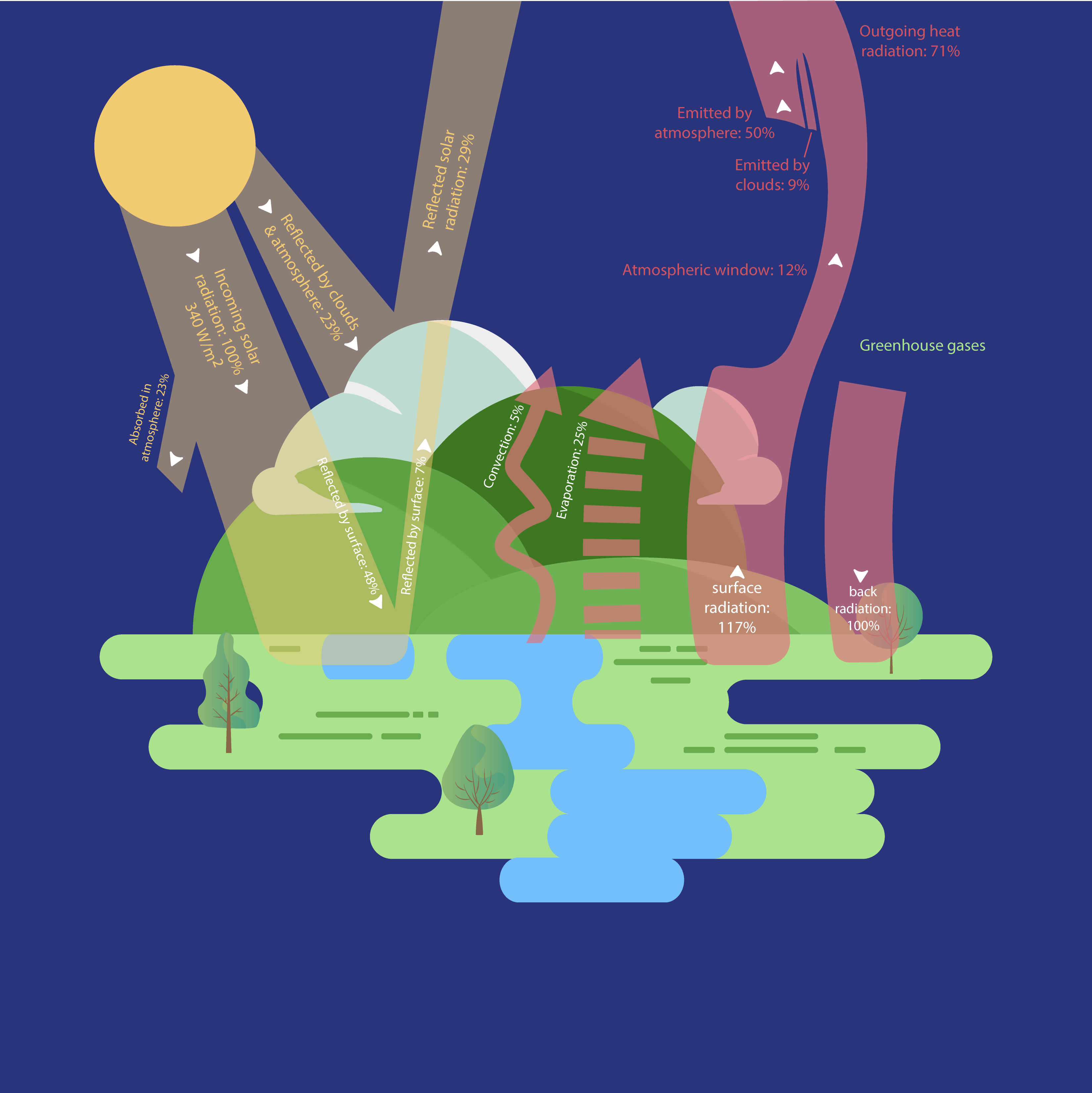
In addition to emitting infrared radiation, Earth’s surface transfers energy to the atmosphere via two other pathways: evaporation and convection (Fig. 4.1). About 25% of absorbed solar radiation drives the evaporation of liquid water into water vapor. The latent energy in the water vapor gets transferred to the atmosphere as it cools. About 5% of the surface absorbed solar radiation powers convective air currents, which also move energy from the surface to higher elevations in the atmosphere. There is a small discrepancy in the surface energy budget. The proportion of solar energy flowing from the surface to the atmosphere via infrared radiation (17%), evaporation (25%), and convection (5%) only adds up to 47%, not the total 48% of incoming solar radiation that is absorbed by the surface. The missing 1% is captured by photosynthetic organisms that store the energy in the chemical bonds of carbohydrates. Eventually, most of that captured energy will get released again relatively quickly as heat when organisms use it to power their activities or when it is released during the combustion of biomass. But a fraction of it does get put into relatively long-term storage in the soil or as fossilized biomass. Figure 4.1 doesn’t account for photosynthesis because it is such a small line item in Earth’s daily energy budget. But our use of the long-term energy stored in fossil fuels as well as our disruption of the biologically mediated energy flows are profoundly influencing Earth’s energy budget indirectly through their influence on the carbon system.
4.2 Drivers, Forcings, Feedbacks, and Tipping Points
Section 4.2: Drivers, Forcings, Feedbacks, and Tipping Points
Earth’s temperature as well as nearly all the other aspects of its climate are governed by the dynamic balance between energy inputs and energy outputs. That balance is in turn influenced by a wide range of factors that alter the amount and rate of energy flowing through various parts of the system. These factors are called climate drivers. For example, relatively dark-colored surfaces such as vegetation and water absorb more shortwave solar radiation than relatively light-colored surfaces such as clouds and ice. As a result, the relative proportions of those elements are important climate drivers. Similarly, atmospheric gasses differ in their relative ability to absorb shortwave and longwave radiation. Perhaps the most famous climate driver is the abundance of CO2 in the atmosphere, which is relatively good at absorbing longwave radiation.
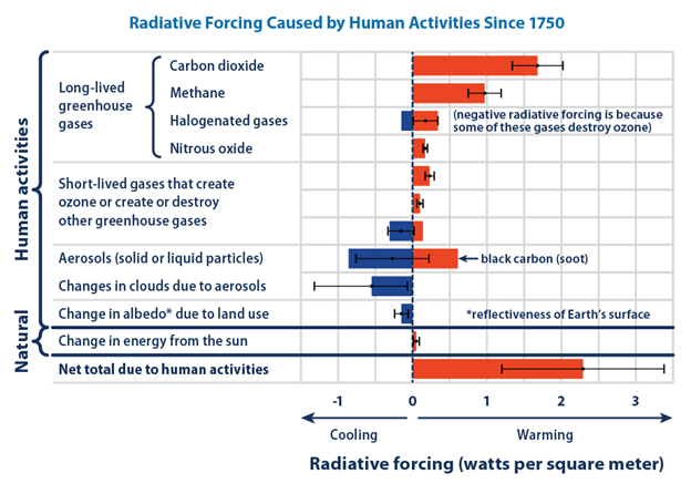
The influence that climate drivers have on Earth’s energy balance varies over time as factors such as their abundance change. The slowly increasing energy output form the sun is one example. Another example is the increasing abundance of greenhouse gasses in the atmosphere. Radiative forcing is a metric that describes the degree to which change in a climate driver over time has caused a change in Earth’s net energy balance. Forcing is measured as an energy flux (W m-2) relative to some benchmark, such as what the energy balance was at some point in the past. A commonly used benchmark year is 1750, which is Earth’s energy state just before widespread industrialization. Climate forcing can be positive (contributing to warming) or negative (contributing to cooling). Figure 4.2 summarizes the radiative forcing caused by our activities since 1750. Over that time, our cumulative activities have increased Earth’s energy balance by about 2.3 W m-2.10 We are by far the strongest current perturbation to Earth’s energy balance. Natural drivers such as changes in solar output and volcanic eruptions have had a comparatively tiny impact on the energy balance. For instance, since 1750, the slowly increasing solar output has caused a positive radiative forcing of only about 0.12 W m-2, while aerosols from volcanic eruptions have had a negative forcing of about -0.06 W m-2.11
Our biggest effect on Earth’s energy balance has been through generating greenhouse gases, mainly the carbon-containing molecules of carbon dioxide (CO2) and methane (CH4), and the magnitude of greenhouse gas forcing has been increasing since the start of the agro-industrial era. In 2019, greenhouse gas forcing was 45% more than what it was in 1990.12 The radiative forcing associated with the greenhouse gasses in Figure 4.2 reflects both their abundance in the atmosphere as well as their relative ability to absorb radiative energy. Greenhouse gasses differ in their energy-absorbing properties. They also have different lengths of time that they persist in the atmosphere before chemical reactions convert them to something else. As a result, greenhouse gases differ in their innate influence on Earth’s energy balance.
A metric used to describe that differential impact is called global warming potential (GWP). GWP is a measure of how much energy 1 ton of a gas will absorb over a given period (i.e., its radiative forcing) relative to the emissions of 1 ton of carbon dioxide. One hundred years is the typical period used for comparison, but other time frames are sometimes used. By definition, CO2 has a GWP of 1. CO2 was chosen as the benchmark because it is the greenhouse gas we emit the most and because it can persist in the atmosphere for thousands of years. CH4 absorbs much more energy than CO2, but it lasts only about a decade or so in the atmosphere; the net result is a GWP of 28–36 times that of CO2 over 100 years. Nitrous oxide (N2O) has a GWP 265–298 times that of CO2 over 100 years.13 We can use GWP as an accounting tool to simplify adding up the cumulative impact of our greenhouse gas emissions. One standardized metric is CO2 equivalent (CO2e). CO2 equivalent is calculated by multiplying the amount of a greenhouse gas by its global warming potential. For example, 100 kg of N2O has the same global warming potential over 100 years as 29,800 Kg of CO2 (100 × 298) using the high-end GWP estimate. CO2 equivalents are particularly handy to use for describing the cumulative impact of activities that generate multiple greenhouse gasses. Figure 4.2 gives a simple example.
| A Small Farm's Aggregate Greenhouse Gas Emissions: A Sample Calculation | |||
|---|---|---|---|
| Emission type | Annual amount (kg) | Global warming potential | CO2 equivalent (kg CO2e) |
| CO2 from farm machinery | 725 | 1 | 725 |
| CH4 from dairy cows | 500 | 36 | 18,0000 |
| N2O from fertilizer use | 2.5 | 298 | 745 |
| Total Emissions: | |||
| 19,470 | |||
Climate drivers also interact with each other, creating climate feedbacks that either amplify (positive feedbacks) or dampen (negative feedbacks) the net effect on climate. A classic positive feedback involves Earth’s ice cover.
Ice cover has a strong influence on climate because it reflects away a lot of incoming solar radiation before it can get absorbed by the Earth System. In physics jargon, it has a high albedo. The amount of ice cover itself is influenced by climate. Any increase to global temperature caused by other factors—such as greenhouse gas emissions—can cause a loss of ice cover that in turn leads to further increases in temperature and yet more loss of ice cover. The feedback can also go in the opposite direction, with cooling temperatures creating more ice that cools temperature even more.
The ice-albedo feedback, as it is called, helped create the fluctuating cycles of warm and cold periods that characterized Earth’s climate during the Pleistocene.14 Other positive climate feedbacks involve greenhouse gasses. For example, the permafrost of Earth’s arctic regions currently stores about 1,400 Gt of carbon in the form of frozen plant biomass. That’s almost twice the amount that is currently in the atmosphere National Snow and Ice Data.15 Warmer conditions can thaw the permafrost, causing decomposition and the release of greenhouse gasses, namely methane (CH4) and carbon dioxide (CO2). Those in turn create warmer conditions that thaw more permafrost. We can observe this feedback happening. Autumn carbon dioxide emissions from the tundra near Utqiaġvik, Alaska, have increased by 73% since 1975, primarily from warming soils. The Alaska tundra is now a net exporter of CO2, and in 2013-2014, this more than offset net carbon fixed by other Alaska ecosystems such as boreal forests and made all terrestrial Alaska a net source of CO2 to the atmosphere.16
There are also a range of negative feedbacks that tend to dampen the effects of climate drivers. For example, plants that have access to higher concentrations of atmospheric CO2 carry out more photosynthesis, a phenomenon known as the CO2 fertilization effect. Photosynthesis also speeds up with increasing temperature. These relationships create a stabilizing negative feedback: as atmospheric CO2 increases and global temperature rises, more CO2 gets pulled out of the atmosphere by photosynthesis, thus reducing atmospheric CO2 and decreasing temperature. The CO2 that we have been adding to the atmosphere has caused a plant growth spurt (particularly in the tropics) that currently sops up as much as 30% of our annual CO2 emissions.17
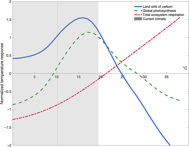
The interactions among climate drivers as well as the biophysical processes that underlie the drivers are often complex and don’t have simple linear relationships. The storage of carbon in plant biomass is a good example. The 30% of our annual CO2 emissions that vegetation currently absorbs is the net difference between gross ecosystem primary productivity (carbon uptake by vegetation) and total ecosystem respiration (carbon loss to the atmosphere). That value is called net ecosystem productivity (NEP), and it is a measure of the strength of the flow of atmospheric CO2 into terrestrial storage. NEP increases with temperature, but the pattern is not linear because photosynthesis and respiration have different temperature patterns. The rate of photosynthesis increases with temperature until it reaches an optimal peak, then it rapidly declines with further temperature increases. The temperature optimum for photosynthesis varies a bit across species and ecosystems, but it tends to be between 18°C and 24°C. In contrast, respiration continues to rapidly increase with temperate even past 38°C. The net result is that NEP has a temperature optimum as well as a higher-end temperature threshold beyond which NEP turns negative as respiration exceeds photosynthesis.
Normalized across all terrestrial ecosystems, the temperature optimum for NEP is about 16°C, and the maximum threshold is 25°C (Fig. 4.3). We have already warmed the planet to the point that the aggregate terrestrial biosphere is slightly past its NEP optimum. NEP will continue to decrease as global temperature increases, until it stops altogether at the 25°C. That threshold is a powerful climate tipping point, beyond which the climate system is radically altered into one where the terrestrial biosphere is a net exporter of CO2 instead of a net sink for it. Currently, less than 10% of the terrestrial biosphere experiences temperatures that are higher than the optimum for NEP, but that could increase to 50% by the end of the century if we continue emitting greenhouse gasses at our currently high rate. Earth’s most productive ecosystems, such as tropical rainforests and boreal forests, are already close to their NEP tipping points, so that we could lose as much as 45% of the terrestrial carbon sink by midcentury.18
There are other potential climate tipping points that could push the Earth System into abrupt or largely irreversible changes. For instance, we have evidence that both the Greenland and West Antarctic ice sheets are prone to sudden loss of volume and collapse, similar to how a seemingly stable sandcastle can suddenly fall into the sea. That would result in a dramatically more rapid rise in sea level than if the ice sheets melted more slowly and steadily, like a block of ice on a solid table.19
Disentangling the net effect on climate of all the changing drivers, their feedbacks, and potential tipping points gets to be complex, but it is an important task if we want to understand how our perturbations to the Earth System are likely to alter climate in the future. Some climate models suggest that under some circumstances, feedbacks among climate drivers can cause abrupt and catastrophic swings. We have some evidence that the climate system has indeed experienced some scarily close meltdowns in the past. About 252 mya, at the end of the Permian, average global temperature spiked by as much as 6°C, creating a crazy hot world. Some estimates suggest that equatorial sea surface temperatures may have reached an amazing 40°C, the temperature of a hot tub and lethal for most marine organisms.20 As much as 95% of the species on the planet were wiped out. One hypothesis for what happened is that a positive feedback developed that caused a runaway greenhouse effect. The initial trigger was a massive and prolonged volcanic eruption—whose flows today cover a 2 million km2 region called the Siberian Traps. The eruption injected a large slug of greenhouse gasses into the atmosphere that warmed the planet enough to start melting vast stores of frozen methane hydrate in ocean sediments. The resulting atmospheric spike of this powerful greenhouse gas caused further warming that melted more methane hydrate, causing more warming.21 Eventually, negative feedbacks acting over slower timescales, such as the weathering of silicate rocks, stabilized the climate. Understanding how feedbacks such as these dynamically alter (or stabilize) climate over time is one of the biggest challenges of climate science.
4.3 The Carbon System (in Ten Chemical Equations)
Section 4.3: The Carbon System (in Ten Chemical Equations)
Humans generate the main carbon-containing greenhouse gasses through a range of activities that convert carbon stored in the biomass of organisms and in various mineral forms (principally fossil fuels). In doing so, we have transformed the global flow of carbon.
At any given moment, Earth’s carbon is sitting in or flowing between five main reservoirs: the atmosphere, the bodies of living organisms and their dead parts, soil and sediment, the rocky crust, and the ocean (Fig. 4.4; see also 3.10). Within each of these main reservoirs, carbon exists in a range of forms or sub-reservoirs that vary in characteristics such as their longevity. In the atmosphere, carbon exists mainly as part of carbon dioxide (CO2) and methane (CH4) gas molecules. In organisms, carbon is present in a diverse range of carbohydrates that include ephemeral forms such as glucose molecules as well as more robust and long-lived structures like the wood of giant sequoias. In addition, some organisms such as corals and foraminifera fix carbon as calcium carbonate (CaCO3) to form shells and exoskeletons. As coral atolls illustrate (see Chap. 3), CaCO3 structures can last millions of years.
In soil and sediment, carbon exists as the products of photosynthesis in various stages of decay as well as the byproducts of organism metabolism. Under some conditions (e.g., waterlogged, frozen, dry), decomposition grinds to a halt, and the carbon can sit around for a long time. A good example of carbon cold storage is the methane hydrate whose melting contributed to the positive feedback that may have driven the end Permian temperature spike described above. In the crust, carbon is stored in less dynamic carbonate minerals such as limestone as well as hydrocarbons (the mineralized remains of organic matter). Although these minerals tend to store carbon for a long time, they aren’t static storage. Rock weathering (equations (4.5) and (4.6)), volcanism, and calcium carbonate formation (equation (4.3)) move carbon into and out of the crust. In the oceans, most of the carbon is in the form of dissolved inorganic carbon (DIC), which consists of dissolved CO2, carbonic acid (H2CO3), bicarbonate (HCO3−), and carbonate (CO32−). The rest is dissolved as fine bits of organic matter (dissolved organic carbon (DOC)).
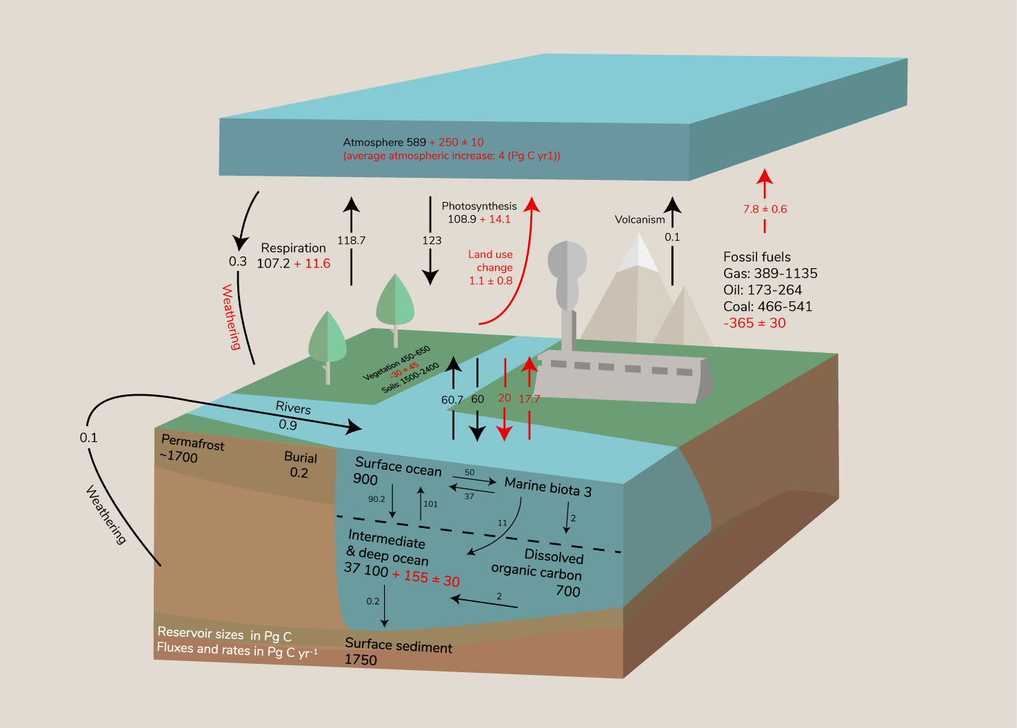
By far the biggest reservoir of carbon is Earth’s crust. Sedimentary rocks contain about 100,000,000 petagrams of carbon (Pg C), and hydrocarbons contain about another 2,000 Pg C. The oceans are the second biggest reservoir, storing about 37,800 Pg C in its various dissolved forms, followed by soil and sediment (5,850 Pg C), the atmosphere (829 Pg C), and the bodies of organisms (653 Pg C). These reservoir sizes are not static. A range of processes shuttle carbon between each of the different reservoirs (Fig. 4.4). This flow is often described as a cycle, since a carbon atom could conceivably make its way through all the different reservoirs in an endless loop. But another way to think about the flow is as a system that maintains a dynamic equilibrium of carbon among the different reservoirs, similar to the energy budget in Figure 4.1. One important difference from the energy budget is that the carbon system is closed (except for the small fraction of carbon that is swept into space by the solar wind or that is deposited by comets and asteroids). If carbon leaves one reservoir, it has to flow into another reservoir somewhere else. The processes that move carbon between reservoirs operate at different rates and over different timescales. They also tend to interact with each other, forming some of the complex feedback loops mentioned in the previous section. From an ecosystem standpoint, there are three main types of flow pathways: biologically mediated ones, abiotic ones, and human ones.
Biologically Mediated Pathways
There are three main biologically mediated pathways. Not surprisingly, they tend to be fast and play out over biologically meaningful timescales such as years and decades. Perhaps the most obvious one is photosynthesis. Photosynthetic organisms move CO2 out of the atmosphere and the ocean’s dissolved inorganic reservoir and fix it in carbohydrate molecules.
[latex]6CO_2 + 6H_2O \rightarrow C_6H_{12}O_6 + 6O_2\tag{4.1}[/latex]
[latex]\small{\text{carbon dioxide + water = glucose + oxygen}}[/latex]
The process is quick; plants can synthesize a molecule of glucose in as little as 30 seconds. The complementary process is respiration, which just as quickly moves carbon stored in carbohydrates back to the atmosphere or the dissolved inorganic ocean pool.
[latex]C_6H_{12}O_6 + 6O_2 \rightarrow 6CO_2 + 6H_2O\tag{4.2}[/latex]
[latex]\small{\text{glucose + oxygen = carbon dioxide + water}}[/latex]
The two pathways are almost (but not quite) balanced. A small fraction of the carbon fixed in photosynthesis escapes the clutches of respiring organisms and settles into deep ocean sediments or gets locked in anoxic or frozen soils. Some of the carbon in ocean sediment eventually gets transformed into sedimentary rocks or into hydrocarbons, where it can stay for a long time until it reemerges millions of years later as uplifted sedimentary rock, as CO2 released in a volcanic eruption, or out the end of an oil and gas well.
The third main biologically mediated pathway for carbon is the formation of calcium carbonate (CaCO3) shells by some phytoplankton species (coccolithophores and foraminifera), corals, and a few larger organisms like clams. The process moves bicarbonate out of the ocean reservoir of dissolved inorganic carbon and fixes it in hard shells.
[latex]Ca^2+ + 2HCO^{−3} \rightarrow CaCO_3 + CO_2 + H_2O\tag{4.3}[/latex]
[latex]\small{\text{calcium ions + bicarbonate ions = calcium carbonate + carbon dioxide + water}}[/latex]
Over the short term, the formation of CaCO3 increases the amount of dissolved CO2 in the ocean, which (along with lowered ocean pH) drives some dissolved CO2 into the atmosphere. That flow of carbon is often referred to as the calcium carbonate counter-pump because it acts against marine photosynthesis that is sucking CO2 out of the atmosphere. Over longer timescales, however, some calcium carbonate shells sink into deep ocean sediments where they get transformed into sedimentary rocks such as limestone. This flow coupled with the weathering of silicate rocks (equation (4.6)) is one of the major pathways by which carbon moves from the atmosphere to the crust, and over long geologic timescales, it has had a significant moderating influence on Earth’s energy balance.22
Abiotic Pathways
There are also three main abiotic pathways through which carbon flows. These tend to operate at slower rates and over longer time frames than the biologically mediated pathways, but two of them are tightly linked to the biological pathways. The first of these is the flow of CO2 into and out of the surface water of the oceans. CO2 moves between the ocean and atmosphere through diffusion, just like in a fizzy drink. Dissolved CO2 then forms carbonic acid (H2CO3) that itself dissociates into bicarbonate (HCO3−) and hydrogen ions (H+). The bicarbonate also further disassociates into carbonate ions (CO32−) and more hydrogen ions:
[latex]CO_2 + H_2O \rightleftharpoons H_2CO_3 \rightleftharpoons H^+ + HCO_3^− \rightleftharpoons 2H^+ + CO_3^{2−}\tag{4.4}[/latex]
[latex]\small{\text{carbon dioxide + water = carbonic acid}}[/latex]
[latex]\small{\text{= hydrogen ions + bicarbonate ions = hydrogen ions + carbonate ions}}[/latex]
Collectively, these forms of carbon make up the dissolved inorganic pool. The double arrows in equation (4.4) indicate that the reactions can readily flow in either direction. The flow of carbon back and forth between the ocean and atmosphere is one of the largest annual fluxes in the carbon system. The rate and magnitude of the flow in each direction are governed by four main factors: (1) the strength of the diffusion gradient in CO2 determined by the relative amounts of CO2 in the atmosphere and surface ocean; (2) the rate of photosynthesis and calcium carbonate formation, which alter the concentration of dissolved CO2 and thus the diffusion gradient; (3) the degree of mixing between surface and deeper ocean water, which also alters the diffusion gradient; and (4) the temperature and salinity of the ocean, which change the solubility of CO2 in seawater. The exchange of CO2 between surface water and the atmosphere happens relatively quickly, but the movement of carbon to deeper ocean depths and into marine sediments goes much slower, on the order of thousands of years.
Carbonic acid also forms when CO2 dissolves in rainwater, and this starts the second main abiotic carbon pathway: rock weathering. Acting slowly but relentlessly over millions of years, slightly acidic rainwater dissolves carbonate rocks (e.g., limestone, dolomite) into calcium bicarbonate:
[latex]H_2CO_3 + CaCO_3 = Ca\left(HCO_3\right)_2 \tag{4.5}[/latex]
[latex]\small{\text{carbonic acid + calcium carbonate = calcium bicarbonate (in solution)}}[/latex]
It also dissolves silicate rocks (e.g., feldspar, olivine) into calcium, bicarbonate ions, and silicic acid. There are a wide variety of silicate minerals; equation (4.6) uses calcium silicate (CaSiO3) as an example:
[latex]2CO_2 + 3H_2O + CaSiO_3 = Ca^{2+}+ 2HCO_3^– + H_4SiO_4 \tag{4.6}[/latex]
[latex]\small{\text{carbon dioxide + water + calcium silicate}}[/latex]
[latex]\small{\text{= calcium ions + bicarbonate ions + silicic acid (in solution)}}[/latex]
The calcium and bicarbonate freed by rock weathering flow through streams and rivers to the ocean, where shell-forming organisms use them to form calcium carbonate (equation (4.3)). Some of that will eventually be transferred back into long-term storage as carbonate minerals. Notice that silicate rock weathering uses two units of atmospheric CO2 (the left side of equation (4.6)), while calcium carbonate shell formation produces only one unit of CO2 as a by-product (the right side of equation (4.3)). This means that the combination of silicate rock weathering and calcium carbonate shell formation eventually results in a net transfer of CO2 from the atmosphere into long-term storage as carbonate rock. As mentioned above, this process is a significant climate driver over long timescales. It often acts as a stabilizing negative feedback on climate. For example, volcanic eruptions put CO2 into the atmosphere, but they also move deep minerals to the surface and create steep, uplifted terrain. Those in turn increase rock weathering, which over a longer time frame counteracts the volcanic CO2 emissions.
The release of CO2 in volcanic eruptions is the third major abiotic carbon flow. This is a major pathway by which carbon locked in sedimentary rocks reenters the atmosphere. In contrast to weathering, volcanic eruptions can release a lot of CO2 over a very short time. Extensive and prolonged eruptions in the past, such as those that formed the Siberian Traps 250 mya, have at times dramatically increased atmospheric carbon. But most eruptions tend be sporadic and limited in scale so that on average they contribute a tiny amount to increasing atmospheric carbon.
Human-Driven Flows
We have added three new significant flows to the carbon system. First, we are burning fossil fuels, which moves carbon stored as hydrocarbons into the atmosphere primarily as CO2.
[latex]C_xH_y + n(O_2) \rightarrow x(CO_2) + y/2 (H_2O) \tag{4.7}[/latex]
[latex]\small{\text{hydrocarbons + oxygen = carbon dioxide + water}}[/latex]
Equation (4.7) is a general one that works for all the different hydrocarbons we burn. The x’s are the number of carbons in the hydrocarbon molecule or the number of CO2 molecules that result from combustion; the y’s are the number of hydrogens in the hydrocarbon or the number of water molecules that result; n is the number of O2 molecules. Note the similarity to equation (4.2). In fact, I could have used equation (4.7) to describe biological respiration instead of equation (4.2). When we burn fossil fuels, we are essentially respiring the carbon fixed by the photosynthesis of past ecosystems.
We do something similar in our second pathway: the production of concrete. When we make concrete, we release carbon stored as calcium carbonate formed by past ecosystems (equation (4.3)). The production of Portland cement (a main ingredient of concrete) starts by making quicklime (calcium oxide) from calcium carbonate.
[latex]CaCO_3 + \text{heat} \rightarrow CaO + CO_2 \tag{4.8}[/latex]
[latex]\small{\text{calcium carbonate + heat = calcium oxide + carbon dioxide}}[/latex]
In 2019, this innocuous process surprisingly accounted for 4% of our yearly CO2 emissions.23. But concrete also acts as a sink for carbon after it is formed. Over time, CO2 and water diffuse through pores in the cement, where they start a series of chemical reactions known as carbonation. The net result is the re-formation of calcium carbonate. Carbonation is a concern for structural engineers because over time, it can weaken the structural integrity of concrete structures. But carbonation has also offset 43% of the direct CO2 emissions from the production of cement.24
Our third pathway involves land use changes that directly and indirectly alter carbon flows in several ways (see also Chap. 3). By creating domesticated urban and agricultural landscapes, we now appropriate about 25% of Earth’s potential net primary production (NPP).25 This appropriated NPP reflects atmospheric carbon that has been stored or would otherwise have been stored as biomass. We funnel this appropriated NPP into pathways that tend to foster its relatively quick conversion into greenhouse gasses. We eat the biomass, feed it to livestock, turn it into clothes, or use it as biofuel, all of which release a significant portion of the stored carbon via respiration (equation (4.3)). We also often use fire to clear vegetation, which even more quickly moves carbon to the atmosphere via combustion (equation (4.7)). In many places, clearing forests and draining wetlands create conditions that favor the biological respiration of aerobic soil decomposers (equation (4.3)). In other situations, we create conditions that favor methane-producing microorganisms (methanogens). Some forms of rice production involve periodically flooding fields. The waterlogged and anaerobic conditions favor methanogens that decompose organic matter in the soil. Soil methanogens produce methane through several biochemical pathways, but a main one uses acetate:
[latex]CH_3COO^– + H^+ \rightarrow CH_4 + CO_2 \tag{4.9}[/latex]
[latex]\small{\text{acetate ions + hydrogen ions = methane + carbon dioxide}}[/latex]
We also feed a significant chunk of the appropriated NPP to ruminant livestock such as cows. The guts of ruminants are habitat for methanogens that use a different metabolic pathway than that of soil microorganisms:
[latex]CO_2 + 4 H_2 \rightarrow CH_4 + 2 H_2O \tag{4.10}[/latex]
[latex]\small{\text{carbon dioxide + hydrogen = methane + water}}[/latex]
Methane constitutes about 16% of our total greenhouse emissions and 41% of that is generated by ruminant livestock and rice cultivation.2627
Shock to the System
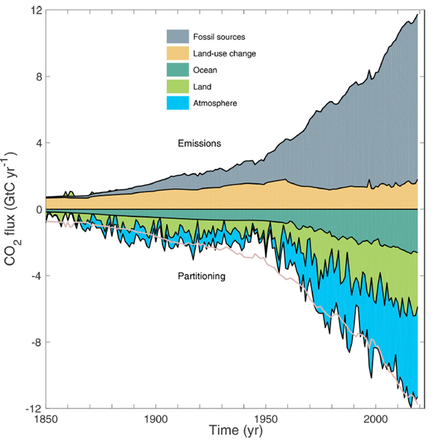
Our land use changes and burning of fossil fuels have been moving carbon from soil, crust, and biomass into the atmosphere. From 2010 to 2019, that human-caused flow averaged 11 Pg C per year.28 The added carbon is a large perturbation that ripples through the entire carbon system. Increased atmospheric CO2 spurs the CO2 fertilization effect that has been pulling 3.4 Pg C per year back out of the atmosphere in the form of biomass. Greater atmospheric CO2 also increases CO2 diffusion into the ocean, causing net ocean uptake of another 2.5 Pg C per year. Still, those powerful feedbacks only account for 5.9 Pg C, which means that the size of the atmospheric reservoir grew by a net average of 5.1 Pg C per year from 2010 to 2019.29
That growth rate has itself been accelerating. In the 1960s, atmospheric CO2 was increasing at an average rate of 1.8 Pg C per year. By the 1990s, it had increased to 3.2 Pg C per year. During the first decade of the twenty-first century, it was 4 Pg C per year. Note that Figure 4.4 uses the 2000-2009 averages, so the values it reports are already out of date. At the start of agro-industrialization, most of our carbon emissions were the result of land use changes associated with clearing land for agriculture and cities, and most of the resulting emissions either flowed back into photosynthesis or were absorbed by the oceans. But the burning of fossil fuels became our dominant source of carbon emissions, and the atmosphere increasingly has become the medium-term destination for the carbon (Fig. 4.5).
Calling these changes a perturbation implies a little nudge. A violent body slam is probably a more apt description. There probably hasn’t been this much CO2 in the atmosphere since the middle of the Pliocene 3-5 mya,30 and the current pace of change in atmospheric carbon is the fastest it has been for at least the past 800,000 years (see 1.11). We have to look to some of the great cataclysmic periods in Earth’s more distant past to find comparably fast changes to the carbon system. One potential analog is the spike in atmospheric CO2 that triggered the end Permian mass extinction described above. One study estimates the rate of CO2 emissions during that period at 0.7 Pg C per year, more than 14 times less than our current emission rate.31 The comparison is not perfect. The end Permian emissions continued for thousands of years, something we won’t be able to replicate even if we managed to burn all the available fossil fuel reserves. Still, although we have only been at it for a few hundred years, our carbon shock is already profoundly altering Earth’s climate.
4.4 Supercharged Climate
Section 4.4: Supercharged Climate
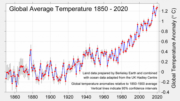
The 2.3 W m-2 that we have so far increased Earth’s energy budget by has raised its temperature (Fig. 4.6). Much of the increased warmth has occurred over just the past 50 years. The 10 warmest years in the historical record have occurred since 2005. In 2020, the El Niño-Southern Oscillation (ENSO) was in a cool La Niña phase that typically reduces average global temperature. Despite that, 2020 was still the second-warmest year on record, 1.2°C warmer than the average during the last half of the nineteenth century (1850-1900) World Meteorological.32 Just as the rate of CO2 accumulation in the atmosphere has been accelerating, so has global temperature. Since 1880, Earth’s temperature has been rising an average of 0.08°C per decade, but the rate since 1981 has been more than twice that at 0.18°C per decade.33
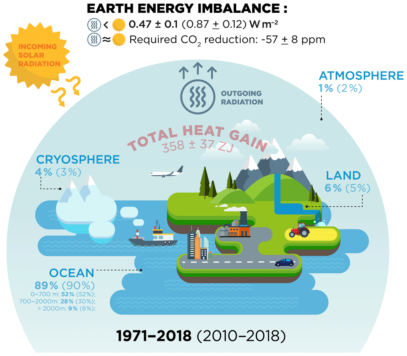
A 1° increase in average surface temperature since the nineteenth century may sound like a trifling thing, but it represents a huge shift in our climate. Keep in mind that averaging temperature over the entire year and across all the different ocean and land surfaces of the planet mutes the daily and site-specific extremes that we experience as individuals. Just as importantly, a lot of the retained heat energy has been absorbed into parts of the Earth System that are not directly reflected in the global surface temperature. Overall, Earth accumulated 3.58 and 1023 J of energy between 1971 and 2018, 89% of which was absorbed by the ocean (Fig. 4.7). About one-third of that total retained heat has warmed deep ocean waters below 700 m, which doesn’t directly contribute to surface temperature. Similarly, smaller fractions have been sucked up by melting ice as well as the convection and evaporation energy pathways in the atmosphere.
All that accumulating heat energy is supercharging the Earth System and altering almost every aspect of its climate. Understanding how 3.58 and 1023 J (and counting) of added energy translates into all the different aspects of climate such as rainfall patterns or when the first winter frosts happen is an amazingly complex and difficult task. Also, from the perspective of individual organisms, the local and short-term manifestations of climate are more important than broad global metrics such as the decadal average surface temperature. Despite the challenges, we are beginning to develop a detailed picture of how Earth’s climate is changing. There are five broad aspects to the changes.
Changing Ocean and Atmosphere Circulation Patterns
The simplified energy budget in Figure 4.1 doesn’t account for the variability in where and when energy enters and leaves the Earth System. Earth’s spherical shape, its axial tilt, and its slightly wobbly rotation create marked spatial and temporal variation in incident solar radiation. In addition, landscapes vary in how much solar radiation they absorb. For instance, bright ice absorbs a lot less than dark ocean. At a big scale, these differences create a net heating imbalance between polar regions and the tropics that drives the global circulation of atmosphere and ocean currents.34 Those flows of energy, air, and water help generate the characteristic attributes of more regional and local climate that in turn strongly influence ecosystem characteristics and functions (see Chap. 3).
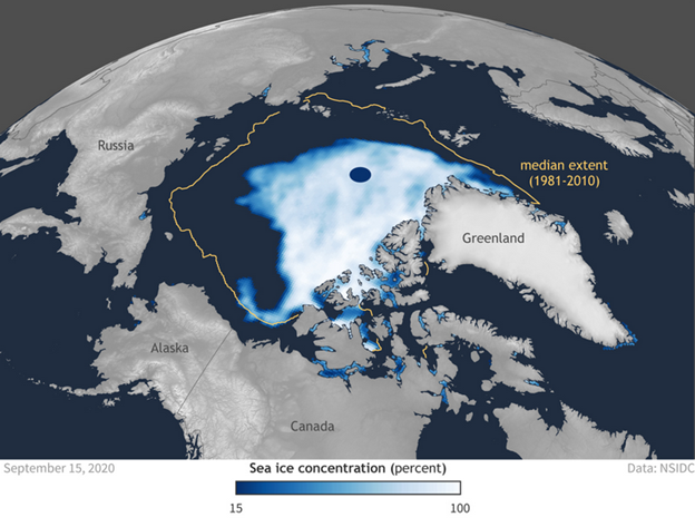
These spatial flow patterns are changing as the Earth retains more heat energy. One big-picture change is that polar regions have been warming faster than tropical ones, and as a result the temperature differential between the poles and tropics is becoming less pronounced. The Arctic has been warming particularly fast. From 1971 to 2019, the Arctic warmed by 3.1°C, three times faster than the global average.35 The Arctic’s rapid warming is being driven by several interacting factors known collectively as arctic amplification. One important factor is the ice-albedo feedback that I describe above, which affects not only the global temperature balance but also local arctic temperatures. Since 1978 the extent of arctic sea ice at the end of summer has been declining by an average of 13.1% per decade relative to the 1981–2010 average.36 The 2020 end-of-summer arctic sea ice extent was the second lowest so far recorded (Fig. 4.8).
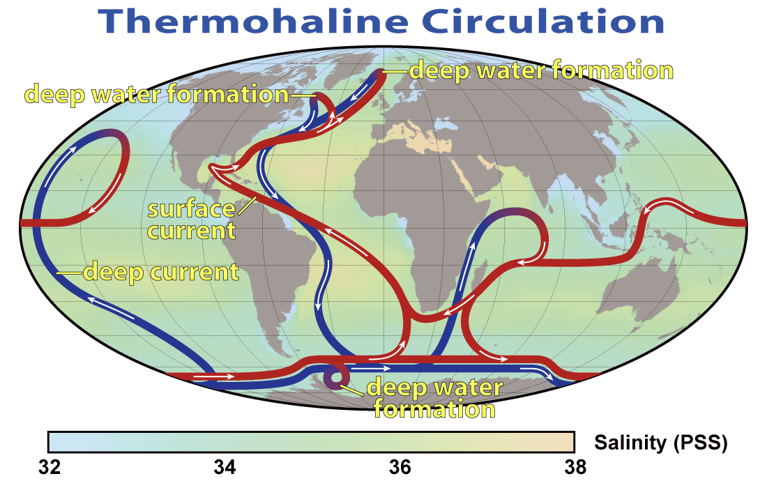
The narrowing temperature imbalance between the tropics and poles is altering ocean and air currents, although our understanding of these changes is still not complete. One example is what is happening to Earth’s epic circulation of water known as the thermohaline circulation system (Fig. 4.9). As warm equatorial water flows toward the poles, it loses its heat and gets denser. In a few places, most notably off the southern coast of Greenland, the water also gets saltier as the result of sea ice formation, which locks up some water leaving the salt behind. The combination of cold and salty makes the surface water dense enough to sink and flow horizontally as deep ocean currents. The constant push of surface water down eventually forces water back up in the equatorial Pacific and Indian Oceans. It takes about 1,000 years for water to complete a circuit, but the grand circulation has components with far more immediate influence on regional climate. For example, a critical leg of the global thermohaline circulation is the Gulf Stream, which rapidly moves warm equatorial water into the North Atlantic where it releases heat, gets salty, and sinks. That transfer of heat significantly influences the climate of the entire Northern Hemisphere.37 Disconcertingly, the Gulf Stream is currently moving more slowly than it has in at least 1,600 years.38 What seems to be happening is that fresh water pouring off of Greenland’s melting ice cap is making surface water in the North Atlantic less salty and dense, inhibiting it from sinking.
The slowdown in heat transfer is already having an effect on regional climate. With less heat coming from the Gulf Stream, the North Atlantic is one of the few places on Earth that has been getting colder over the past 50 years.39 At the same time, the course of the now more sluggish Gulf Stream has meandered west, causing warm water to back up along the eastern coast of the United States and Canada. That is exacerbating the threat of sea level rise for coastal communities in the region and causing the Grand Banks, one of the world’s great fisheries, to be among the fastest warming parts of the ocean.4041 The North Atlantic cool patch may also be contributing to an increased intensity of European heat waves by influencing the flow of the polar jet stream.42 These early changes to regional climate may just be the beginning. There is evidence that past disruptions to the thermohaline circulation acted as a climate tripping point, contributing to the abrupt swings between glacial and interglacial periods that occurred during the climactically tumultuous Pleistocene.43
The rapid warming of the Arctic may also be causing changes to global air circulation patterns. Similar to what happens in the ocean, Earth’s air makes a big three-dimensional circuit: warm air rises at lower latitudes, travels poleward until it cools, and sinks at higher latitudes. That general flow gets nudged by the forces of Earth’s rotation and deflected by Earth’s surface geography into wavelike patterns called planetary waves (also called Rossby waves). Like radio waves that transmit all the content we consume on mobile phones, planetary waves transmit much of the weather we experience. The waves generally move slowly from west to east, but they interact with the much faster-flowing winds that make up the jet streams.44
Their interaction causes the jet streams to have giant meanders from their generally east to west flow. Those meanders let warm low-latitude air into polar regions and cold polar air into low latitudes. The resulting mix of the different air masses helps to generate weather phenomena like warm and cold fronts. Because the underlying planetary waves move slowly, the jet stream meanders can keep their shape and position for a long time, creating persistent local weather patterns. The weeks of endless rainstorms that the US Pacific Northwest often experiences are the result of a persistent jet stream meander that directs the path of low-pressure systems into the region.
There is evidence that the weakening temperature differential between the poles and midlatitudes is causing the jet stream meanders to be more pronounced and to hold their position for longer periods.45 This could be playing a role in helping to produce more extreme weather events (see Figure 4.10 below). For example, the position of the polar jet stream where it flows over the North Atlantic strongly influences weather in Europe by directing where storms go and where high-pressure systems sit. In one study, researchers used tree ring data to help reconstruct the position of the North Atlantic jet stream all the way back to the year 1725. The researchers found that big swings northward in the jet were associated with heat waves and droughts in northwestern Europe, while big southward swings were associated with wildfires in southeastern Europe. The researchers also found that the jet stream has been getting wavier since the 1960s, with an increasing frequency of abnormally large swings north and south.46 That study did not identify a reason for why the jet stream has been getting wavier, and in general the connection between climate change and jet stream conditions is currently not clear. There is a lot of conflicting evidence that doesn’t support a link between warming conditions in the Arctic and altered atmosphere flow patterns in lower latitudes.47 Our uncertainty partly reflects the difficulty in linking broad long-term changes in climate to the shorter-term flow patterns that affect weather.48
Changes to Local Average Temperature and Precipitation
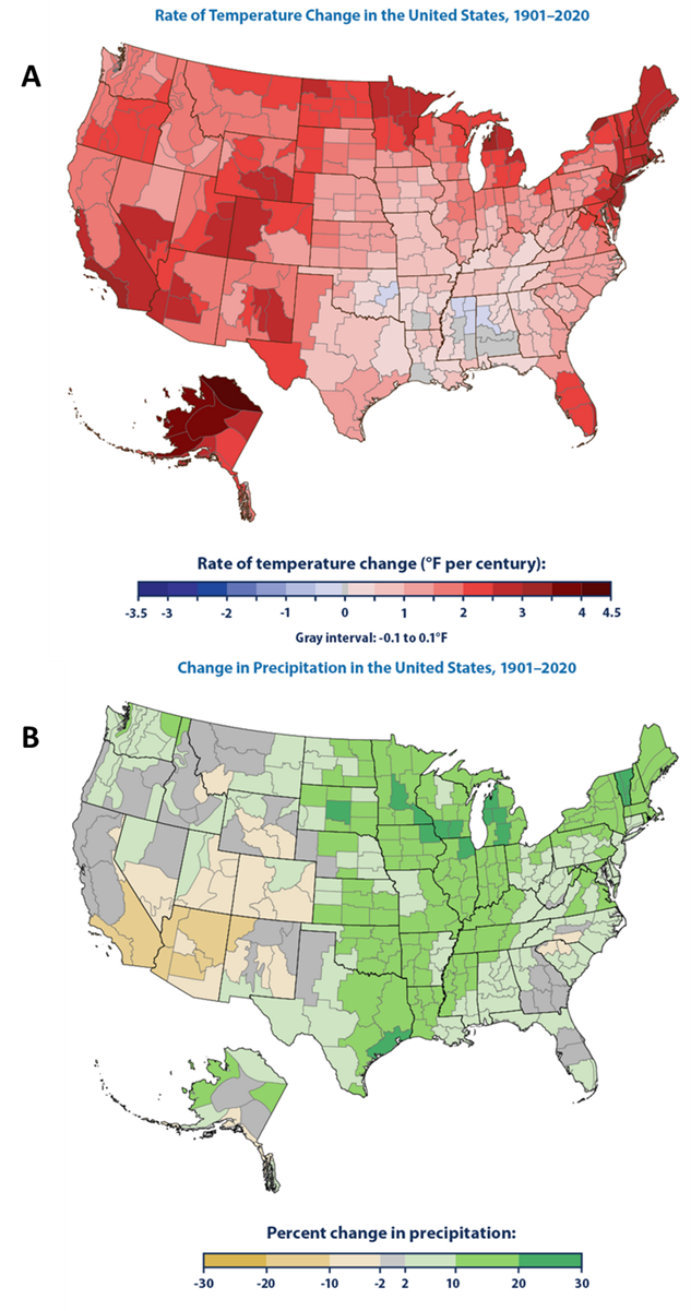
Two of the most fundamental aspects of local climate are its average temperature and precipitation. The increase in global average temperature and the disruptions to the large-scale circulation of ocean and air currents are causing changes to temperature and precipitation at more local scales. These changes are not uniform. For example, since 1901, the average temperature across the contiguous 48 United States has risen at an average rate of 0.09°C (0.16°F) per decade, and precipitation has increased at a rate of 0.51 cm (0.20 inches) per decade.49 But different parts of the United States have been warming much faster than others (Figure 4.10A), and while some regions have been getting wetter, others have been getting drier (Figure 4.10B). A notable example is the southwestern United States, which has been experiencing a prolonged dry period that began at the start of this century. So far, this has been the driest stretch the region has experienced since the late 1500s and the second driest since the year 800.50
These regional differences reflect the unique factors that shape climate at the local scale. For example, Utqiaġvik, Alaska, sits on the coast of the Arctic Ocean and is the most northern US town. Its air temperature is strongly influenced by the abundance of sea ice just offshore. Like elsewhere in the Arctic, the decline in sea ice has caused much more rapid warming in Utqiaġvik than in other parts of the United States. That’s why the US Environmental Protection Agency (EPA) excluded Alaska from its average warming rate statistic (cited above). In fact, the rate of warming has been so transgressive that it triggered the system designed to ensure the integrity of our long-term weather records. At the end of 2017, researchers at the National Oceanic and Atmospheric Administration (NOAA) noticed that the data from the Utqiaġvik station had been flagged as suspicious by an automated algorithm. The algorithm was designed to alert NOAA that a temperature sensor might have broken or the readings may have been affected by some anomalous local event, such as someone moving the sensor next to a warm building—something that happens surprisingly frequently. But the reason wasn’t that someone had moved the sensor, it was that we have been causing the local sea ice to rapidly decline.
Local sea surface temperatures have also been increasing, and just as on land, there is a lot of variation in the response from place to place. Two examples are the cooling trend in the waters off southern Greenland as a result of glacial runoff, and the intensified warming along the eastern coast of North America as a result of the westward deflection of the Gulf Stream describe above. Another example is related to the vertical depth gradient in ocean temperature. Water is a lot warmer at the surface than it is at depth. In general, the transition from warm to cold tends to be more abrupt than gradual. Ocean water tends to be strongly stratified with a layer of relatively warm, oxygen- and nutrient-poor water sitting on top of a much bigger layer of relatively cool, oxygen- and nutrient-rich water.
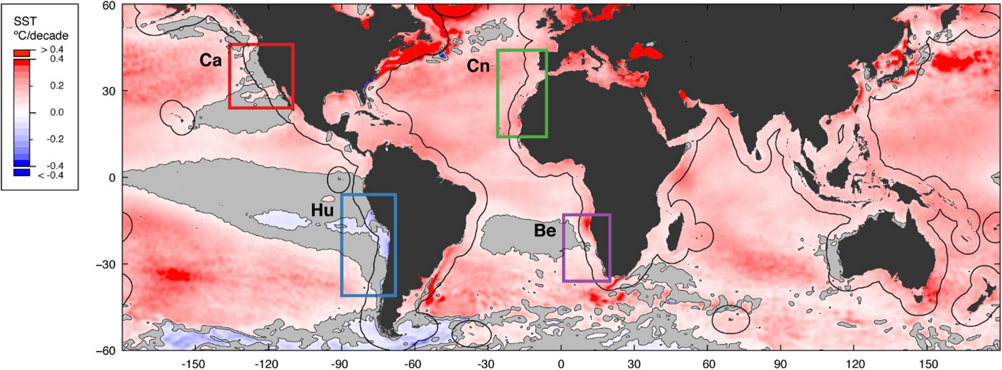
In a few places, strong winds mix up the stratification by displacing surface waters and pulling deeper water to the surface. Important upwelling zones are found along the eastern coastlines of the major ocean basins. In these areas, nutrient- and oxygen-rich deep water mixes with the warm sun-filled surface waters to create ideal conditions for photosynthetic organisms. These eastern boundary upwelling systems are concentrated nodes of primary productivity that support important fisheries. Although eastern boundary upwelling zones cover only about 1% of ocean area, they support one-fifth of the world’s wild fish harvest.51 Increasing global temperature is changing these zones in ways we don’t yet fully understand. On one hand, rising sea surface temperature tends to intensify the stark difference between warm surface water and cold deep water, increasing temperature stratification. At a global scale, increasing stratification could be acting as a positive feedback that further intensifies the warming of surface water.52 However in some eastern upwelling systems the intensity seems to be increasing as the alongshore winds that drive coastal upwelling are themselves intensifying. It's thought that this is due to an increasing temperature gradient between the relatively warm land and the relatively cool ocean.53 In fact, persistent upwelling of cold water in some upwelling zones has buffered these areas from the worst of the ocean warming so far. From 1982 to 2018, the mean rate of ocean warming within the eastern boundary upwelling zones has been half the warming rate outside of the zones, although there is a lot of spatial variation in the strength of the temperature buffering.54 The temperature-buffering effect has been greater in the Pacific than the Atlantic (Fig. 4.11), and upwelling intensification is likely to be more pronounced at higher latitudes than at lower ones.55
Changes to Seasonal Patterns
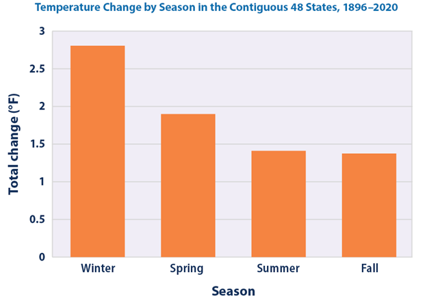
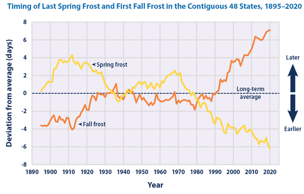
Yearly averages don’t provide a full picture of local climate. Climates also have characteristic seasonal patterns to their conditions. For example, temperature seasonality generally increases as you move from the tropics, where most regions experience little seasonal temperature change, to higher latitudes, where most regions experience pronounced seasonal shifts in temperature. The overall warming of the planet is causing these seasonal temperature patterns to change. In the middle and high latitudes, winters have been getting shorter and summers longer. From 1952 to 2011, summer in the Northern Hemisphere midlatitudes has gotten longer at an average rate of 4.2 days per decade, while winter has gotten shorter by an average of 2.1 days per decade. The changes in duration are reflected in changes to when the seasons start. In 2011, spring started an average of almost 10 days earlier, and winter started an average of 3 days later than it did in 1952.56 Winters are also becoming less cold. For example, since 1896, average winter temperatures across the contiguous 48 United States have increased 1.6°C (2.8°F), and (at least so far) winters have been warming faster than summers (Fig. 4.12). One result of these changes is that the length of time during which temperatures are suitable for plant growth has been generally increasing across the high latitudes. In the contiguous United States, the average frost-free growing season has lengthened by almost two weeks since the start of the twentieth century (Fig. 4.13).
Marine habitats have seasons just as pronounced as those on land. One important seasonal pattern in middle and high latitudes is related to the temperature stratification of the oceans. During the winter, cooling surface waters along with the churning action of winter storms fosters the mixing of relatively nutrient-rich deep water with relatively nutrient-poor surface water. But as surface waters heat up during the summer, the water column gets increasingly stratified with a layer of warm nutrient-poor water at the top and cold nutrient-rich water below. This creates a pronounced seasonal cycle of primary productivity. Phytoplankton at high latitudes peak in abundance during the spring, when the nutrient-rich, well-mixed water of winter combines with the increased light levels and warmth of approaching summer. Many zooplankton that feed on the phytoplankton then peak in early summer, just after the peak in phytoplankton. As I mention above, models suggest (with the exception of the eastern boundary upwelling zones) that warming could cause ocean stratification to become more pronounced and slower to break down at the onset of winter. That would significantly delay and reduce the replenishing flow of nutrients from deep water to the surface, reducing overall marine productivity.57
We have already observed changes in the seasonal abundance patterns of marine organisms, although there is a lot of variation. Some peaks are coming earlier, some later, and others haven’t changed much at all.58 Such uneven patterns can cause organisms (both in the sea and on land) to get out of sync and disrupt the ecological relationships among organisms in a community (see Chap. 5).
More Extreme Conditions
The long-term average of conditions for a particular location is climate. The day-to-day variations that we live our lives through is weather. There is no typical day weather-wise; each day’s weather differs from the long-term average to some extent or another. Still, some days are more unique than others. Extreme deviations from the long-term average conditions are nothing new. There have always been heat waves, droughts, floods, and powerful storms. But we have increasingly strong evidence that Earth’s energy imbalance is increasing both the frequency and intensity of a range of extreme weather events. One reason for this is that as average conditions shift, the likelihood of what were once extreme and rare events also increases. Extreme high temperatures are probably the most straightforward example.
In July 2010, more than 1 million km2 of western Russia was hit be a severe heat wave. Moscow’s temperature reached 38.2°C, the highest ever recorded. Before it was over more than a month later, the heat wave killed an estimated 11,000 people in Moscow alone and spawned massive wildfires across the country. At first, scientists were uncertain about how human climate change may have contributed to the severity of the heat wave. Some pointed out that while the heat wave was nasty, it wasn’t all that extreme relative to past heat waves, and therefore human influence wasn’t a big factor. Others argued that the overall trend of increasing temperatures caused by human climate change had made such an extreme event more likely to happen.
A group of scientists led by Friederike Otto reconciled these two hypotheses with an elegant study.59 They used climate models to predict the probability distribution of heat waves with varying severity. They did this using two models: one that modeled conditions that prevailed during the 1960s, when our climate influence was low, and one that modeled conditions during the 2000s, when our climate influence was high. This allowed them to test the extent to which human influence had altered both the severity and frequency of Russian heat waves. They found, as the previous research had suggested, that the 2010 heat wave wasn’t that much more severe than past heat waves. It was just a couple of degrees warmer than what a heat wave with the same probability of happening would have been like during the 1960s. But their model showed that by making all heat waves just a little bit more severe than they used to be, climate change significantly increased the frequency of the most severe events. Before human-induced climate change, a heat wave that severe would hit Russia about once every 99 years; with human influence, the return time had shrunk to once every 33 years.
The 2010 Russian heat wave wasn’t an isolated event. Globally, heat waves have been getting more frequent and lasting longer. For instance, during the 1960s, major cities in the United States experienced an average of two heat waves per year, and they tended to last about three days; by the 2010s, the heat wave frequency had increased to six per year, and the average duration was about four days.60 We also shouldn’t blithely discount a few degrees of added warmth to a heat wave. At the extreme end, those added few degrees are beginning to generate temperatures that are transgressive, even for a heat wave. In June 2021, the Pacific Northwest experienced a heat wave that shattered previous records. Lytton, British Columbia, reached 49.6°C (121.3°F), the highest temperature ever recorded in Canada. A day later, most of the town was destroyed by a wildfire.61
Portland, Oregon, reached 46.7°C (116°F), giving it a high temperature record greater than that of Houston’s 43°C (109°F). Across both Canada and the United States, the unprecedented heat caused at least 700 deaths. Washington State recorded 78 deaths, more than the total 39 heat-related deaths the state saw during late spring and early summer over the previous six years.62 An early unpublished analysis concluded that human-caused climate change made the 2021 Pacific Northwest heat wave 2°C hotter and 150 times more likely to happen. The heat wave was still extremely rare; the researchers estimated that it was a 1-in-1,000-year event in today’s climate. If we continue to increase global temperature, however, such extreme events will likely become commonplace. The researchers estimated that if we increase global average temperature by 0.8°C warmer than what it was in 2021 (to 2°C above the preindustrial level), a heat wave that severe would occur in the region roughly every 5 to 10 years.63
A range of other factors related to Earth’s changing energy balance also likely contribute to intensifying weather patterns, although we still don’t understand their influence very well. For example, shifts in global air circulation patterns associated with arctic amplification described above have been identified as contributing to the intensity of recent heat waves in Europe and North America.64 A number of feedbacks operating at the local and regional scale seem to play a role.
The ice-albedo feedback contributing to intensified arctic warming is one example. Another is the feedback between soil moisture and air temperature. Soil moisture helps to dampen local air temperature by absorbing solar radiation and evaporating. In regions that are experiencing reduced precipitation during a drought, the declining soil moisture creates a drought-heat wave feedback. With less soil water to evaporate, air temperatures get warmer, which in turn causes even more evaporation of what little soil moisture remains. This feedback likely has intensified the extended period of drought and hot temperatures experienced by the southwestern United States in the early part of the twenty-first century.65
In other regions, the connection between rising temperature and greater evaporation is contributing to more intense rainfall. Rising global temperature has increased atmospheric water vapor, mostly evaporated from the ocean. That water eventually falls back as precipitation, and just like with temperature, the increased baseline amount of water vapor has increased the likelihood of extremely intense rainfall events. On a global scale, the annual maximum daily precipitation increased by 8.5% from 1901 to 2010.66 One specific example of the increasing rainfall intensity was Hurricane Harvey. At the end of August 2017, Hurricane Harvey stalled over southern Texas and dropped an epic amount of rain. In some locations, the eight-day rainfall total exceeded 152 mm (60 inches), more than their normal total annual rainfall. The resulting flooding directly killed 68 people and caused $125 billion in damage.67 Two independent studies concluded that our climate change had caused the rainfall in the storm to be 15% to 38% more than it would have been.6869 The Oldenborgh et al. study estimated that before human-induced climate change, a storm like Harvey would have occurred in the region once every 2,400 years. After our changes to climate, the probability is now one in 800 years.
The success of approaches such as those used by the researchers who studied the 2010 Russian heat wave has spurred a growing area of research called extreme event attribution that tries to figure out the causes of extreme weather events as well as the degree to which climate change played a contributing factor. Since 2011, the Bulletin of the American Meteorological Society has published an annual report that analyzes the causes of extreme weather events during the previous year. Over that period, about 65% of the 131 studies submitted to the report identified a role for climate change, while about 35% found no appreciable effect.70
Spatial Shifts in Climate Zones
One consequence of the changes to local and regional climate described above is that the current geographic distribution of Earth’s major climate zones is shifting (Fig. 4.14). At a broad global scale, the tropics are expanding, and other climate zones are moving poleward. The two poleward edges of Earth’s tropical zone have been expanding at about half a degree of latitude per decade since 1979.71 In climactic terms, the poleward edges of the tropics are where warm air that has risen near the equator descends back to Earth. This has typically been around 30°N and 30°S latitude. Because the descending air has lost much of its moisture, these regions tend to be characterized by warm, arid climates such as the Sonoran Desert of northern Mexico. Partly as a result of tropical edge expansion, the total area of Earth’s terrestrial arid climate zones has increased, even though average global precipitation has also increased. As the tropics expand, other climate types have shifted poleward and contracted. The fastest and most existential changes are happening at the poles, where there is no more room for climate types to spatially shift. This is particularly the case for terrestrial polar and subarctic climate types such as tundra because there is little land surface in northern polar regions above 66°N, and most of the land surface at the southern poles lies under several thousand meters of ice. A similar process is happening vertically as lowland climates expand upslope and alpine climates get squeezed.
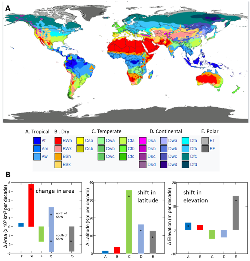
Marine climates are undergoing a similar spatial shift. While temperature and rainfall are the biggest components of climate on land, in the ocean, it is temperature and dissolved oxygen. On land, oxygen availability doesn’t change much unless you go up in elevation; there is more or less as much oxygen in the air of Rio de Janeiro, Brazil, as there is in the air Utqiaġvik, Alaska. Things are different in the ocean, where the abundance of dissolved oxygen is strongly temperature dependent. As ocean temperature increases, the amount of dissolved oxygen it holds decreases. To compound the issue for organisms, ectothermic organisms require more oxygen for their metabolic processes as temperature increases. Many marine organisms have evolved to require a specific range of oxygen availability across a range of specific temperatures in much the same way that terrestrial organisms have evolved to require a specific range of temperature and rainfall. As a result, metabolic suitability partly defines suitable habitat zones and spatial ranges for many marine species. In relative terms, overall metabolic suitability (defined as the ratio of oxygen availability to organism metabolic demand) is tenfold less in the warm oxygen-poor waters of the tropics than in the cold oxygen-rich waters of polar regions.72 Relative metabolic suitability also increases with depth, although to a lesser extent than with latitude. As global temperature rises, the distribution of many marine species will likely contract and shift poleward as water along the equatorward edge of their ranges becomes too low in oxygen to support their increased metabolic demand for it. These contractions could reduce the average metabolic suitability of the ocean by as much as 20% under some predictions.73
4.5 Climate Prediction
Section 4.5: Climate Prediction
I have so far focused on changes that humans have already made to the climate system. These changes are significant, and we have already pushed climate past the clear safe zone under the planetary boundary system described in Chapter 1 (see Section 1.7). Unless we alter how we influence the climate system, these changes will continue until climate has properties and characteristics that are way beyond those that shaped our biological and social evolution. But what does that mean in tangible terms, like how hot and dry the US Southwest will be 30 years from now, or where the best regions for growing wheat will be in 59 years? We need detailed predictions about future climate in order to effectively plan how to adapt to the changes. Even more importantly, we need clear predictions about what future climate will be like in order to make informed decisions about what actions we should take now in order to mitigate the changes and the disruptions they will cause.
Climate Models
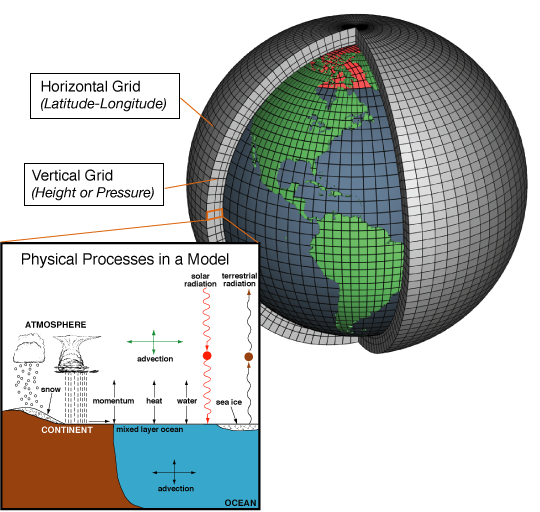
Important tools for making these predictions are mathematical models of Earth’s climate system called general circulation models (GCMs). At a conceptual level, GCMs are more detailed versions of Figure 4.1. But GCMs go beyond Figure 4.1 in several ways. First, they use mathematical equations to explicitly describe the physical and biological processes that govern the various aspects of climate such as how clouds form, how sea ice melts, and how plants absorb CO2. The equations are based on fundamental physical relationships, such as that between temperature and how much water vapor air can hold. Climate models also differ from Figure 4.1 in that they describe the dynamic flow of energy, water, and air across the globe and over time.
The equations describing the flow of air and water are some of the more complex parts of climate models. An example: the set of partial differential Navier-Stokes equations that describe fluid flows have no known exact solution, so they must be approximated numerically. As of 2021, there is still a $1 million prize on offer for anyone who figures out an exact solution to them.74 Climate model equations also incorporate the various feedbacks in the climate system, such as the ice-albedo feedback, and that also greatly complicates the solutions. The other important complicating difference between climate models and Figure 4.1 is that they explicitly model space and time. Most GCMs do this by describing the world as a three-dimensional grid (Fig. 4.15). When GCMs are run, computers solve the physical process equations for each individual grid cube. The results are then passed to neighboring cubes where they are used to update the parameter values, and the equations are solved again. Repeating the process through many time steps creates a dynamic simulation of the Earth System through time. Running GCMs is like building an autonomous robot and then sitting back to watch where the robot goes and what it does. Although the GCMs are constructed using mathematical equations, their collective output over time is far from predictable beforehand. The outputs from all the individual equations that make up GCMs interact across the model’s range of spatial scales and across the time over which the models are run. These interactions produce emergent phenomena—such as how wavy the jet stream over Europe will be on May 3, 2075, or how cloudy the sky over Portland, Oregon, will be on the morning of December 19, 2091—that are not explicitly coded for in the equations. Even if the same exact parameter values are used to start, each simulation run will produce a unique set of results. To account for that variability, model predictions are usually reported as the average results from multiple model runs.
Details such as how cloudy it is over a particular region on a particular day sounds more like weather than climate, and indeed versions of GCMs have been developed specifically for weather forecasting. The big difference between the weather and climate versions of these models is the spatial and temporal resolution they are focused on. Weather forecast models are optimized to give highly accurate predictions at small spatial scales over short periods. The model parameters are constantly being updated and rerun with new real data from weather stations. The forecasts you get on your weather app are made from models that were probably run just a few hours before. In contrast, climate models are optimized to predict global-scale properties such as the global average surface temperature decades and even centuries into the future. Climate models aren’t good at predicting weather events: you can’t use one to predict if it will rain on your wedding day two years from now. But you could use one to predict what the global average surface temperature will be on your wedding, or on your fiftieth wedding anniversary, or on the wedding day of one of your great-grandkids.
One big constraint in the design of both weather and climate models is the immense computational power needed to run the programs. In fact, the quest to build supercomputers with ever more prodigious computational power has been driven in no small measure by the need for more accurate and high-resolution climate and weather models. That quest has been paying off. Just a few years ago, the highest-resolution GCMs had grid sizes with surface footprints of 250-600 km2. Today, some GCMs use grid sizes with footprints of about 5–11 km2. That is similar to the resolution used by many weather prediction models, and it is high enough to depict medium-scale phenomena, such as the eddies that bud off the Gulf Stream and the formation of tropical cyclones, in realistic detail. Climate models are even being developed that have 1-km2 resolution.75 The increased computation power of supercomputers has also allowed us to build GCMs that include more details of the climate system, and we have been able to provide those details as our understanding of the climate system has grown. Current models now include such details as the chemical reactions of greenhouse gasses in the atmosphere, the photosynthetic dynamics of vegetation, and the working of the thermohaline circulation system.
Researchers have developed several different GCMs. Each one takes a slightly different approach to things such as what climate processes it includes, what spatial scales it covers, what assumptions it makes, and the details of how it processes the calculations. Each GCM has its own idiosyncratic tendencies and aspects of the climate system that it is particularly good or bad at simulating. Researchers sometimes chose a particular model that is well suited to the question they are asking, but in many cases, there is no obvious way of deciding which model is best. One commonly used approach is simply not to make a decision and instead run a range of different GCMs using the same parameter values. Researchers then statistically combine the outputs into one ensemble simulation.76 Using ensemble model results is like coming up with a consensus opinion from a room full of experts.
Just as with any prognostication, the predictions made by climate models involve uncertainty. We can’t, of course, directly test distant future predictions against the real outcomes, but we can use other approaches to help evaluate and quantify the uncertainty in GCM predictions. One approach is to measure the variability in outputs between model runs and across different GCMs. Modelers can also assess how sensitive the model results are to certain assumptions, parameter values, or model components. Predictions of climate traits that depend heavily on parameters that we have sketchy data for or on processes that we still don’t understand very well have a higher degree of uncertainty. Another approach is to run the models backward in time and evaluate the model results against past climate records. Finally, we have been constructing sophisticated GCMs for several decades now, which is just enough time to get a sense of how well they did at predicting future climate in the years after they were published. One study did just that by comparing how several GCMs published between the early 1970s and the 2000s did at predicting global temperature. In general, the models were accurate (Fig. 4.16). As with any model, however, the accuracy of GCMs depends on the accuracy of the key climate drivers used as input parameters for the models. But it is difficult to decide what values to use to parametrize GCMs because we are continuing to dramatically change the key drivers, most notably the concentration of CO2 in the atmosphere. When they were first published, many of the 17 GCMs used assumptions about future atmospheric CO2 that turned out to be a bit off. When the researchers parameterized the models using the actual CO2 values, their accuracy improved even further.77
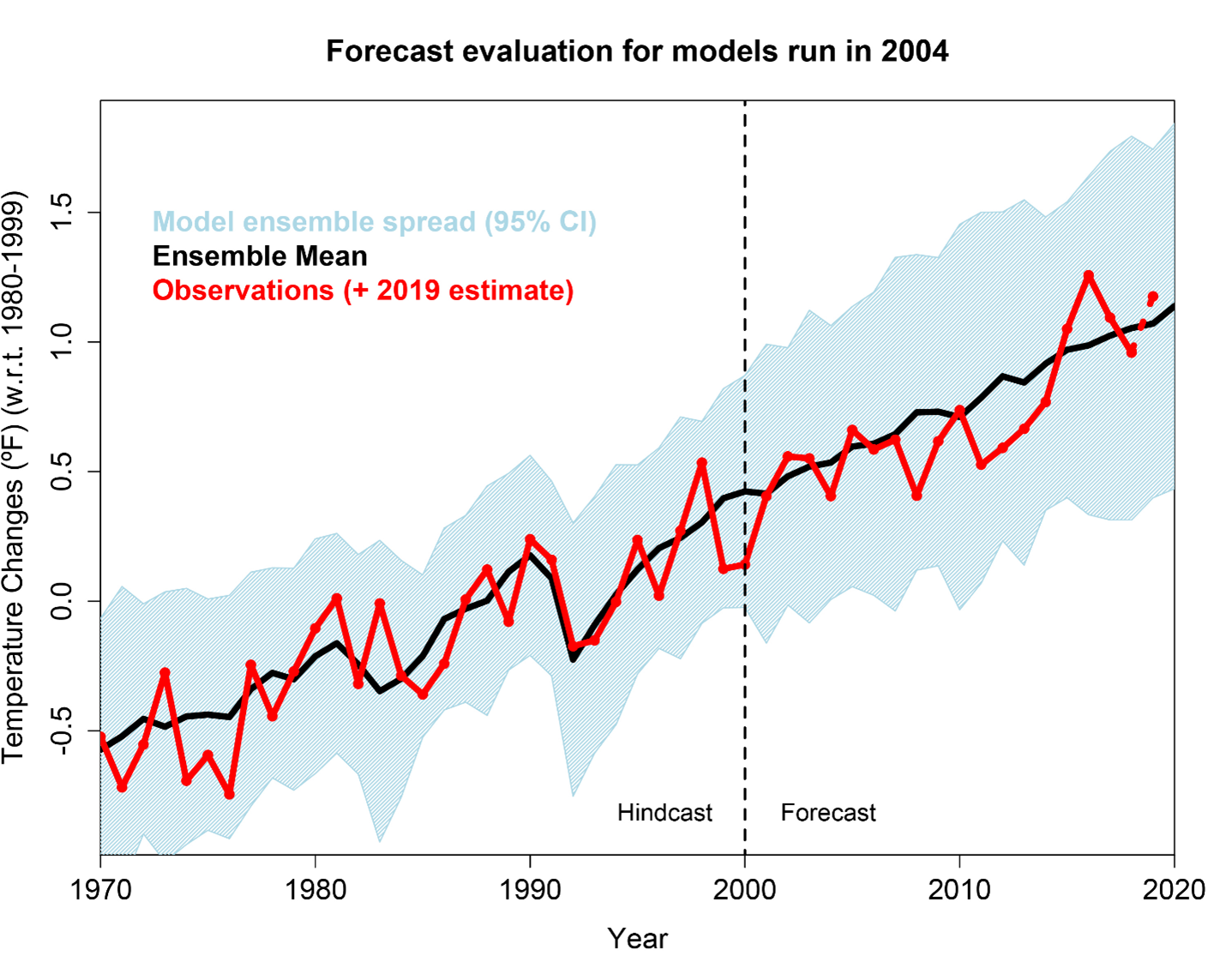
In general, the uncertainty of GCM predictions increases the further out in time we ask the models to make predictions for. That is partly because our ability to predict how much we will change the underlying climate drivers in the distant future is so poor. That brings up an important question. If the accuracy of GCMs is so dependent on the future value of climate drivers for which we are uncertain, what use are they as predictive tools? The answer is to view the predictions made by GCMs not as predictions of what will happen, but instead as potential scenarios that would likely happen based on our climate actions.
Potential Future Scenarios
Climate models are remarkable tools, but in order to work as predictors of future climate, they need to account for the ways that we are changing Earth’s climate system. How much more fossil fuels will we burn? How many forests will we convert to agriculture? How many wetlands will we drain? Predicting those things is way more difficult than constructing accurate physical models of the climate system. While fields such as economics, sociology, and political science have made great strides in describing the factors that shape our societies and political decisions, they struggle to make predictions. Predicting the unemployment rate or the outcome of an election a year out is fraught with uncertainty. Confidently predicting what our global actions related to Earth’s climate will be 30 or 50 years from now is nearly impossible.
To get around that difficulty, we have taken a slightly different approach. Instead of predicting what our climate actions will be, we have developed a wide range of scenarios that describe approaches and actions that we could take. One set of scenarios that have been developed are called shared socioeconomic pathways (Table 4.2). The five scenarios are different plausible plots of how our society and economy could develop over this century. For instance, in one plot arc (Taking the Green Road) we gradually move toward more sustainable economic systems that emphasize collective human well-being and global cooperation. An alternative plot arc (A Road Divided) involves growing social inequities and a widening division between rich and poor. A notable aspect of the shared socioeconomic pathways is that they do not explicitly describe any concerted policy efforts to reduce our climate impact. None of the scenarios, for instance, envisions a global tax on greenhouse gas emissions. The scenarios are meant to describe different baseline ways our global society could develop in the absence of comprehensive climate policy. In that sense, all five shared socioeconomic pathways are business as usual scenarios.
| Future scenarios; each scenario is a small table block, with scenario code (SSP 1) and Description |
|---|
| SSP 1. Sustainability – Taking the Green Road |
| The world shifts gradually, but pervasively, toward a more sustainable path, emphasizing more inclusive development that respects perceived environmental boundaries. Management of the global commons slowly improves, educational and health investments accelerate the demographic transition, and the emphasis on economic growth shifts toward a broader emphasis on human well-being. Driven by an increasing commitment to achieving development goals, inequality is reduced both across and within countries. Consumption is oriented toward low material growth and lower resource and energy intensity. |
| SSP 2. Middle of the Road |
| The world follows a path in which social, economic, and technological trends do not shift markedly from historical patterns. Development and income growth proceeds unevenly, with some countries making relatively good progress while others fall short of expectations. Global and national institutions work toward but make slow progress in achieving sustainable development goals. Environmental systems experience degradation, although there are some improvements and overall the intensity of resource and energy use declines. Global population growth is moderate and levels off in the second half of the century. Income inequality persists or improves only slowly and challenges to reducing vulnerability to societal and environmental changes remain. |
| SSP 3. Regional Rivalry – A Rocky Road |
| A resurgent nationalism, concerns about competitiveness and security, and regional conflicts push countries to increasingly focus on domestic or, at most, regional issues. Policies shift over time to become increasingly oriented toward national and regional security issues. Countries focus on achieving energy and food security goals within their own regions at the expense of broader-based development. Investments in education and technological development decline. Economic development is slow, consumption is material-intensive, and inequalities persist or worsen over time. Population growth is low in industrialized and high in developing countries. A low international priority for addressing environmental concerns leads to strong environmental degradation in some regions. |
| SSP 4. Inequality – A Road Divided |
| Highly unequal investments in human capital, combined with increasing disparities in economic opportunity and political power, lead to increasing inequalities and stratification both across and within countries. Over time, a gap widens between an internationally-connected society that contributes to knowledge- and capital-intensive sectors of the global economy, and a fragmented collection of lower-income, poorly educated societies that work in a labor intensive, low-tech economy. Social cohesion degrades and conflict and unrest become increasingly common. Technology development is high in the high-tech economy and sectors. The globally connected energy sector diversifies, with investments in both carbon-intensive fuels like coal and unconventional oil, but also low-carbon energy sources. Environmental policies focus on local issues around middle and high income areas. |
| SSP 5. Fossil-fueled Development – Taking the Highway |
| This world places increasing faith in competitive markets, innovation and participatory societies to produce rapid technological progress and development of human capital as the path to sustainable development. Global markets are increasingly integrated. There are also strong investments in health, education, and institutions to enhance human and social capital. At the same time, the push for economic and social development is coupled with the exploitation of abundant fossil fuel resources and the adoption of resource and energy intensive lifestyles around the world. All these factors lead to rapid growth of the global economy, while global population peaks and declines in the 21st century. Local environmental problems like air pollution are successfully managed. There is faith in the ability to effectively manage social and ecological systems, including by geo-engineering if necessary. |
The different societal trajectories do have different climate impacts, however. For instance, the Green Road pathway envisions a world where we gradually reduce our energy and material use intensity, which should reduce our greenhouse gas emissions. The different pathways also envision different levels of human well-being, and as such they are framed in terms of the degree to which we manage to achieve a safe and just space for humanity—the Anthropocene doughnut envisioned by Kate Raworth described in Chapter 1 (see 1.17). For instance, the Green Road and Taking the Highway scenarios both envision a world with high and equitable levels of human well-being. In Taking the Highway, however, we achieve that well-being through intensive energy use, which will presumably result in significantly more Earth System changes. Achieving well-being goals in the face of those changes would require us to invent and implement significant strategies and technologies for adapting to those changes. It is an open question whether we will be able to do that.
We can use our understanding of economics and sociology (augmented with some educated guesses) to estimate how the different socioeconomic scenarios will influence Earth’s energy balance in terms of radiative forcing. But as I said at the start of this section, that isn’t always straightforward. A parallel and simpler approach to building future scenarios is to focus on the range of radiative forcing that could conceivably happen and not worry too much about explicitly describing the socioeconomic narratives that create those forcings. The standard set of these types of scenarios are called representative concentration pathways (RCPs). In addition to being a lot easier to construct, a benefit of this approach is that we can easily frame scenarios as potential goals for us to achieve without having to prescribe any particular way of achieving the goal. For instance, we could ask what climate will be like if we somehow manage to keep the end-of-century radiative forcing just slightly above what it is now.
Figure 4.17 describes the estimated radiative forcing and the resulting mean global temperature for several future scenarios. These scenarios depicted in the figure are part of a standard set that have been adopted by the Intergovernmental Panel on Climate Change (IPCC) in its fifth and sixth assessment reports.78 The high and low outcomes predicted by the shared socioeconomic scenarios are in gray, while a range of representative concentration pathways are the colored lines. Note that as of 2020, we have already increased global temperature by 1.2°C. All the scenarios that keep future global temperature below 2°C require substantial reductions in net CO2 emissions.
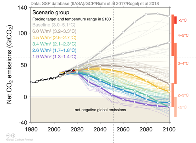
Climate modelers can use the greenhouse gas emissions and land use changes described by the different scenarios as input parameters for global circulation models. The model outputs can then be used to estimate future climate in more meaningful detail than simply global mean temperature. Figure 4.18 describes estimated changes to the amount of annual rainfall in the heaviest 1% of events across the United States under two RCP scenarios. Under both scenarios, many regions will experience more of their annual rainfall in the form of heavy rain events, continuing a trend that has been observed over the past century. The shift to more extreme rain events is greater under RCP 8.5 than RCP 4.5.
RCP 8.5 assumes that we will increase radiative forcing by 8.5 W m-2 by the end of the century. That scenario is a bit controversial because in order to attain it, we would have to keep up the accelerating pace of greenhouse gas emissions that we had been on since 1950 for most of this century, something that many researchers think is unrealistic.79 They point to changes such as the increasing efficiency of industrial processes and reductions in the use of coal as a fuel source that have been occurring mostly for economic reasons, but that nevertheless will reduce the growth of our greenhouse gas emissions. RCP 8.5 is something like a worst-case scenario that requires some pessimistic assumptions. In contrast, RCP 4.5 is a relatively optimistic scenario that would require us to significantly curb our greenhouse gas emissions by the middle of the century. Note that RCP 4.5 requires a greater reduction in greenhouse gas emissions than that envisioned by the green road baseline shared socioeconomic pathway, but it still results in significant increases to rainfall intensity, particularly in the Northeast and Pacific Northwest.
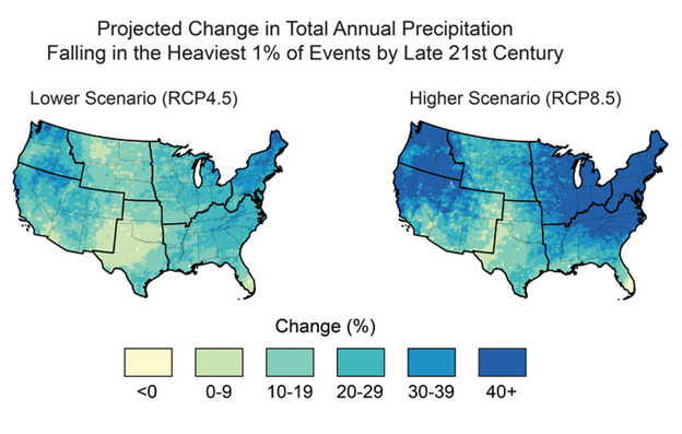
Outputs such as those in Figure 4.18 are important decision-making tools. At one level, the forecasts can be used as planning guides. For instance, Figure 4.18 suggests that the US Northeast is likely to suffer significantly greater future flooding risk even under a middle-of-the-road climate scenario such as RCP 4.5. Prudent local and regional governments would use that information to update their emergency response planning and to develop adaptation strategies such as changes to building and zoning codes. Another use of climate projections is to better inform decisions about what actions we should take to mitigate our climate impact. There are many immediate disincentives to reducing our climate impact, such as the upfront costs of transitioning to carbon-neutral energy sources. But there are also many costs to not taking climate action. Climate forecasts help to quantitatively frame the potential costs. For example, as radiative forcing increases, climate models predict an increased frequency of extreme temperature events such as heat waves.
The more frequent extreme temperature events under RCP 8.5 are projected to result in more than 9,000 additional premature deaths per year across 49 major US cities by the end of the century. The financial costs associated with those deaths is projected to be $140 billion (in 2015 dollars). In contrast, more than half of these deaths could be avoided and the financial cost would be $60 billion if we follow the RCP 4.5 scenario (Fig. 4.19). Those estimates assume that we don’t take measures to adapt to the new climate conditions, such as increasing our use of air conditioning. Many of those potential adaptation strategies have their own costs, of course. Higher global temperatures are likely to drive up electricity costs by increasing energy demand to power air conditioning and by increasing the costs of power generation. By 2040, US residential and commercial electricity expenditures are projected to increase by 6% to 18% under RCP 8.5 and by 4% to 15% under RCP 4.5. By the end of the century, average annual energy expenditures under RCP 8.5 are projected to increase by an estimated $32 to $87 billion (in 2013 dollars; US Global Change Research Program, 2018). More broadly, climate change will alter ecosystems in a wide variety of ways, and those changes will affect the ecosystem services that we depend on to support our society and well-being. I provide a brief overview of some of the changes that have already happened in Chapter 5.
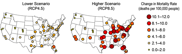
4.6 Limiting Our Climate Impact
Section 4.6: Limiting Our Climate Impact
In 2015, representatives from 196 nations signed a legally binding treaty known as the Paris Agreement that committed them to limit global temperature increase compared to preindustrial levels to well below 2°C, preferably to 1.5°C. The 1.5°C goal still leaves us within the zone of elevated and uncertain risks for humanity as defined by the planetary boundary system (see Section 1.7). Agreeing to a goal that still involved societal risks reflected the practical reality that we had already increased global temperature by about 1°C (1.2°C as of 2020), and that at the time of the Paris Agreement, the rate at which we were adding greenhouse gasses to the atmosphere was still accelerating. The 1.5°C target was seen as an ambitious but attainable goal.
Achieving the goal requires countries to take immediate steps to halt the increase in greenhouse gas emissions and to achieve a climate-neutral world by midcentury. That future is represented by RCP 1.9 in Figure 4.17. Each country in the agreement is required to develop plans for their contribution toward meeting that goal known as nationally determined contributions (NDCs). The United States submitted a revised version of its plan in April 2021 after it rejoined the Paris Agreement (it had briefly left the agreement in 2019 under President Trump). In its 2021 plan, the United States set an economy-wide target of reducing its net greenhouse gas emissions by 50% to 52% below 2005 levels by 2030.80
Countries can achieve their Paris Agreement commitments using a wide variety of approaches, and there is no shortage of discussion, argument, and consternation about what the best approaches are for any given country. I won’t explore the potential approaches or the debate related to them in any detail, although I will mention a few specific strategies in some of the subsequent chapters. Here, I will just briefly mention the three broad conceptual ways to reduce our climate impact.
Reduce Greenhouse Gas Emissions
Probably the most direct and technologically straightforward approach to mitigating our climate impact is to reduce the amount of greenhouse gasses being transferred to the atmosphere. That is easier said than done, given that our society is still largely based on burning fossil fuels and on intensive agricultural practices. But the hurdles to reducing our emissions are more social and political than they are technical. We have developed an array of alternative options for generating energy, including wind, solar, hydroelectric, nuclear, and geothermal. We have also started to develop strategies for reducing the climate impact of our food and agricultural systems. For sure, each of the alternatives have downsides that include their own impacts to Earth’s ecosystems.81 But the biggest immediate hurdle to implementing these alternatives has been the various financial costs involved in transitioning to them.
In Section 2.5, I discussed how not accounting for the value of ecosystem services (such as climate regulation) can produce an incomplete accounting of the true costs and benefits of reducing biodiversity. A similar situation exists for greenhouse gas emissions. The true ecological and social costs of greenhouse gas emissions are not fully accounted for by the market price of a gallon of gas, a train full of coal, or a bushel of corn. We can use approaches similar to the ecosystem service valuation approaches that I describe in Section 2.5 to estimate the direct economic damages caused by greenhouse gas emissions from things such as excess deaths during more frequent and extreme heat waves.
A standard metric is the social cost of carbon, which is a dollar estimate of the damages that would result from emitting one additional tonne of greenhouse gases into the atmosphere. In 2021, the official US government estimate of the social cost of carbon was $51 per tonne, a value that will likely increase as the estimation is revised to better account for the inequitable distribution of risks across society and on future generations.82 A number of strategies have been proposed for using that cost estimate to incentivize reductions in greenhouse gas emissions. One of the most frequently discussed—and potentially most effective—is taxing fossil fuel use and/or carbon emissions.
Perhaps because taxes inherently make people grumble, carbon taxes have not yet been widely adopted. In 2016 and again in 2018, voters in Washington State rejected carbon tax initiatives, and in 2018, widespread protests erupted across France in part because of a planned climate-related increase to the gas tax. How carbon taxes are viewed depends on who people perceive as bearing the cost and reaping the benefit of the tax. Gas taxes, for instance, are often viewed as unfairly placing the burden of climate mitigation on the middle class and poor. Designs that more equitably share carbon tax burdens and revenues can gain broad support.83
Our society and economy can also potentially reduce greenhouse gas emissions even without the extra push of public policy. One way this can happen is through the drivers of technological innovation and globalized markets that spurred the Great Acceleration in greenhouse gas emissions in the first place. Rapid advances in renewable energy technology are dramatically driving down their cost to the point that they are increasingly the cheapest source of energy, even compared to fossil fuels. There has also been a surge of global capital into renewable-energy-associated companies such as Tesla that is spurring additional research and development and making renewable energy production and delivery a greater part of the global economy. These rapid changes are already beginning to transform our energy use.
On April 21, 2017, Great Britain went the entire day without burning coal to generate electricity. That was the first time that had happened since the start of the agro-industrial revolution in the 1800s. While most of Britain’s energy that day was still generated using other less CO2-intensive fossil fuels such as natural gas, the milestone still seemed to mark the beginning of the end of our love affair with fossil fuels. Importantly, a broad swath of humanity now recognizes the climate threat that we have created, and there is a broad consensus that we need to take action. A survey of Facebook users conducted across 30 countries in 2021 found overwhelming support for participation in the Paris Agreement, and large majorities within each country think that climate change should be a “high” or “very high” priority for their governments.84 As a result, the historical dichotomy between immediate economic interests based on fossil fuels and the desire to avert future climate change is disappearing. In 2021, a broad coalition of shareholders in the giant oil company Exxon Mobil were able to install three directors on the board with the goal of pushing the company to take more substantive action to help reduce its climate impact.85
Enhance Climate-Related Ecosystem Services
Despite the promising signs, many people fear that our actions to reduce greenhouse gas emissions are currently still too little and too late to avert levels of climate change that will cause severe disruption to our society. Many people argue that any hope of meeting the goals of the Paris Agreement will require us to use a variety of additional methods to adjust Earth’s energy balance.86
A broad approach is to sequester CO2 out of the atmosphere. One way of doing that is to restore the capacity of terrestrial ecosystems to absorb greenhouse gasses. Restoration has a lot of potential because vegetation and soil are significant storage sinks for atmospheric CO2 (Fig. 4.5). For example, over the years 2001–2019, just the world’s forests removed about 7.6 Gt of greenhouse gasses per year from the atmosphere measured in CO2 equivalent (CO2e). But we have diminished the size of terrestrial carbon reservoirs by altering the biological composition and abiotic conditions of landscapes through activities such as draining wetlands, setting annual fires for agriculture, and raising methane-belching cattle (see Chap. 3). Our land use practices were historically the main source of our greenhouse gas emissions, and they continue to be a significant source of current emissions even as the dominant source shifted to fossil fuel burning (Fig. 4.4). For instance, the net 7.6 Gt of CO2e sequestered each year by the world’s forests is the balance of gross greenhouse gas uptake (15.6 Gt CO2e yr−1) and gross emissions (8.1 ± 2.5 Gt CO2e yr−1) caused by deforestation and other practices such as setting wildfires.87 Ongoing land use change in the remaining forests of the Amazon and Southeast Asia is a particular concern. One study that comprehensively assessed how land use change in the Amazon Basin has altered the net flux of greenhouse gasses concluded that the Amazon has likely stopped being a net sink of greenhouses gasses and is now a net exporter.88
Enhancing the capacity of terrestrial ecosystems to sequester greenhouse gasses seems as enticingly simple as planting more trees. Indeed, several global climate initiatives such as the World Economic Forum’s One Trillion Trees Campaign are framed around that tangible goal. Simply planting trees can give a false sense of accomplishment, however. Tree planting often does not involve changing other greenhouse-gas-generating land use activities such as draining wetlands or frequent burning, so the net result in terms of sequestering greenhouse gasses is negligible.89 To develop the most effective climate mitigation tools, we need to think more comprehensively about how to adjust ecosystem traits and processes in ways that will enhance net greenhouse gas sequestration. The carbon sequestration that results from restoring wetlands in the Sacramento–San Joaquin River Delta mentioned in Section 3.4 is one example. A broad ecosystem approach also has the additional benefit of conserving biodiversity and enhancing a wider range of ecosystem services. Some of those ecosystem services can help us adapt to or indirectly mitigate some of the damages caused by climate change. The storm protection services provided by coastal wetlands are an example. I explore approaches for enhancing the ecological function of landscapes in more detail in Chapters 7 and 9.
Climate Engineering
We can also pull CO2 out of the atmosphere ourselves using mechanical and chemical means. There are a variety of technologies that are being developed to do this that are loosely called direct air capture. For example, a company called Carbon Engineering has built a prototype plant in Squamish, British Columbia, that uses chemical processes to convert atmospheric CO2 into calcium carbonate.90 The process is a greatly sped-up version of the carbonation process that naturally happens in concrete, described in equation (4.8). In Carbon Engineering’s prototype, the calcium carbonate is then converted back into pure CO2. The CO2 is easier to transport to locations that are suited for long-term storage.91
The main options for storage include injecting the CO2 into deep, impermeable rocks and sediments as well as into reactive geologic formations that have ideal conditions for catalyzing carbonation and mineralization processes.92 At a carbon storage site in Iceland that has a particularly favorable geology, it takes about two years for 95% of the injected CO2 to be mineralized.93 The source of the injected CO2 at that Iceland site comes from a related approach called carbon capture and storage. Instead of capturing the CO2 from the atmosphere, carbon capture and storage diverts CO2 that would normally be released to the atmosphere as a by-product of industrial processes.
Using current technology, a carbon capture system set up at a large coal-fired power plant can capture at least 800,000 tonnes of CO2 per year.94 Both direct air capture and carbon capture and storage involve emerging technologies that have only recently gotten around some of the basic technical hurdles to implementation, and there are still some technical challenges and concerns. For instance, injecting CO2 into geologic storage currently requires a considerable amount of water and can lead to groundwater pollution.95 Another issue is the considerable financial cost of building carbon capture systems at a sufficient scale to have an impact.
We can also do climate engineering by focusing on the incoming solar radiation part of the energy budget. Solar geoengineering would attempt to reflect more of the incoming solar radiation back to space before it can transfer energy to Earth. Some seemingly far-out plans call for creating massive sunshades and mirrors in space. More feasible and researched approaches involve injecting light-scattering aerosols into the upper atmosphere and brightening ocean clouds by seeding them with salt. One use of these technologies could be to mitigate temperature increases in particularly temperature-sensitive ecosystems such as large coral reef systems.96 These technologies are still in their infancy, with a host of conceptual and technical problems to overcome. There are also a range of political and ethical concerns. For instance, what happens if the aerosols one country pumps into the atmosphere cause a cold-induced crop failure or damaging storm in another country? Because of these concerns, many scientists, such as the Union of Concerned Scientists, currently oppose solar geoengineering altogether. Still other scientists believe that the risks can be managed, and that they are certainly less than the risks associated with our current trajectory of warming the planet.97
4.7 A Word in Defense of Science
Section 4.7: A Word in Defense of Science
Just at the time when we could perhaps use science the most, many folks seem to have lost faith in it. Skepticism of science and technology is certainly not new, nor is it unjustified. Science suffers from the same racism, sexism, biases, pettiness, nationalism, and parochialism that exists in our broader society. There is no shortage of examples where flawed science has helped to spread hatred or caused profound misery. Examples are the forced sterilizations, racist economic policies, and genocides that have been partly justified using science.98 Scientists often fail to fully anticipate and explain the societal implications of new knowledge, and their hubris can lead them to downplay their uncertainty and lack of understanding. Upon the development of the first chemical pesticides, for instance, scientists did a poor job of communicating the potential risks of their use or the degree to which they did not yet fully understand what the risks were.
Despite its imperfection, science is the best tool we have yet devised for helping us to transcend our flaws and limitations as people. The scientific method is based on skepticism and questioning assumptions. Many of our most profound advances in knowledge started when a few initially lonely individuals questioned the scientific consensus and orthodoxy of the time. The process is slow, meandering, and often cruel to the individual questioners. One example is our understanding of plate tectonics. The basic idea for plate tectonics was first proposed in 1912 by the German scientist Alfred Wegener. It was met with scathing criticism and ridicule that was not so subtly tinged with anti-German bigotry. For decades, the idea was treated as a cautionary parable told by old geology professors to their students in order to dissuade them from following a wrongheaded path to scientific oblivion. It wasn’t until the 1960s (long after Wegener’s death) that a new generation of geologists began accumulating evidence that eventually made a convincing case for plate tectonics.99 However meandering, cases such as Wegener’s ultimately prove the inherent value of the scientific process, where relentless testing of ideas against evidence eventually sifts away the poor ideas and elevates the good ones, producing an incrementally evolving body of knowledge.
That incremental scientific process has helped us understand how Earth’s climate system operates and how we are altering it. That is perhaps one of our greatest achievements as a species. It is at least equal to our other great scientific and technological feats, such as the germ theory of disease, the DNA model of heredity, and our visits to the moon. But more than those other accomplishments, the evidence that we are altering climate has helped to reshape how we view ourselves and our relationship to the planet we call home. It is appropriately a millennial accomplishment that required a social community of scientists from different backgrounds and disciplines sharing information, crowd sourcing data, and communicating their findings to laypeople in accessible ways. It has also been an inherently practical pursuit. Scientists are often accused of studying esoteric subjects that are seemingly far removed from the struggles of our daily lives. Not so with climate scientists. They have tackled a most fundamental and practical question: How happy will we and future generations be if we continue on our current path of energy use?
Our understanding is not complete, and there are considerable uncertainties about the details of the vastly complex climate system. But those uncertain details do not affect the fundamental conclusion that we are profoundly altering the system. In fact, the very certainty that we have in that conclusion rests on a detailed and comprehensive accounting of where the knowledge gaps still exist. The error bars on the radiative forcing estimates in Figure 4.2 and the spaghetti of different emission pathways in Figure 4.17 are just a couple examples of the ways scientists are explicitly accounting for and describing our lack of knowledge. Many folks have used those marginal uncertainties as an excuse to abdicate their leadership and even to question the usefulness of science altogether. In 2017, Scott Pruitt, the head of the US Environmental Protection Agency under President Trump, was asked whether he believes that “CO2 is the primary control knob for climate.” He answered:
No, I think that measuring with precision human activity on the climate is something very challenging to do, and there’s tremendous disagreement about the degree of impact . . . So no, I would not agree that it’s a primary contributor to the global warming that we see. But we don’t know that yet. . . . We need to continue the debate and continue the review and the analysis.100
Also that year, the EPA’s webpages devoted to climate science disappeared for a time. The fear that data and information about climate science collected by the EPA and other US agencies was disappearing prompted a frenzied global download onto archival servers akin to the transcription of ancient texts by monks as the Roman Empire collapsed.101 The webpages eventually returned, and the administration released the Fourth National Climate Assessment, a congressionally mandated report compiled by US government scientists (see the Additional Resources). The report was released in spite of the administration’s efforts to derail it, however, and after its release, administration officials tried to discredit it. President Trump simply said, “I don’t believe it."102
That is a profoundly dangerous view. Scientists have given us a body of detailed and explicit knowledge that we can use to inform our decisions about what comes next. There are no easy solutions, not the least because politicians and governments must balance a range of competing interests and goals among their constituents. We must struggle with some weighty questions. Is there a way to minimize the near-term disruption to our present economy as well as the negative climate consequences endured by future generations? What exactly are those consequences going to be? What will be the economic, social, and ecological costs of continuing as we have been? Is solar geoengineering a good idea? We need science to help answer those and myriad other questions we haven’t thought of yet.
Chapter Summary
Parts per Million 451
Earth’s climate is generated by the interaction of solar energy with the physical and biological components of the Earth System. We are radically altering those interactions and as a result are radically altering Earth’s climate. Our increasingly detailed understanding of how the climate system works and how we are changing it provides the information needed to mitigate and plan for these changes.
- Key climate attributes such as temperature reflect the rate at which energy enters and leaves the earth system (Figure 4.1).
- A number of factors (climate drivers) influence Earth’s energy budget. Among the most important are the abundance of greenhouse gasses in the atmosphere (Figure 4.2)
- We have increased the abundance of greenhouse gasses in the atmosphere, primarily by altering the global carbon cycle (Figure 4.4), which in turn has increased global temperature (Figures 4.6, 4.7)
- The retained energy has also altered other aspects of the climate system such as patterns of ocean and atmosphere circulation (Figures 4.9, 4.11), local average temperature and rainfall (Figure 4.10), seasonal patterns, (Figures 4.12, 4.13), the frequency and intensity of extreme weather events such as heat waves, and the spatial location of climate zones (Figure 4.14)
- We have developed detailed mathematical models of the climate system called general circulation models (Figure 4.15). We also have developed social-economic models that describe different potential scenarios for how we might influence climate drivers in the future (Figure 4.17). We can combine the two types of models to make predictions about the future climate we will create based on what activities we choose to engage in (Figure 4.18, 4.19)
Additional Resources
- If you couldn’t get through this chapter, watch this! https://youtu.be/n4e5UPu1co0
- Primo Levi was a chemist and writer best known for his works about surviving the Holocaust. His book The Periodic Table is more a memoir than a chemistry text. But the last chapter, titled “Carbon,” is a far better description of the carbon cycle than is found in any textbook: The Periodic Table, translated by R. Rosenthal (New York: Schocken, 1984), 130.
- In 1990, the Congress mandated the US Global Change Research Program to coordinate the government’s scientific research related to climate change. Every four years, they are required to issue a report that summarizes our current knowledge, called the National Climate Assessment. The assessments provide a detailed yet accessible summary of our understanding of climate change and its impacts focused on the United States. The most recent report is the two-volume fourth assessment. The fifth assessment is due in 2023.
- Climate Science Special Report, Vol. 1. Edited by D.J. Weubbles, D.W. Fahey, K.A. Hibbles, D.J. Dokken, B.C. Stewart, and T.K. Maycock. (Washington, DC: US Global Change Research Program, 2017). https://science2017.globalchange.gov/
- Impacts, Risks, and Adaptation in the United States: Fourth National Climate Assessment, Vol. 2. Edited by D.R. Reidmiller, C.W. Avery, K.E. Easterling, K.E. Kunkel, K.L.M. Lewis, T.K. Maycock, and B.C. Stewart (Washington, DC: US Global Change Research Program, 2018). https://nca2018.globalchange.gov/
- Find out how much carbon dioxide is in the atmosphere today: https://www.co2.Earth/
- Climate scientist Gavin Schmidt gives a great TED Talk about how climate models are developed and what they can tell us: https://youtu.be/JrJJxn-gCdo.
References
6Archer, D., 2011. Global Warming: Understanding the Forecast. New York: John Wiley & Sons.
35Arctic Monitoring and Assessment Programme, 2021. Arctic Climate Change Update 2021: Key Trends and Impacts. Summary for Policy-Makers. Oslo: Arctic Monitoring and Assessment Programme.
66Asadieh, B., Krakauer, N.Y., 2015. Global trends in extreme precipitation: climate models versus observations. Hydrol. Earth Syst. Sci. 19, 877–91. https://doi.org/10.5194/hess-19-877-2015
*Beck, H.E., Zimmermann, N.E., McVicar, T.R., Vergopolan, N., Berg, A., Wood, E.F., 2018. Present and future Köppen-Geiger climate classification maps at 1-km resolution. Sci. Data 5, 180214. https://doi.org/10.1038/sdata.2018.214
62Bekiempis, 2021. Record-breaking US Pacific north-west heatwave killed almost 200 people. The Guardian, July 8, 2021. http://www.theguardian.com/us-news/2021/jul/08/pacific-northwest-heatwave-deaths.
47Blackport, R., Screen, J.A., 2020. Weakened evidence for mid-latitude impacts of Arctic warming. Nat. Clim. Change 10, 1065–66. https://doi.org/10.1038/s41558-020-00954-y
77*Buis, A., 2020. Study confirms climate models are getting future warming projections right. Global Climate Change, January 9, 2020. https://climate.nasa.gov/news/2943/study-confirms-climate-models-are-getting-future-warming-projections-right.
100Bump, P., 2017. EPA chief’s climate change denial is easily refuted by the EPA’s website. Washington Post, March 9, 2017. https://www.washingtonpost.com/news/politics/wp/2017/03/09/epa-chiefs-climate-change-denial-is-easily-refuted-by-the-epas-website/.
38Caesar, L., McCarthy, G.D., Thornalley, D.J.R., Cahill, N., Rahmstorf, S., 2021. Current Atlantic meridional overturning circulation weakest in last millennium. Nat. Geosci. 14, 118–20. https://doi.org/10.1038/s41561-021-00699-z
83Carattini, S., Kallbekken, S., Orlov, A., 2019. How to win public support for a global carbon tax. Nature 565, 289–91. https://doi.org/10.1038/d41586-019-00124-x
*Chan, D.; Wu, Q., 2015. Significant anthropogenic-induced changes of climate classes since 1950. Sci. Rep. 5, 13487. https://doi.org/10.1038/srep13487
65Cheng, L., Hoerling, M., Liu, Z., Eischeid, J., 2019. Physical understanding of human-induced changes in U.S. hot droughts using equilibrium climate simulations. J. Clim. 32, 4431–43. https://doi.org/10.1175/JCLI-D-18-0611.1
74Clay Mathematics Institute, 2022. Navier–Stokes equation. Last updated August 30, 2022, https://www.claymath.org/millennium-problems/navier%E2%80%93stokes-equation.
16Commane, R., Lindaas, J., Benmergui, J., Luus, K.A., Chang, R.Y.-W., Daube, B.C., Euskirchen, E.S., Henderson, J.M., Karion, A., Miller, J.B., Miller, S.M., Parazoo, N.C., Randerson, J.T., Sweeney, C., Tans, P., Thoning, K., Veraverbeke, S., Miller, C.E., Wofsy, S.C., 2017. Carbon dioxide sources from Alaska driven by increasing early winter respiration from Arctic tundra. Proc. Natl. Acad. Sci. 114, 5361–5366. https://doi.org/10.1073/pnas.1618567114
99Conniff, R., 2012. When continental drift was considered pseudoscience. Smithsonian Magazine (June 2012): https://www.smithsonianmag.com/science-nature/when-continental-drift-was-considered-pseudoscience-90353214/.
88Covey, K., Soper, F., Pangala, S., Bernardino, A., Pagliaro, Z., Basso, L., Cassol, H., Fearnside, P., Navarrete, D., Novoa, S., Sawakuchi, H., Lovejoy, T., Marengo, J., Peres, C.A., Baillie, J., Bernasconi, P., Camargo, J., Freitas, C., Hoffman, B., Nardoto, G.B., Nobre, I., Mayorga, J., Mesquita, R., Pavan, S., Pinto, F., Rocha, F., de Assis Mello, R., Thuault, A., Bahl, A.A., Elmore, A., 2021. Carbon and beyond: the biogeochemistry of climate in a rapidly changing Amazon. Front. For. Global Change 4. https://doi.org/10.3389/ffgc.2021.618401
7273Deutsch, C., Ferrel, A., Seibel, B., Pörtner, H.-O., Huey, R.B., 2015. Climate change tightens a metabolic constraint on marine habitats. Science 348, 1132–35. https://doi.org/10.1126/science.aaa1605
2Dodson, J., Li, X., Sun, N., Atahan, P., Zhou, X., Liu, H., Zhao, K., Hu, S., Yang, Z., 2014. Use of coal in the Bronze Age in China. The Holocene 24, 525–30. https://doi.org/10.1177/0959683614523155
5Dotterweich, M., 2013. The history of human-induced soil erosion: geomorphic legacies, early descriptions and research, and the development of soil conservation—a global synopsis. Geomorphology 201, 1–34. https://doi.org/10.1016/j.geomorph.2013.07.021
42Duchez, A., Frajka-Williams, E., Josey, S.A., Evans, D.G., Grist, J.P., Marsh, R., McCarthy, G.D., Sinha, B., Berry, D.I., Hirschi, J.J.-M., 2016. Drivers of exceptionally cold North Atlantic Ocean temperatures and their link to the 2015 European heat wave. Environ. Res. Lett. 11, 074004. https://doi.org/10.1088/1748-9326/11/7/074004
*Duffy, K.A., Schwalm, C.R., Arcus, V.L., Koch, G.W., Liang, L.L., Schipper, L.A., 2021. How close are we to the temperature tipping point of the terrestrial biosphere? Sci. Adv. 7, eaay1052. https://doi.org/10.1126/sciadv.aay1052
95Eldardiry, H., Habib, E., 2018. Carbon capture and sequestration in power generation: review of impacts and opportunities for water sustainability. Energy Sustainability Soc. 8, 6. https://doi.org/10.1186/s13705-018-0146-3
14Ellis, R., Palmer, M., 2016. Modulation of ice ages via precession and dust-albedo feedbacks. Geosci. Front. 7, 891–909. https://doi.org/10.1016/j.gsf.2016.04.004
82Erb, T., 2021. The social cost of carbon—going nowhere but up. Center for Climate and Energy Solutions, March 30, 2021. https://www.c2es.org/2021/03/the-social-cost-of-carbon-going-nowhere-but-up/.
40Ezer, T., Atkinson, L.P., Corlett, W.B., Blanco, J.L., 2013. Gulf Stream’s induced sea level rise and variability along the U.S. mid-Atlantic coast. J. Geophys. Res. Oceans 118, 685–97. https://doi.org/10.1002/jgrc.20091
102Flavelle, C., 2021. How Trump tried, but largely failed, to derail America’s top climate report. New York Times, January 1, 2021. https://www.nytimes.com/2021/01/01/climate/trump-national-climate-assessment.html.
*Friedlingstein, P., O’Sullivan, M., Jones, M.W., Andrew, R.M., Hauck, J., Olsen, A., Peters, G.P., Peters, W., Pongratz, J., Sitch, S., Le Quéré, C., Canadell, J.G., Ciais, P., Jackson, R.B., Alin, S., Aragão, L.E.O.C., Arneth, A., Arora, V., Bates, N.R., Becker, M., Benoit-Cattin, A., Bittig, H.C., Bopp, L., Bultan, S., Chandra, N., Chevallier, F., Chini, L.P., Evans, W., Florentie, L., Forster, P.M., Gasser, T., Gehlen, M., Gilfillan, D., Gkritzalis, T., Gregor, L., Gruber, N., Harris, I., Hartung, K., Haverd, V., Houghton, R.A., Ilyina, T., Jain, A.K., Joetzjer, E., Kadono, K., Kato, E., Kitidis, V., Korsbakken, J.I., Landschützer, P., Lefèvre, N., Lenton, A., Lienert, S., Liu, Z., Lombardozzi, D., Marland, G., Metzl, N., Munro, D.R., Nabel, J.E.M.S., Nakaoka, S.-I., Niwa, Y., O’Brien, K., Ono, T., Palmer, P.I., Pierrot, D., Poulter, B., Resplandy, L., Robertson, E., Rödenbeck, C., Schwinger, J., Séférian, R., Skjelvan, I., Smith, A.J.P., Sutton, A.J., Tanhua, T., Tans, P.P., Tian, H., Tilbrook, B., van der Werf, G., Vuichard, N., Walker, A.P., Wanninkhof, R., Watson, A.J., Willis, D., Wiltshire, A.J., Yuan, W., Yue, X., Zaehle, S., 2020. Global carbon budget 2020. Earth Syst. Sci. Data 12, 3269–340. https://doi.org/10.5194/essd-12-3269-2020
80Gagnon, S., 2018. The US nationally determined contribution. Climate Scorecard, June 10, 2018. https://www.climatescorecard.org/2018/06/the-us-nationally-determined-contribution/.
*Global Carbon Project, 2018. Supplemental data of Global Carbon Budget 2018 (Version 1.0). Accessed August 30, 2022, https://www.icos-cp.eu/science-and-impact/global-carbon-budget/2018.
41Gonçalves Neto, A., Langan, J.A., Palter, J.B., 2021. Changes in the Gulf Stream preceded rapid warming of the Northwest Atlantic Shelf. Commun. Earth Environ. 2, 1–10. https://doi.org/10.1038/s43247-021-00143-5
89Gramling, C., 2021. Why planting tons of trees isn’t enough to solve climate change. Science News, July 9, 2021. https://www.sciencenews.org/article/planting-trees-climate-change-carbon-capture-deforestation.
25Haberl, H., Erb, K.-H., Krausmann, F., 2014. Human appropriation of net primary production: patterns, trends, and planetary boundaries. Annu. Rev. Environ. 39, 363-91. https://doi.org/10.1146/annurev-environ-121912-094620
86Hansen, J., Sato, M., Kharecha, P., von Schuckmann, K., Beerling, D.J., Cao, J., Marcott, S., Masson-Delmotte, V., Prather, M.J., Rohling, E.J., Shakun, J., Smith, P., 2016. Young people’s burden: requirement of negative CO2 emissions. Earth Syst. Dyn. 8. doi:10.5194/esd-8-577-2017
87Harris, N.L., Gibbs, D.A., Baccini, A., Birdsey, R.A., de Bruin, S., Farina, M., Fatoyinbo, L., Hansen, M.C., Herold, M., Houghton, R.A., Potapov, P.V., Suarez, D.R., Roman-Cuesta, R.M., Saatchi, S.S., Slay, C.M., Turubanova, S.A., Tyukavina, A., 2021. Global maps of twenty-first century forest carbon fluxes. Nat. Clim. Change 11, 234–40. https://doi.org/10.1038/s41558-020-00976-6
77Hausfather, Z., Drake, H.F., Abbott, T., Schmidt, G.A., 2020. Evaluating the performance of past climate model projections. Geophys. Res. Lett. 47, e2019GL085378. https://doi.org/10.1029/2019GL085378
70Herring, D., 2020. What is an “extreme event”? Is there evidence that global warming has caused or contributed to any particular extreme event? Climate.gov, October 29, 2020. https://www.climate.gov/news-features/climate-qa/what-extreme-event-there-evidence-global-warming-has-caused-or-contributed.
64Horton, D.E., Johnson, N.C., Singh, D., Swain, D.L., Rajaratnam, B., Diffenbaugh, N.S., 2015. Contribution of changes in atmospheric circulation patterns to extreme temperature trends. Nature 522, 465–69. https://doi.org/10.1038/nature14550
78IPCC. Intergovernmental Panel on Climate Change, 2022. AR6 Synthesis Report: Climate Change 2022. Geneva: IPCC. https://www.ipcc.ch/report/sixth-assessment-report-cycle/.
2131Jurikova, H., Gutjahr, M., Wallmann, K., Flögel, S., Liebetrau, V., Posenato, R., Angiolini, L., Garbelli, C., Brand, U., Wiedenbeck, M., Eisenhauer, A., 2020. Permian–Triassic mass extinction pulses driven by major marine carbon cycle perturbations. Nat. Geosci. 13, 745–50. https://doi.org/10.1038/s41561-020-00646-4
*Kandasamy, S., Nagender Nath, B., 2016. Perspectives on the terrestrial organic matter transport and burial along the land-deep sea continuum: caveats in our understanding of biogeochemical processes and future needs. Front. Mar. Sci. 3. https://doi.org/10.3389/fmars.2016.00259
97Keith, D.W., Weisenstein, D.K., Dykema, J.A., Keutsch, F.N., 2016. Stratospheric solar geoengineering without ozone loss. Proc. Natl. Acad. Sci. 113, 14,910–14. https://doi.org/10.1073/pnas.1615572113
84Leiserowitz, A., Carman, J., Rosenthal, S., Mulcahy, K., 2021. International Public Support for Climate Action. New Haven, CT: Yale Program on Climate Change Communication.
19Lenton, T.M., Rockström, J., Gaffney, O., Rahmstorf, S., Richardson, K., Steffen, W., Schellnhuber, H.J., 2019. Climate tipping points—too risky to bet against. Nature 575, 592–95. https://doi.org/10.1038/d41586-019-03595-0
52Li, G., Cheng, L., Zhu, J., Trenberth, K.E., Mann, M.E., Abraham, J.P., 2020. Increasing ocean stratification over the past half-century. Nat. Clim. Change 10, 1116–23. https://doi.org/10.1038/s41558-020-00918-2
34Lindsey, R., 2009. Climate and Earth’s energy budget. NASA Earth Observatory, January 14, 2009. https://Earthobservatory.nasa.gov/features/EnergyBalance/page1.php.
33Lindsey, R., Dahlman, L., 2022. Climate change: global temperature. Climate.gov, June 28, 2022. https://www.climate.gov/news-features/understanding-climate/climate-change-global-temperature.
43Lynch-Stieglitz, J., 2017. The Atlantic meridional overturning circulation and abrupt climate change. Annu. Rev. Mar. Sci. 9, 83–104. https://doi.org/10.1146/annurev-marine-010816-060415
45Mann, M.E., Rahmstorf, S., Kornhuber, K., Steinman, B.A., Miller, S.K., Coumou, D., 2017. Influence of anthropogenic climate change on planetary wave resonance and extreme weather events. Sci. Rep. 7, 45242. https://doi.org/10.1038/srep45242
96McDonald, J., McGee, J., Brent, K., Burns, W., 2019. Governing geoengineering research for the Great Barrier Reef. Clim. Policy 19, 801–11. https://doi.org/10.1080/14693062.2019.1592742
4Mietz, M., 2016. The Fuel Economy of Public Bathhouses in the Roman Empire. Ghent, Belgium: University of Ghent.
101Miller, L., 2017. As “climate change” fades from government sites, a struggle to archive data. PBS Frontline, December 8, 2017. https://www.pbs.org/wgbh/frontline/article/as-climate-change-fades-from-government-sites-a-struggle-to-archive-data/.
8NASA, 2021. Mercury: in depth. Last updated October 19, 2021, https://solarsystem.nasa.gov/planets/mercury/in-depth.
15National Snow and Ice Data Center, 2008. Frozen Ground and Permafrost. URLhttps://nsidc.org/learn/parts-cryosphere/frozen-ground-permafrost (accessed 10.13.22).
44National Weather Service, 2022. Longwaves and shortwaves. Accessed August 29, 2022, https://www.weather.gov/jetstream/longshort.
75Neumann, P., Düben, P., Adamidis, P., Bauer, P., Brück, M., Kornblueh, L., Klocke, D., Stevens, B., Wedi, N., Biercamp, J., 2019. Assessing the scales in numerical weather and climate predictions: will exascale be the rescue? Philos. Trans. R. Soc. Math. Phys. Eng. Sci. 377, 20180148. https://doi.org/10.1098/rsta.2018.0148
**Oldenborgh, G.J. van, Wiel, K. van der, Sebastian, A., Singh, R., Arrighi, J., Friederike Otto, Haustein, K., Li, S., Vecchi, G., Cullen, H., 2017. Attribution of extreme rainfall from Hurricane Harvey, August 2017. Environ. Res. Lett. 12, 124009. https://doi.org/10.1088/1748-9326/aa9ef2
27Olivier, J.G.J., Peters, J.A.H.W., 2020. Trends in Global CO2 and Total Greenhouse Gas Emissions. Report 4331. The Hague: PBL Netherlands Environmental Assessment Agency.
59Otto, F.E.L., Massey, N., van Oldenborgh, G.J., Jones, R.G., Allen, M.R., 2012. Reconciling two approaches to attribution of the 2010 Russian heat wave. Geophys. Res. Lett. 39, L04702. https://doi.org/10.1029/2011GL050422
48Overland, J.E., Ballinger, T.J., Cohen, J., Francis, J.A., Hanna, E., Jaiser, R., Kim, B.-M., Kim, S.-J., Ukita, J., Vihma, T., Wang, M., Zhang, X., 2021. How do intermittency and simultaneous processes obfuscate the Arctic influence on midlatitude winter extreme weather events? Environ. Res. Lett. 16, 043002. https://doi.org/10.1088/1748-9326/abdb5d
26Pachauri, R.K., Allen, M.R., Barros, V.R., Broome, J., Cramer, W., Christ, R., Church, J.A., Clarke, L., Dahe, Q., Dasgupta, P., Dubash, N.K., Edenhofer, O., Elgizouli, I., Field, C.B., Forster, P., Friedlingstein, P., Fuglestvedt, J., Gomez-Echeverri, L., Hallegatte, S., Hegerl, G., Howden, M., Jiang, K., Jimenez Cisneroz, B., Kattsov, V., Lee, H., Mach, K.J., Marotzke, J., Mastrandrea, M.D., Meyer, L., Minx, J., Mulugetta, Y., O’Brien, K., Oppenheimer, M., Pereira, J.J., Pichs-Madruga, R., Plattner, G.-K., Pörtner, H.-O., Power, S.B., Preston, B., Ravindranath, N.H., Reisinger, A., Riahi, K., Rusticucci, M., Scholes, R., Seyboth, K., Sokona, Y., Stavins, R., Stocker, T.F., Tschakert, P., van Vuuren, D., van Ypserle, J.-P., 2014. Climate Change 2014: Synthesis Report. Contribution of Working Groups I, II and III to the Fifth Assessment Report of the Intergovernmental Panel on Climate Change. Geneva: Intergovernmental Panel on Climate Change.
37Palter, J.B., 2015. The role of the Gulf Stream in European climate. Annu. Rev. Mar. Sci. 7, 113–37. https://doi.org/10.1146/annurev-marine-010814-015656
51Pauly, D., Christensen, V., 1995. Primary production required to sustain global fisheries. Nature 374, 255–57. https://doi.org/10.1038/374255a0
36Perovich, D., Meier, W., Tschudi, M., Hendricks, S., Petty, A.A., Divine, D., Farrell, S., Gerland, S., Haas, C., Kaleschke, L., Pavlova, O., Ricker, R., Tian-Kunze, X., Wood, K., Webster, M., 2020. Arctic Report Card 2020: Sea Ice. Reston, VA: National Oceanic and Atmospheric Administration. https://doi.org/10.25923/N170-9H57
63Philip, S., Kew, S.F., Oldenborgh, G.J., Yang, W., Vecchi, G.A., Anslow, F.S., Li, S., Senevirante, S.I., Luu, L.N., Arrighi, J., Singh, R., van Alst, M., Hauser, M., Schumacher, D.L., Marghidan, C.P., Ebi, K., Bonnet, R., Vautard, R., Tradowsky, J., Coumou, D., Lehner, F., Wehner, M., Rodell, C., Stull, R., Howard, R., Gillett, N., Otto, F.E.L., 2021. Western North American extreme heat virtually impossible without human-caused climate change. World Weather Attribution, July 7, 2021. https://www.worldweatherattribution.org/western-north-american-extreme-heat-virtually-impossible-without-human-caused-climate-change/.
85Phillips, M., 2021. Exxon’s board defeat signals the rise of social-good activists. New York Times, June 9, 2021. https://www.nytimes.com/2021/06/09/business/exxon-mobil-engine-no1-activist.html.
58Poloczanska, E.S., Burrows, M.T., Brown, C.J., García Molinos, J., Halpern, B.S., Hoegh-Guldberg, O., Kappel, C.V., Moore, P.J., Richardson, A.J., Schoeman, D.S., Sydeman, W.J., 2016. Responses of marine organisms to climate change across oceans. Front. Mar. Sci. 3. https://doi.org/10.3389/fmars.2016.00062
53Pozo Buil, M., Jacox, M.G., Fiechter, J., Alexander, M.A., Bograd, S.J., Curchitser, E.N., Edwards, C.A., Rykaczewski, R.R., Stock, C.A., 2021. A dynamically downscaled ensemble of future projections for the California current system. Front. Mar. Sci. 8. https://doi.org/10.3389/fmars.2021.612874
76Raju, K.S., Kumar, D.N., 2020. Review of approaches for selection and ensembling of GCMs. J. Water Clim. Change 11, 577–99. https://doi.org/10.2166/wcc.2020.128
*Riahi, K., van Vuuren, D.P., Kriegler, E., Edmonds, J., O’Neill, B.C., Fujimori, S., Bauer, N., Calvin, K., Dellink, R., Fricko, O., Lutz, W., Popp, A., Cuaresma, J.C., Kc, S., Leimbach, M., Jiang, L., Kram, T., Rao, S., Emmerling, J., Ebi, K., Hasegawa, T., Havlik, P., Humpenöder, F., Da Silva, L.A., Smith, S., Stehfest, E., Bosetti, V., Eom, J., Gernaat, D., Masui, T., Rogelj, J., Strefler, J., Drouet, L., Krey, V., Luderer, G., Harmsen, M., Takahashi, K., Baumstark, L., Doelman, J.C., Kainuma, M., Klimont, Z., Marangoni, G., Lotze-Campen, H., Obersteiner, M., Tabeau, A., Tavoni, M., 2017. The shared socioeconomic pathways and their energy, land use, and greenhouse gas emissions implications: an overview. Global Environ. Change 42, 153–68. https://doi.org/10.1016/j.gloenvcha.2016.05.009
7Ribas, I., Guinan, E.F., Güdel, M., Audard, M., 2005. Evolution of the solar activity over time and effects on planetary atmospheres. I. High-energy irradiances (1-1700 Å). Astrophys. J. 622, 680. https://doi.org/10.1086/427977
69Risser, M.D., Wehner, M.F., 2017. Attributable human-induced changes in the likelihood and magnitude of the observed extreme precipitation during Hurricane Harvey. Geophys. Res. Lett. 44, 12,457-64. https://doi.org/10.1002/2017GL075888
*Rohde, R., 2021. Global temperature report for 2020. Berkeley Earth, January 14, 2021. http://berkeleyEarth.org/global-temperature-report-for-2020/.
55Rykaczewski, R.R., Dunne, J.P., Sydeman, W.J., García-Reyes, M., Black, B.A., Bograd, S.J., 2015. Poleward displacement of coastal upwelling-favorable winds in the ocean’s eastern boundary currents through the 21st century. Geophys. Res. Lett. 42, 6424–31. https://doi.org/10.1002/2015GL064694
98Saini, A., 2019. Superior: The Return of Race Science. New York: Penguin Random House.
61Samenow, J., 2021. “Hard to comprehend”: experts react to record 121 degrees in Canada. Washington Post, June 30, 2021. https://www.washingtonpost.com/weather/2021/06/30/canada-record-heat-experts-react/.
3Sapart, C.J., Monteil, G., Prokopiou, M., van de Wal, R.S.W., Kaplan, J.O., Sperlich, P., Krumhardt, K.M., van der Veen, C., Houweling, S., Krol, M.C., Blunier, T., Sowers, T., Martinerie, P., Witrant, E., Dahl-Jensen, D., Röckmann, T., 2012. Natural and anthropogenic variations in methane sources during the past two millennia. Nature 490, 85–88. https://doi.org/10.1038/nature11461
81Sayed, E.T., Wilberforce, T., Elsaid, K., Rabaia, M.K.H., Abdelkareem, M.A., Chae, K.-J., Olabi, A.G., 2021. A critical review on environmental impacts of renewable energy systems and mitigation strategies: wind, hydro, biomass and geothermal. Sci. Total Environ. 766, 144505. https://doi.org/10.1016/j.scitotenv.2020.144505
17Schimel, D., Stephens, B.B., Fisher, J.B., 2015. Effect of increasing CO2 on the terrestrial carbon cycle. Proc. Natl. Acad. Sci. 112, 436–41. https://doi.org/10.1073/pnas.1407302112
*Seabra, R., Varela, R., Santos, A.M., Gómez-Gesteira, M., Meneghesso, C., Wethey, D.S., Lima, F.P., 2019. Reduced nearshore warming associated with eastern boundary upwelling systems. Front. Mar. Sci. 6. https://doi.org/10.3389/fmars.2019.00104
39Sgubin, G., Swingedouw, D., Drijfhout, S., Mary, Y., Bennabi, A., 2017. Abrupt cooling over the North Atlantic in modern climate models. Nat. Commun. 8, 14375. https://doi.org/10.1038/ncomms14375
92Snæbjörnsdóttir, S.Ó., Sigfússon, B., Marieni, C., Goldberg, D., Gislason, S.R., Oelkers, E.H., 2020. Carbon dioxide storage through mineral carbonation. Nat. Rev. Earth Environ. 1, 90–102. https://doi.org/10.1038/s43017-019-0011-8
71Staten, P.W., Lu, J., Grise, K.M., Davis, S.M., Birner, T., 2018. Re-examining tropical expansion. Nat. Clim. Change 8, 768–75. https://doi.org/10.1038/s41558-018-0246-2
57 Steinacher , M., Joos, F., Frölicher, T. L., Bopp, L., Cadule, P., Cocco, V., Doney, S. C., Gehlen, M., Lindsay, K., Moore, J. K., Schneider, B., & Segschneider, J. (2010). Projected 21st century decrease in marine productivity: A multi-model analysis. Biogeosciences, 7(3), 979–1005. https://doi.org/10.5194/bg-7-979-2010
1011Stocker, T.F., Qin, D., Plattner, G.K., Tignor, M., Allen, S.K., Boschung, J., Nauels, N., Xia, Y., Bex, V., Midgley, P.M. (Eds.), 2013. Climate Change 2013: The Physical Science Basis. Contribution of Working Group I to the Fifth Assessment Report of the Intergovernmental Panel on Climate Change. Cambridge: Cambridge University Press.
20Sun, Y., Joachimski, M.M., Wignall, P.B., Yan, C., Chen, Y., Jiang, H., Wang, L., Lai, X., 2012. Lethally hot temperatures during the Early Triassic greenhouse. Science 338, 366–70. https://doi.org/10.1126/science.1224126
9091Swain, F., 2021. The device that reverses CO2 emissions. BBC Future Planet, March 11, 2021. https://www.bbc.com/future/article/20210310-the-trillion-dollar-plan-to-capture-co2.
1Théry, I., Gril, J., Vernet, J.L., Meignen, L., Maury, J., 1996. Coal used for fuel at two prehistoric sites in southern France: Les Canalettes (Mousterian) and Les Usclades (Mesolithic). J. Archaeol. Sci. 23, 509–12. https://doi.org/10.1006/jasc.1996.0048
79Tollefson, J., 2020. How hot will Earth get by 2100? Nature 580, 443–45. https://doi.org/10.1038/d41586-020-01125-x
46Trouet, V., Babst, F., Meko, M., 2018. Recent enhanced high-summer North Atlantic Jet variability emerges from three-century context. Nat. Commun. 9, 180. https://doi.org/10.1038/s41467-017-02699-3
*University Corporation for Atmospheric Research, 2015. Calculating planetary energy balance and temperature. Accessed August 30, 2022, https://scied.ucar.edu/Earth-system/planetary-energy-balance-temperature-calculate.
49US Environmental Protection Agency, 2017. Downloads for the indicators report. Accessed January 26, 2017, https://www.epa.gov/climate-indicators/downloads-indicators-report.
60US Environmental Protection Agency, 2022a. Climate change indicators: heat waves. Last updated August 1, 2022, https://www.epa.gov/climate-indicators/climate-change-indicators-heat-waves.
*US Environmental Protection Agency, 2022b. Climate change indicators: seasonal temperature. Last updated August 1, 2022, https://www.epa.gov/climate-indicators/climate-change-indicators-seasonal-temperature.
*12US Environmental Protection Agency, 2022c. Climate change indicators: climate forcing. Last updated August 1, 2022, https://www.epa.gov/climate-indicators/climate-change-indicators-climate-forcing.
13US Environmental Protection Agency, 2022d. Understanding global warming potentials. Last updated May 5, 2022, https://www.epa.gov/ghgemissions/understanding-global-warming-potentials.
*US Environmental Protection Agency, 2022e. Climate change indicators: length of growing season. Last updated August 2, 2022, https://www.epa.gov/climate-indicators/climate-change-indicators-length-growing-season.
*US Environmental Protection Agency, 2022f. Climate change indicators in the United States. Last updated August 1, 2022, https://www.epa.gov/climate-indicators.
**US Global Change Research Program, 2018. Fourth National Climate Assessment. Washington, DC: US Global Change Research Program.
9394Veal, L., 2020. How Iceland is undoing carbon emissions for good. BBC Future Planet, June 16, 2020. https://www.bbc.com/future/article/20200616-how-iceland-is-undoing-carbon-emissions-for-good.
*von Schuckmann, K., Cheng, L., Palmer, M.D., Hansen, J., Tassone, C., Aich, V., Adusumilli, S., Beltrami, H., Boyer, T., Cuesta-Valero, F.J., Desbruyères, D., Domingues, C., García-García, A., Gentine, P., Gilson, J., Gorfer, M., Haimberger, L., Ishii, M., Johnson, G.C., Killick, R., King, B.A., Kirchengast, G., Kolodziejczyk, N., Lyman, J., Marzeion, B., Mayer, M., Monier, M., Monselesan, D.P., Purkey, S., Roemmich, D., Schweiger, A., Seneviratne, S.I., Shepherd, A., Slater, D.A., Steiner, A.K., Straneo, F., Timmermans, M.-L., Wijffels, S.E., 2020. Heat stored in the Earth System: where does the energy go? Earth Syst. Sci. Data 12, 2013–41. https://doi.org/10.5194/essd-12-2013-2020
22Walker, J.C.G., Hays, P.B., Kasting, J.F., 1981. A negative feedback mechanism for the long-term stabilization of Earth’s surface temperature. J. Geophys. Res. Oceans 86, 9776–82. https://doi.org/10.1029/JC086iC10p09776
56Wang, J., Guan, Y., Wu, L., Guan, X., Cai, W., Huang, J., Dong, W., Zhang, B., 2021. Changing lengths of the four seasons by global warming. Geophys. Res. Lett. 48, e2020GL091753. https://doi.org/10.1029/2020GL091753
67Watson, K.M., Harwell, G.R., Wallace, D.S., Welborn, T.L., Stengel, V.G., McDowell, J.S., 2018. Characterization of Peak Streamflows and Flood Inundation of Selected Areas in Southeastern Texas and Southwestern Louisiana from the August and September 2017 Flood Resulting from Hurricane Harvey. Scientific Investigations Report 2018-5070. Reston, VA: US Geological Survey. https://doi.org/10.3133/sir20185070
50Williams, A.P., Cook, E.R., Smerdon, J.E., Cook, B.I., Abatzoglou, J.T., Bolles, K., Baek, S.H., Badger, A.M., Livneh, B., 2020. Large contribution from anthropogenic warming to an emerging North American megadrought. Science 368, 314–18. https://doi.org/10.1126/science.aaz9600
32World Meteorological Organization, 2021. 2020 was one of three warmest years on record. January 15, 2021, https://public.wmo.int/en/media/press-release/2020-was-one-of-three-warmest-years-record.
24Xi, F., Davis, S.J., Ciais, P., Crawford-Brown, D., Guan, D., Pade, C., Shi, T., Syddall, M., Lv, J., Ji, L., Bing, L., Wang, J., Wei, W., Yang, K.-H., Lagerblad, B., Galan, I., Andrade, C., Zhang, Y., Liu, Z., 2016. Substantial global carbon uptake by cement carbonation. Nat. Geosci. 9, 880–83. https://doi.org/10.1038/ngeo2840
30Zhang, Y.G., Pagani, M., Liu, Z., Bohaty, S.M., DeConto, R., 2013. A 40-million-year history of atmospheric CO2. Philos. Trans. R. Soc. A 371, 20130096. https://doi.org/10.1098/rsta.2013.0096
Media Attributions
- Fig 4-1v2 © NASA adapted by OSU OERU is licensed under a Public Domain license
- Figure4-2 © United States Environmental Protection Agency (US EPA) is licensed under a Public Domain license
- Figure4-3 © Duffy, et al. (2021) is licensed under a CC BY-NC (Attribution NonCommercial) license
- Figure4-4 © Kandasamy and Nagender Nath (2016) adapted by OSU OERU is licensed under a CC BY (Attribution) license
- Figure4-5 © Friedlingstein, et al. (2020) is licensed under a CC BY (Attribution) license
- Figure4-6 © Rohde (2021) is licensed under a CC BY (Attribution) license
- Figure4-7 © von Schuckmann (2020) is licensed under a CC BY (Attribution) license
- Figure4-8 © NASA, via data from the National Snow and Ice Data Center is licensed under a Public Domain license
- Fig 4-9v2 © Robert Simmon, NASA, with modification by Robert A. Rohde, NASA Earth Observatory is licensed under a Public Domain license
- Figure4-10 © OAR US EPA (n.d.) adapted by John Lambrinos is licensed under a Public Domain license
- Figure4-11 © Seabra, et al. (2019) is licensed under a CC BY (Attribution) license
- Figure4-12 © US EPA (2021b) is licensed under a Public Domain license
- Figure4-13 © US EPA (2016c) is licensed under a Public Domain license
- Figure4-14 © Beck et al. (2018); Chan and Wu (2015) adapted by John Lambrinos is licensed under a CC BY-SA (Attribution ShareAlike) license
- Figure4-15 © The National Oceanic and Atmospheric Association is licensed under a Public Domain license
- Figure4-16 © NASA; acquired and reprinted from Buis (2020) is licensed under a Public Domain license
- Figure4-17 © Global Carbon Project (2018) is licensed under a CC BY (Attribution) license
- Figure4-18 © USGCRP (2018) is licensed under a Public Domain license
- Figure4-19 © USGCRP (2018) is licensed under a Public Domain license
Made from decomposing plants and animals. These fuels are found in Earth's crust and contain carbon and hydrogen, which can be burned for energy. Coal, oil, and natural gas are examples of fossil fuels.
Théry, I., Gril, J., Vernet, J.L., Meignen, L., Maury, J., 1996. Coal used for fuel at two prehistoric sites in southern France: Les Canalettes (Mousterian) and Les Usclades (Mesolithic). J. Archaeol. Sci. 23, 509–12. https://doi.org/10.1006/jasc.1996.0048
Dodson, J., Li, X., Sun, N., Atahan, P., Zhou, X., Liu, H., Zhao, K., Hu, S., Yang, Z., 2014. Use of coal in the Bronze Age in China. The Holocene 24, 525–30. https://doi.org/10.1177/0959683614523155
Sapart, C.J., Monteil, G., Prokopiou, M., van de Wal, R.S.W., Kaplan, J.O., Sperlich, P., Krumhardt, K.M., van der Veen, C., Houweling, S., Krol, M.C., Blunier, T., Sowers, T., Martinerie, P., Witrant, E., Dahl-Jensen, D., Röckmann, T., 2012. Natural and anthropogenic variations in methane sources during the past two millennia. Nature 490, 85–88. https://doi.org/10.1038/nature11461
Mietz, M., 2016. The Fuel Economy of Public Bathhouses in the Roman Empire. Ghent, Belgium: University of Ghent.
Dotterweich, M., 2013. The history of human-induced soil erosion: geomorphic legacies, early descriptions and research, and the development of soil conservation—a global synopsis. Geomorphology 201, 1–34. https://doi.org/10.1016/j.geomorph.2013.07.021
The unit of energy flux is 1 J m-2 s-1 = 1 kg s-3. where c is the speed of light, is the angle from the propagation axis, a is the radiation constant, T is the temperature, and is the Stefan-Boltzmann constant.
Archer, D., 2011. Global Warming: Understanding the Forecast. New York: John Wiley & Sons.
Ribas, I., Guinan, E.F., Güdel, M., Audard, M., 2005. Evolution of the solar activity over time and effects on planetary atmospheres. I. High-energy irradiances (1-1700 Å). Astrophys. J. 622, 680. https://doi.org/10.1086/427977
NASA, 2021. Mercury: in depth. Last updated October 19, 2021, https://solarsystem.nasa.gov/planets/mercury/in-depth.
The Stefan–Boltzmann law, also known as Stefan's law, describes the intensity of the thermal radiation emitted by matter in terms of that matter's temperature. It is named for Josef Stefan, who empirically derived the relationship, and Ludwig Boltzmann who derived the law theoretically.
(the glossary creator has no clue how else to explain this and apologizes for this dense explanation. this video may prove more elucidative, and for the blind or low vision, this website has a good explanation.)
University Corporation for Atmospheric Research, 2015. Calculating planetary energy balance and temperature. Accessed August 30, 2022, https://scied.ucar.edu/Earth-system/planetary-energy-balance-temperature-calculate.
The greenhouse effect is a process that occurs when gases in Earth's atmosphere trap the Sun's heat. This process makes Earth much warmer than it would be without an atmosphere.
Climate forcing measures the imbalance in the Earth's energy budget caused by a perturbation of the climate system, for example changes in atmospheric composition driven by human activities, and a climate driver is a factor that influences the energy balance in our climate.
Radiative forcing is what happens when the amount of energy that enters the Earth's atmosphere is different from the amount of energy that leaves it. Energy travels in the form of radiation: solar radiation entering the atmosphere from the sun, and infrared radiation exiting as heat
Stocker, T.F., Qin, D., Plattner, G.K., Tignor, M., Allen, S.K., Boschung, J., Nauels, N., Xia, Y., Bex, V., Midgley, P.M. (Eds.), 2013. Climate Change 2013: The Physical Science Basis. Contribution of Working Group I to the Fifth Assessment Report of the Intergovernmental Panel on Climate Change. Cambridge: Cambridge University Press.
US Environmental Protection Agency, 2022c. Climate change indicators: climate forcing. Last updated August 1, 2022, https://www.epa.gov/climate-indicators/climate-change-indicators-climate-forcing.
The Global Warming Potential (GWP) was developed to allow comparisons of the global warming impacts of different gases. Specifically, it is a measure of how much energy the emissions of 1 ton of a gas will absorb over a given period of time, relative to the emissions of 1 ton of carbon dioxide (CO2). (The US EPA website has a more in-depth description of the metric).
US Environmental Protection Agency, 2022d. Understanding global warming potentials. Last updated May 5, 2022, https://www.epa.gov/ghgemissions/understanding-global-warming-potentials.
A CO₂ equivalent (CO₂e) is a unit of measurement that is used to standardise the climate effects of various greenhouse gases. In addition to the most important man-made greenhouse gas, carbon dioxide (CO2), there are other greenhouse gases such as methane or nitrous oxide. (The US EPA provides this nifty calculator).
Processes that can either amplify or reduce the effects of climate forcings. A feedback that increases an initial warming is called a "positive feedback." A feedback that reduces an initial warming is a "negative feedback."
Albedo is the amount of sunlight (solar radiation) reflected by a surface, and is usually expressed as a percentage or a decimal value, with 1 being a perfect reflector and 0 absorbing all incoming light. When talking about albedo, the surface is almost always the surface of a planet like Earth.
Ice–albedo feedback is a positive feedback climate process where a change in the area of ice caps, glaciers, and sea ice alters the albedo and surface temperature of a planet. Ice is very reflective, therefore it reflects far more solar energy back to space than the other types of land area or open water. Ice–albedo feedback plays an important role in global climate change. For instance, at higher latitudes, warmer temperatures melt the ice sheets. However, if warm temperatures decrease the ice cover and the area is replaced by water or land, the albedo would decrease. This increases the amount of solar energy absorbed, leading to more warming.
Ellis, R., Palmer, M., 2016. Modulation of ice ages via precession and dust-albedo feedbacks. Geosci. Front. 7, 891–909. https://doi.org/10.1016/j.gsf.2016.04.004
National Snow and Ice Data Center, 2008. Frozen Ground and Permafrost. URLhttps://nsidc.org/learn/parts-cryosphere/frozen-ground-permafrost (accessed 10.13.22).
Commane, R., Lindaas, J., Benmergui, J., Luus, K.A., Chang, R.Y.-W., Daube, B.C., Euskirchen, E.S., Henderson, J.M., Karion, A., Miller, J.B., Miller, S.M., Parazoo, N.C., Randerson, J.T., Sweeney, C., Tans, P., Thoning, K., Veraverbeke, S., Miller, C.E., Wofsy, S.C., 2017. Carbon dioxide sources from Alaska driven by increasing early winter respiration from Arctic tundra. Proc. Natl. Acad. Sci. 114, 5361–5366. https://doi.org/10.1073/pnas.1618567114
The CO₂ fertilization effect or carbon fertilization effect causes an increased rate of photosynthesis while limiting leaf transpiration in plants. Both processes result from increased levels of atmospheric carbon dioxide.
Schimel, D., Stephens, B.B., Fisher, J.B., 2015. Effect of increasing CO2 on the terrestrial carbon cycle. Proc. Natl. Acad. Sci. 112, 436–41. https://doi.org/10.1073/pnas.1407302112
NEP, or the net change in carbon storage in the ecosystem, includes fluxes from vegetation, detritus, and mineral soil and is an important descriptor of the overall functioning of ecosystems.
For the climate system, the term refers to a critical threshold at which global or regional climate changes from one stable state to another stable state. In ecosystems and in social systems, a tipping point can trigger a regime shift, a major systems reorganisation into a new stable state.
Duffy, K.A., Schwalm, C.R., Arcus, V.L., Koch, G.W., Liang, L.L., Schipper, L.A., 2021. How close are we to the temperature tipping point of the terrestrial biosphere? Sci. Adv. 7, eaay1052. https://doi.org/10.1126/sciadv.aay1052
Lenton, T.M., Rockström, J., Gaffney, O., Rahmstorf, S., Richardson, K., Steffen, W., Schellnhuber, H.J., 2019. Climate tipping points—too risky to bet against. Nature 575, 592–95. https://doi.org/10.1038/d41586-019-03595-0
Sun, Y., Joachimski, M.M., Wignall, P.B., Yan, C., Chen, Y., Jiang, H., Wang, L., Lai, X., 2012. Lethally hot temperatures during the Early Triassic greenhouse. Science 338, 366–70. https://doi.org/10.1126/science.1224126
Methane hydrates are white, ice-like solids that consist of methane and water. The methane molecules are enclosed in microscopic cages composed of water molecules. Methane gas is primarily formed by microorganisms that live in the deep sediment layers and slowly convert organic substances to methane. (Sometimes called "burning ice").
Jurikova, H., Gutjahr, M., Wallmann, K., Flögel, S., Liebetrau, V., Posenato, R., Angiolini, L., Garbelli, C., Brand, U., Wiedenbeck, M., Eisenhauer, A., 2020. Permian–Triassic mass extinction pulses driven by major marine carbon cycle perturbations. Nat. Geosci. 13, 745–50. https://doi.org/10.1038/s41561-020-00646-4
Dissolved inorganic carbon (DIC) is the sum of the aqueous species of inorganic carbon in a solution. Carbon compounds can be distinguished as either organic or inorganic, and as dissolved or particulate, depending on their composition. Organic carbon forms the backbone of key component of organic compounds such as – proteins, lipids, carbohydrates, and nucleic acids.
Inorganic carbon is found primarily in simple compounds such as carbon dioxide, carbonic acid, bicarbonate, and carbonate (CO(2), H(2)CO(3), HCO(3)-, CO2(3)- respectively). Dissolved inorganic carbon (DIC) includes three major aqueous species, CO(2), HCO(3)- ,CO2(3)-, and to a lesser extent their complexes in solution with metal ions.
Dissolved organic carbon (DOC) is the fraction of organic carbon operationally defined as that which can pass through a filter with a pore size typically between 0.22 and 0.7 micrometers. The fraction remaining on the filter is called particulate organic carbon (POC).
Sequesters particulate inorganic carbon (PIC) and is driven by calcifying organisms (organisms that produce calcium carbonate (CaCO3) shells). The leading contributor to the carbonate pump is the calcifying plankton known as coccolithophores due to the vast quantity of their global population. Coccolithophores are eukaryotic, unicellular phytoplankton that produces overlapping calcite platelets called coccoliths and are currently one of the most significant contributors to carbonate sediments in the deep sea. Coccolithophore production of coccoliths through the uptake of dissolved inorganic carbon and calcium produces CaCO3 and CO2.
Walker, J.C.G., Hays, P.B., Kasting, J.F., 1981. A negative feedback mechanism for the long-term stabilization of Earth’s surface temperature. J. Geophys. Res. Oceans 86, 9776–82. https://doi.org/10.1029/JC086iC10p09776
Olivier, J.G.J., Peters, J.A.H.W., 2020. Trends in Global CO2 and Total Greenhouse Gas Emissions. Report 4331. The Hague: PBL Netherlands Environmental Assessment Agency.
Xi, F., Davis, S.J., Ciais, P., Crawford-Brown, D., Guan, D., Pade, C., Shi, T., Syddall, M., Lv, J., Ji, L., Bing, L., Wang, J., Wei, W., Yang, K.-H., Lagerblad, B., Galan, I., Andrade, C., Zhang, Y., Liu, Z., 2016. Substantial global carbon uptake by cement carbonation. Nat. Geosci. 9, 880–83. https://doi.org/10.1038/ngeo2840
The amount of biomass or carbon produced by primary producers (plants) per unit area and time, obtained by subtracting plant respiratory costs (Rp) from gross primary productivity (GPP) or total photosynthesis.
Haberl, H., Erb, K.-H., Krausmann, F., 2014. Human appropriation of net primary production: patterns, trends, and planetary boundaries. Annu. Rev. Environ. 39, 363-91. https://doi.org/10.1146/annurev-environ-121912-094620
Methanogens are microorganisms that produce methane as a metabolic byproduct in hypoxic conditions. They are prokaryotic and belong to the domain Archaea. All known methanogens are members of the archaeal phylum Euryarchaeota.
Pachauri, R.K., Allen, M.R., Barros, V.R., Broome, J., Cramer, W., Christ, R., Church, J.A., Clarke, L., Dahe, Q., Dasgupta, P., Dubash, N.K., Edenhofer, O., Elgizouli, I., Field, C.B., Forster, P., Friedlingstein, P., Fuglestvedt, J., Gomez-Echeverri, L., Hallegatte, S., Hegerl, G., Howden, M., Jiang, K., Jimenez Cisneroz, B., Kattsov, V., Lee, H., Mach, K.J., Marotzke, J., Mastrandrea, M.D., Meyer, L., Minx, J., Mulugetta, Y., O’Brien, K., Oppenheimer, M., Pereira, J.J., Pichs-Madruga, R., Plattner, G.-K., Pörtner, H.-O., Power, S.B., Preston, B., Ravindranath, N.H., Reisinger, A., Riahi, K., Rusticucci, M., Scholes, R., Seyboth, K., Sokona, Y., Stavins, R., Stocker, T.F., Tschakert, P., van Vuuren, D., van Ypserle, J.-P., 2014. Climate Change 2014: Synthesis Report. Contribution of Working Groups I, II and III to the Fifth Assessment Report of the Intergovernmental Panel on Climate Change. Geneva: Intergovernmental Panel on Climate Change, 151 pp.
Friedlingstein, P., O’Sullivan, M., Jones, M.W., Andrew, R.M., Hauck, J., Olsen, A., Peters, G.P., Peters, W., Pongratz, J., Sitch, S., Le Quéré, C., Canadell, J.G., Ciais, P., Jackson, R.B., Alin, S., Aragão, L.E.O.C., Arneth, A., Arora, V., Bates, N.R., Becker, M., Benoit-Cattin, A., Bittig, H.C., Bopp, L., Bultan, S., Chandra, N., Chevallier, F., Chini, L.P., Evans, W., Florentie, L., Forster, P.M., Gasser, T., Gehlen, M., Gilfillan, D., Gkritzalis, T., Gregor, L., Gruber, N., Harris, I., Hartung, K., Haverd, V., Houghton, R.A., Ilyina, T., Jain, A.K., Joetzjer, E., Kadono, K., Kato, E., Kitidis, V., Korsbakken, J.I., Landschützer, P., Lefèvre, N., Lenton, A., Lienert, S., Liu, Z., Lombardozzi, D., Marland, G., Metzl, N., Munro, D.R., Nabel, J.E.M.S., Nakaoka, S.-I., Niwa, Y., O’Brien, K., Ono, T., Palmer, P.I., Pierrot, D., Poulter, B., Resplandy, L., Robertson, E., Rödenbeck, C., Schwinger, J., Séférian, R., Skjelvan, I., Smith, A.J.P., Sutton, A.J., Tanhua, T., Tans, P.P., Tian, H., Tilbrook, B., van der Werf, G., Vuichard, N., Walker, A.P., Wanninkhof, R., Watson, A.J., Willis, D., Wiltshire, A.J., Yuan, W., Yue, X., Zaehle, S., 2020. Global carbon budget 2020. Earth Syst. Sci. Data 12, 3269–340. https://doi.org/10.5194/essd-12-3269-2020
Zhang, Y.G., Pagani, M., Liu, Z., Bohaty, S.M., DeConto, R., 2013. A 40-million-year history of atmospheric CO2. Philos. Trans. R. Soc. A 371, 20130096. https://doi.org/10.1098/rsta.2013.0096
A warming of the ocean surface, or above-average sea surface temperatures (SST), in the central and eastern tropical Pacific Ocean. Over Indonesia, rainfall tends to become reduced while rainfall increases over the tropical Pacific Ocean. The low-level surface winds, which normally blow from east to west along the equator (“easterly winds”), instead weaken or, in some cases, start blowing the other direction (from west to east or “westerly winds”).
The ENSO has 3 potential presentations, the first being El Niño. The second is La Niña, a cooling of the ocean surface, or below-average sea surface temperatures (STT) in the central and eastern tropical Pacific Ocean.
Neutral is the stage in which the ocean is in transition--El Niño is a coupled phenomena, so any change in the ENSO requires both changes in the ocean and the atmosphere.
A stage of the ENSO (El Niño-Southern Oscillation).
A cooling of the ocean surface, or below-average sea surface temperatures (SST), in the central and eastern tropical Pacific Ocean. Over Indonesia, rainfall tends to increase while rainfall decreases over the central tropical Pacific Ocean. The normal easterly winds along the equator become even stronger.
World Meteorological Organization, 2021. 2020 was one of three warmest years on record. January 15, 2021, https://public.wmo.int/en/media/press-release/2020-was-one-of-three-warmest-years-record.
Lindsey, R., 2022. Climate change: atmospheric carbon dioxide. National Oceanic and Atmospheric Administration, June 23, 2022. https://www.climate.gov/news-features/understanding-climate/climate-change-atmospheric-carbon-dioxide
Lindsey, R., 2009. Climate and Earth’s energy budget. NASA Earth Observatory, January 14, 2009. https://Earthobservatory.nasa.gov/features/EnergyBalance/page1.php.
Arctic Monitoring and Assessment Programme, 2021. Arctic Climate Change Update 2021: Key Trends and Impacts. Summary for Policy-Makers. Oslo: Arctic Monitoring and Assessment Programme.
The Arctic is warming twice to three times as fast as the rest of the planet due to sea ice loss—a phenomenon known as Arctic amplification. As sea ice declines, it becomes younger and thinner, and therefore more vulnerable to further melting.
Perovich, D., Meier, W., Tschudi, M., Hendricks, S., Petty, A.A., Divine, D., Farrell, S., Gerland, S., Haas, C., Kaleschke, L., Pavlova, O., Ricker, R., Tian-Kunze, X., Wood, K., Webster, M., 2020. Arctic Report Card 2020: Sea Ice. Reston, VA: National Oceanic and Atmospheric Administration. https://doi.org/10.25923/N170-9H57
The oceans are mostly composed of warm salty water near the surface over cold, less salty water in the ocean depths. These two regions don't mix except in certain special areas, which creates a large slow current called the thermohaline circulation.
Palter, J.B., 2015. The role of the Gulf Stream in European climate. Annu. Rev. Mar. Sci. 7, 113–37. https://doi.org/10.1146/annurev-marine-010814-015656
Caesar, L., McCarthy, G.D., Thornalley, D.J.R., Cahill, N., Rahmstorf, S., 2021. Current Atlantic meridional overturning circulation weakest in last millennium. Nat. Geosci. 14, 118–20. https://doi.org/10.1038/s41561-021-00699-z
Sgubin, G., Swingedouw, D., Drijfhout, S., Mary, Y., Bennabi, A., 2017. Abrupt cooling over the North Atlantic in modern climate models. Nat. Commun. 8, 14375. https://doi.org/10.1038/ncomms14375
Ezer, T., Atkinson, L.P., Corlett, W.B., Blanco, J.L., 2013. Gulf Stream’s induced sea level rise and variability along the U.S. mid-Atlantic coast. J. Geophys. Res. Oceans 118, 685–97. https://doi.org/10.1002/jgrc.20091
Gonçalves Neto, A., Langan, J.A., Palter, J.B., 2021. Changes in the Gulf Stream preceded rapid warming of the Northwest Atlantic Shelf. Commun. Earth Environ. 2, 1–10. https://doi.org/10.1038/s43247-021-00143-5
Duchez, A., Frajka-Williams, E., Josey, S.A., Evans, D.G., Grist, J.P., Marsh, R., McCarthy, G.D., Sinha, B., Berry, D.I., Hirschi, J.J.-M., 2016. Drivers of exceptionally cold North Atlantic Ocean temperatures and their link to the 2015 European heat wave. Environ. Res. Lett. 11, 074004. https://doi.org/10.1088/1748-9326/11/7/074004
Lynch-Stieglitz, J., 2017. The Atlantic meridional overturning circulation and abrupt climate change. Annu. Rev. Mar. Sci. 9, 83–104. https://doi.org/10.1146/annurev-marine-010816-060415
Jet streams are relatively narrow bands of strong wind in the upper levels of the atmosphere, typically occurring around 30,000 feet (9,100 meters) in elevation.
Within jet streams, the winds blow from west to east, but the band often shifts north and south because jet streams follow the boundaries between hot and cold air.
National Weather Service, 2022. Longwaves and shortwaves. Accessed August 29, 2022, https://www.weather.gov/jetstream/longshort.
Mann, M.E., Rahmstorf, S., Kornhuber, K., Steinman, B.A., Miller, S.K., Coumou, D., 2017. Influence of anthropogenic climate change on planetary wave resonance and extreme weather events. Sci. Rep. 7, 45242. https://doi.org/10.1038/srep45242
Trouet, V., Babst, F., Meko, M., 2018. Recent enhanced high-summer North Atlantic Jet variability emerges from three-century context. Nat. Commun. 9, 180. https://doi.org/10.1038/s41467-017-02699-3
Blackport, R., Screen, J.A., 2020. Weakened evidence for mid-latitude impacts of Arctic warming. Nat. Clim. Change 10, 1065–66. https://doi.org/10.1038/s41558-020-00954-y
Overland, J.E., Ballinger, T.J., Cohen, J., Francis, J.A., Hanna, E., Jaiser, R., Kim, B.-M., Kim, S.-J., Ukita, J., Vihma, T., Wang, M., Zhang, X., 2021. How do intermittency and simultaneous processes obfuscate the Arctic influence on midlatitude winter extreme weather events? Environ. Res. Lett. 16, 043002. https://doi.org/10.1088/1748-9326/abdb5d
US Environmental Protection Agency, 2017. Downloads for the indicators report. Accessed January 26, 2017, https://www.epa.gov/climate-indicators/downloads-indicators-report.
Williams, A.P., Cook, E.R., Smerdon, J.E., Cook, B.I., Abatzoglou, J.T., Bolles, K., Baek, S.H., Badger, A.M., Livneh, B., 2020. Large contribution from anthropogenic warming to an emerging North American megadrought. Science 368, 314–18. https://doi.org/10.1126/science.aaz9600
Eastern boundary upwelling systems (EBUS) are one of the ocean's most productive biomes, supporting one- fifth of the world's wild marine fish harvest. These ecosystems are defined by ocean currents that bring nutrient- rich but oxygen-poor water to coasts that line the eastern edges of the world's ocean basins.
Pauly, D., Christensen, V., 1995. Primary production required to sustain global fisheries. Nature 374, 255–57. https://doi.org/10.1038/374255a0
Li, G., Cheng, L., Zhu, J., Trenberth, K.E., Mann, M.E., Abraham, J.P., 2020. Increasing ocean stratification over the past half-century. Nat. Clim. Change 10, 1116–23. https://doi.org/10.1038/s41558-020-00918-2
Pozo Buil, M., Jacox, M.G., Fiechter, J., Alexander, M.A., Bograd, S.J., Curchitser, E.N., Edwards, C.A., Rykaczewski, R.R., Stock, C.A., 2021. A dynamically downscaled ensemble of future projections for the California current system. Front. Mar. Sci. 8. https://doi.org/10.3389/fmars.2021.612874
Seabra, R., Varela, R., Santos, A.M., Gómez-Gesteira, M., Meneghesso, C., Wethey, D.S., Lima, F.P., 2019. Reduced nearshore warming associated with eastern boundary upwelling systems. Front. Mar. Sci. 6. https://doi.org/10.3389/fmars.2019.00104
Rykaczewski, R.R., Dunne, J.P., Sydeman, W.J., García-Reyes, M., Black, B.A., Bograd, S.J., 2015. Poleward displacement of coastal upwelling-favorable winds in the ocean’s eastern boundary currents through the 21st century. Geophys. Res. Lett. 42, 6424–31. https://doi.org/10.1002/2015GL064694
Wang, J., Guan, Y., Wu, L., Guan, X., Cai, W., Huang, J., Dong, W., Zhang, B., 2021. Changing lengths of the four seasons by global warming. Geophys. Res. Lett. 48, e2020GL091753. https://doi.org/10.1029/2020GL091753
Microscopic marine algae.
Phytoplankton, also known as microalgae, are similar to terrestrial plants in that they contain chlorophyll and require sunlight in order to live and grow. Most phytoplankton are buoyant and float in the upper part of the ocean, where sunlight penetrates the water. Phytoplankton also require inorganic nutrients such as nitrates, phosphates, and sulfur which they convert into proteins, fats, and carbohydrates.
Zooplankton are the animal component of the planktonic community. Plankton are aquatic organisms that are unable to swim effectively against currents. Consequently, they drift or are carried along by currents in the ocean, or by currents in seas, lakes or rivers.
Steinacher, M., Joos, F., Frölicher, T.L., Bopp, L., Cadule, P., Cocco, V., Doney, S.C., Gehlen, M., Lindsay, K., Moore, J.K., Schneider, B., Segschneider, J., 2010. Projected 21st century decrease in marine productivity: a multi-model analysis. Biogeosciences 7, 979–1005. https://doi.org/10.5194/bg-7-979-2010
Poloczanska, E.S., Burrows, M.T., Brown, C.J., García Molinos, J., Halpern, B.S., Hoegh-Guldberg, O., Kappel, C.V., Moore, P.J., Richardson, A.J., Schoeman, D.S., Sydeman, W.J., 2016. Responses of marine organisms to climate change across oceans. Front. Mar. Sci. 3. https://doi.org/10.3389/fmars.2016.00062
Otto, F.E.L., Massey, N., van Oldenborgh, G.J., Jones, R.G., Allen, M.R., 2012. Reconciling two approaches to attribution of the 2010 Russian heat wave. Geophys. Res. Lett. 39, L04702. https://doi.org/10.1029/2011GL050422
US Environmental Protection Agency, 2022a. Climate change indicators: heat waves. Last updated August 1, 2022, https://www.epa.gov/climate-indicators/climate-change-indicators-heat-waves.
Samenow, J., 2021. “Hard to comprehend”: experts react to record 121 degrees in Canada. Washington Post, June 30, 2021. https://www.washingtonpost.com/weather/2021/06/30/canada-record-heat-experts-react/.
Bekiempis, 2021. Record-breaking US Pacific north-west heatwave killed almost 200 people. The Guardian, July 8, 2021. http://www.theguardian.com/us-news/2021/jul/08/pacific-northwest-heatwave-deaths.
Philip, S., Kew, S.F., Oldenborgh, G.J., Yang, W., Vecchi, G.A., Anslow, F.S., Li, S., Senevirante, S.I., Luu, L.N., Arrighi, J., Singh, R., van Alst, M., Hauser, M., Schumacher, D.L., Marghidan, C.P., Ebi, K., Bonnet, R., Vautard, R., Tradowsky, J., Coumou, D., Lehner, F., Wehner, M., Rodell, C., Stull, R., Howard, R., Gillett, N., Otto, F.E.L., 2021. Western North American extreme heat virtually impossible without human-caused climate change. World Weather Attribution, July 7, 2021. https://www.worldweatherattribution.org/western-north-american-extreme-heat-virtually-impossible-without-human-caused-climate-change/.
Horton, D.E., Johnson, N.C., Singh, D., Swain, D.L., Rajaratnam, B., Diffenbaugh, N.S., 2015. Contribution of changes in atmospheric circulation patterns to extreme temperature trends. Nature 522, 465–69. https://doi.org/10.1038/nature14550
Cheng, L., Hoerling, M., Liu, Z., Eischeid, J., 2019. Physical understanding of human-induced changes in U.S. hot droughts using equilibrium climate simulations. J. Clim. 32, 4431–43. https://doi.org/10.1175/JCLI-D-18-0611.1
Asadieh, B., Krakauer, N.Y., 2015. Global trends in extreme precipitation: climate models versus observations. Hydrol. Earth Syst. Sci. 19, 877–91. https://doi.org/10.5194/hess-19-877-2015
Watson, K.M., Harwell, G.R., Wallace, D.S., Welborn, T.L., Stengel, V.G., McDowell, J.S., 2018. Characterization of Peak Streamflows and Flood Inundation of Selected Areas in Southeastern Texas and Southwestern Louisiana from the August and September 2017 Flood Resulting from Hurricane Harvey. Scientific Investigations Report 2018-5070. Reston, VA: US Geological Survey. https://doi.org/10.3133/sir20185070
Oldenborgh, G.J. van, Wiel, K. van der, Sebastian, A., Singh, R., Arrighi, J., Friederike Otto, Haustein, K., Li, S., Vecchi, G., Cullen, H., 2017. Attribution of extreme rainfall from Hurricane Harvey, August 2017. Environ. Res. Lett. 12, 124009. https://doi.org/10.1088/1748-9326/aa9ef2
Risser, M.D., Wehner, M.F., 2017. Attributable human-induced changes in the likelihood and magnitude of the observed extreme precipitation during Hurricane Harvey. Geophys. Res. Lett. 44, 12,457-64. https://doi.org/10.1002/2017GL075888
A specific type of climate change attribution. Multiple approaches to extreme event attribution have been developed. A recent review of the field cited in the Congressional Research Service's report on extreme event attribution identified two principal types of extreme event attribution analysis, the (1) risk-based approach and (2) the storyline approach.
The report:
C. Qian et al., “An Updated Review of Event Attribution Approaches,” Journal of Meteorological Research, vol. 36,
no. 2 (2022), p. 227.
The Congressional Research Service report can be read here, in PDF format.
Herring, D., 2020. What is an “extreme event”? Is there evidence that global warming has caused or contributed to any particular extreme event? Climate.gov, October 29, 2020. https://www.climate.gov/news-features/climate-qa/what-extreme-event-there-evidence-global-warming-has-caused-or-contributed.
Staten, P.W., Lu, J., Grise, K.M., Davis, S.M., Birner, T., 2018. Re-examining tropical expansion. Nat. Clim. Change 8, 768–75. https://doi.org/10.1038/s41558-018-0246-2
Deutsch, C., Ferrel, A., Seibel, B., Pörtner, H.-O., Huey, R.B., 2015. Climate change tightens a metabolic constraint on marine habitats. Science 348, 1132–35. https://doi.org/10.1126/science.aaa1605
General circulation models (GCMs) are mathematical models capable of representing physical processes of the atmosphere and ocean to simulate response of global climate to the increasing greenhouse gas emission
Navier-Stokes equations are partial differential equations that govern the motion of incompressible fluids. These equations constitute the basic equations of fluid mechanics. The movement of fluid in the physical domain is driven by various properties.
Clay Mathematics Institute, 2022. Navier–Stokes equation. Last updated August 30, 2022, https://www.claymath.org/millennium-problems/navier%E2%80%93stokes-equation.
Neumann, P., Düben, P., Adamidis, P., Bauer, P., Brück, M., Kornblueh, L., Klocke, D., Stevens, B., Wedi, N., Biercamp, J., 2019. Assessing the scales in numerical weather and climate predictions: will exascale be the rescue? Philos. Trans. R. Soc. Math. Phys. Eng. Sci. 377, 20180148. https://doi.org/10.1098/rsta.2018.0148
Raju, K.S., Kumar, D.N., 2020. Review of approaches for selection and ensembling of GCMs. J. Water Clim. Change 11, 577–99. https://doi.org/10.2166/wcc.2020.128
Hausfather, Z., Drake, H.F., Abbott, T., Schmidt, G.A., 2020. Evaluating the performance of past climate model projections. Geophys. Res. Lett. 47, e2019GL085378. https://doi.org/10.1029/2019GL085378
Shared Socioeconomic Pathways (SSPs) are scenarios of projected socioeconomic global changes up to 2100. They are used to derive greenhouse gas emissions scenarios with different climate policies.
The world shifts gradually, but pervasively, toward a more sustainable path, emphasizing more inclusive development that respects perceived environmental boundaries. Management of the global commons slowly improves, educational and health investments accelerate the demographic transition, and the emphasis on economic growth shifts toward a broader emphasis on human well-being. Driven by an increasing commitment to achieving development goals, inequality is reduced both across and within countries. Consumption is oriented toward low material growth and lower resource and energy intensity.
Highly unequal investments in human capital, combined with increasing disparities in economic opportunity and political power, lead to increasing inequalities and stratification both across and within countries. Over time, a gap widens between an internationally-connected society that contributes to knowledge- and capital-intensive sectors of the global economy, and a fragmented collection of lower-income, poorly educated societies that work in a labor intensive, low-tech economy. Social cohesion degrades and conflict and unrest become increasingly common. Technology development is high in the high-tech economy and sectors. The globally connected energy sector diversifies, with investments in both carbon-intensive fuels like coal and unconventional oil, but also low-carbon energy sources. Environmental policies focus on local issues around middle and high income areas.
RCP stands for 'Representative Concentration Pathway'. To understand how our climate may change in future, we need to predict how we will behave. For example, will we continue to burn fossil fuels at an ever-increasing rate, or will we shift towards renewable energy? The RCPs try to capture these future trends.
IPCC. Intergovernmental Panel on Climate Change, 2022. AR6 Synthesis Report: Climate Change 2022. Geneva: IPCC. https://www.ipcc.ch/report/sixth-assessment-report-cycle/.
Tollefson, J., 2020. How hot will Earth get by 2100? Nature 580, 443–45. https://doi.org/10.1038/d41586-020-01125-x
US Global Change Research Program, 2018. Fourth National Climate Assessment. Washington, DC: US Global Change Research Program.
The Paris Agreement is a legally binding international treaty on climate change. It was adopted by 196 Parties at the UN Climate Change Conference (COP21) in Paris, France, on 12 December 2015. It entered into force on 4 November 2016.
Its overarching goal is to hold “the increase in the global average temperature to well below 2°C above pre-industrial levels” and pursue efforts “to limit the temperature increase to 1.5°C above pre-industrial levels.”
A climate action plan to cut emissions and adapt to climate impacts. Each Party to the Paris Agreement is required to establish an NDC and update it every five years.
Gagnon, S., 2018. The US nationally determined contribution. Climate Scorecard, June 10, 2018. https://www.climatescorecard.org/2018/06/the-us-nationally-determined-contribution/.
Sayed, E.T., Wilberforce, T., Elsaid, K., Rabaia, M.K.H., Abdelkareem, M.A., Chae, K.-J., Olabi, A.G., 2021. A critical review on environmental impacts of renewable energy systems and mitigation strategies: wind, hydro, biomass and geothermal. Sci. Total Environ. 766, 144505. https://doi.org/10.1016/j.scitotenv.2020.144505
The social cost of carbon (SCC) is an estimate of the cost, in dollars, of the damage done by each additional ton of carbon emissions. It also is an estimate of the benefit of any action taken to reduce a ton of carbon emissions.
Erb, T., 2021. The social cost of carbon—going nowhere but up. Center for Climate and Energy Solutions, March 30, 2021. https://www.c2es.org/2021/03/the-social-cost-of-carbon-going-nowhere-but-up/.
Under a carbon tax, the government sets a price that emitters must pay for each ton of greenhouse gas emissions they emit. Businesses and consumers will take steps, such as switching fuels or adopting new technologies, to reduce their emissions to avoid paying the tax.
Carattini, S., Kallbekken, S., Orlov, A., 2019. How to win public support for a global carbon tax. Nature 565, 289–91. https://doi.org/10.1038/d41586-019-00124-x
Leiserowitz, A., Carman, J., Rosenthal, S., Mulcahy, K., 2021. International Public Support for Climate Action. New Haven, CT: Yale Program on Climate Change Communication.
Phillips, M., 2021. Exxon’s board defeat signals the rise of social-good activists. New York Times, June 9, 2021. https://www.nytimes.com/2021/06/09/business/exxon-mobil-engine-no1-activist.html.
Hansen, J., Sato, M., Kharecha, P., von Schuckmann, K., Beerling, D.J., Cao, J., Marcott, S., Masson-Delmotte, V., Prather, M.J., Rohling, E.J., Shakun, J., Smith, P., 2016. Young people’s burden: requirement of negative CO2 emissions. Earth Syst. Dyn. 8. doi:10.5194/esd-8-577-2017
Harris, N.L., Gibbs, D.A., Baccini, A., Birdsey, R.A., de Bruin, S., Farina, M., Fatoyinbo, L., Hansen, M.C., Herold, M., Houghton, R.A., Potapov, P.V., Suarez, D.R., Roman-Cuesta, R.M., Saatchi, S.S., Slay, C.M., Turubanova, S.A., Tyukavina, A., 2021. Global maps of twenty-first century forest carbon fluxes. Nat. Clim. Change 11, 234–40. https://doi.org/10.1038/s41558-020-00976-6
Covey, K., Soper, F., Pangala, S., Bernardino, A., Pagliaro, Z., Basso, L., Cassol, H., Fearnside, P., Navarrete, D., Novoa, S., Sawakuchi, H., Lovejoy, T., Marengo, J., Peres, C.A., Baillie, J., Bernasconi, P., Camargo, J., Freitas, C., Hoffman, B., Nardoto, G.B., Nobre, I., Mayorga, J., Mesquita, R., Pavan, S., Pinto, F., Rocha, F., de Assis Mello, R., Thuault, A., Bahl, A.A., Elmore, A., 2021. Carbon and beyond: the biogeochemistry of climate in a rapidly changing Amazon. Front. For. Global Change 4. https://doi.org/10.3389/ffgc.2021.618401
Gramling, C., 2021. Why planting tons of trees isn’t enough to solve climate change. Science News, July 9, 2021. https://www.sciencenews.org/article/planting-trees-climate-change-carbon-capture-deforestation.
Direct air capture (DAC) technologies extract CO2 directly from the atmosphere, for CO2 storage or utilisation.
Swain, F., 2021. The device that reverses CO2 emissions. BBC Future Planet, March 11, 2021. https://www.bbc.com/future/article/20210310-the-trillion-dollar-plan-to-capture-co2.
Snæbjörnsdóttir, S.Ó., Sigfússon, B., Marieni, C., Goldberg, D., Gislason, S.R., Oelkers, E.H., 2020. Carbon dioxide storage through mineral carbonation. Nat. Rev. Earth Environ. 1, 90–102. https://doi.org/10.1038/s43017-019-0011-8
Veal, L., 2020. How Iceland is undoing carbon emissions for good. BBC Future Planet, June 16, 2020. https://www.bbc.com/future/article/20200616-how-iceland-is-undoing-carbon-emissions-for-good.
A process in which a relatively pure stream of carbon dioxide from industrial sources is separated, treated and transported to a long-term storage location.
Eldardiry, H., Habib, E., 2018. Carbon capture and sequestration in power generation: review of impacts and opportunities for water sustainability. Energy Sustainability Soc. 8, 6. https://doi.org/10.1186/s13705-018-0146-3
Solar geoengineering, or solar radiation modification, is a type of climate engineering in which sunlight would be reflected back to outer space to limit or offset human-caused climate change.
McDonald, J., McGee, J., Brent, K., Burns, W., 2019. Governing geoengineering research for the Great Barrier Reef. Clim. Policy 19, 801–11. https://doi.org/10.1080/14693062.2019.1592742
Keith, D.W., Weisenstein, D.K., Dykema, J.A., Keutsch, F.N., 2016. Stratospheric solar geoengineering without ozone loss. Proc. Natl. Acad. Sci. 113, 14,910–14. https://doi.org/10.1073/pnas.1615572113
Saini, A., 2019. Superior: The Return of Race Science. New York: Penguin Random House.
Conniff, R., 2012. When continental drift was considered pseudoscience. Smithsonian Magazine (June 2012): https://www.smithsonianmag.com/science-nature/when-continental-drift-was-considered-pseudoscience-90353214/.
Bump, P., 2017. EPA chief’s climate change denial is easily refuted by the EPA’s website. Washington Post, March 9, 2017. https://www.washingtonpost.com/news/politics/wp/2017/03/09/epa-chiefs-climate-change-denial-is-easily-refuted-by-the-epas-website/.
Miller, L., 2017. As “climate change” fades from government sites, a struggle to archive data. PBS Frontline, December 8, 2017. https://www.pbs.org/wgbh/frontline/article/as-climate-change-fades-from-government-sites-a-struggle-to-archive-data/.
Flavelle, C., 2021. How Trump tried, but largely failed, to derail America’s top climate report. New York Times, January 1, 2021. https://www.nytimes.com/2021/01/01/climate/trump-national-climate-assessment.html.
