Human-Altered Systems
3 Anthrome Planet
What Are Ecosystems? How Are We Modifying Them?
Men were springing forth, a black avenging army, germinating slowly in the furrows, growing towards the harvests of the next century, and their germination would soon overturn the earth.
—Émile Zola, Germinal
On March 1, 1954, the United States detonated a hydrogen bomb on Bikini Atoll in the Marshall Islands. It was one of the largest explosions ever created. Within a second, it had blasted a crater 1,981 m wide and 76 m deep, sending several million tons of sand, coral, and seawater more than 39,000 m into the atmosphere. Most of the debris fell back as radioactive fallout that covered nearly 18,130 km2 of the Pacific Ocean, and the rest dispersed around the world on wind currents. The test, code-named Castle Bravo, was far bigger than scientists had anticipated and planned for. Several hundred people, including US military personnel, residents of nearby islands, and the crew of a Japanese fishing vessel (the Daigo Fukuryū Maru) became contaminated by radiation, and many became acutely sick or suffered long-term health problems. One of the Japanese fishermen died from the treatment.1 The botched test caused an international furor that triggered a growing wave of concern about the safety of nuclear testing and of the use of nuclear technology in general. Officially, the US Atomic Energy Commission (AEC) downplayed the risks of fallout, arguing that any negative effects were local and transient. At the same time they were reassuring the public, however, the AEC was funding research that was beginning to show just how pervasive and persistent radiation could be in the environment. That is why a few months after the Castle Bravo test, the AEC sent Eugene and Howard Odum to study the ecology of the coral reef of Enewetak Atoll, Bikini’s next-door neighbor.2
The two brothers where an obvious choice for the AEC, which knew Eugene from work he had just done for them studying the ecology of the forests and wetlands surrounding the soon-to-be-built nuclear plant at Savannah River, Georgia. Eugene and Howard had also collaborated on the early use of radioactive isotopes as tracers to track the flow of water and nutrients through the environment.3 But in other ways, the Odums where an odd fit. Neither was a marine biologist nor even had set foot on a South Pacific island. It would not have been surprising if the bewildering complexity of the reef they encountered, one of the most diverse habitats on Earth, had simply paralyzed them intellectually. Instead, the study they published just a year later, Trophic Structure and Productivity of a Windward Coral Reef Community on Eniwetok [sic] Atoll.4 was a watershed moment for the fledgling discipline of ecology. It exemplified a new approach to describing and studying the natural world that would come to dominate the discipline. The new approach would also form the conceptual foundation for trying to understand how to sustainably manage our interaction with the planet.
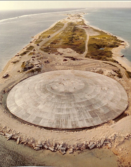
It is fitting that the Odums developed their approach at the start of what many consider to be the Anthropocene. The Odums viewed nature as a dynamic machine—an ecosystem—that operated autonomously but could also be adjusted, manipulated, and optimized by humans. It was a view of the natural world that gave humans a significant role. It is also fitting that they studied a South Pacific coral reef. Enewetak was one of the most isolated and wild places on the planet in the 1950s, but when the Odums arrived, it was already far from pristine. A couple years before, Enewetak had been the site of the first hydrogen bomb test. The explosion vaporized Elugelab, what had been one of Enewetak’s constituent islands. Successive tests followed, and the atoll became heavily contaminated with radioactive fallout. In the late 1970s, the United States attempted a half-hearted cleanup by scraping up the most easily reachable and lethal bits and entombing them in a massive concrete mausoleum (Fig. 3.1). The people of the Marshall Islands were treated no better. Many were forcibly displaced from their homes to make way for the nuclear tests, and nearly all have suffered the direct and indirect consequences of the subsequent contamination.5 Now human-induced climate change is threatening the ecological functioning of the reefs that support much of their well-being, and it is even threatening to submerge their island nation altogether.6
Coral reefs are just one of the many ecosystems whose functions, traits, and even existence are now under our uncertain stewardship. In this chapter, I explore how the Odum brothers’ ideas led to our current conceptualization of how the Earth System works. I then provide an extended definition of the ecosystem concept, focusing on the role that humans currently play in shaping nearly all of Earth’s ecosystems.
3.1 Follow the Energy
Section 3.1: Follow the Energy
The English plant ecologist Arthur Tansley coined the term “ecosystem” in a paper inauspiciously titled “The Use and Abuse of Vegetational Concepts and Terms.”7 A favorite pastime of plant ecologists at the time—and today—is to name notable associations of plants that make up the characteristic landscape of a region. These terms are handy when it comes to describing natural history. Field and natural history guides are filled with names that evoke the unique biology of a place: chaparral, deciduous forest, Douglas fir forest, shortgrass prairie. Tansley argued that focusing on just the organisms missed half the picture. Organisms interact with the physical environment around them, and for plants in particular, interactions with factors such as soil type and climate were just as important (if not more so) than the interactions among species. As Tansley (1935) put it:
But the more fundamental conception is, as it seems to me, the whole system (in the sense of physics), including not only the organism-complex, but also the whole complex of physical factors forming what we call the environment of the biome—the habitat factors in the widest sense [. . .] and there is constant interchange of the most various kinds within each system, not only between the organisms but between the organic and the inorganic. These ecosystems, as we may call them, are of the most various kinds and sizes.
Implicit in Tansley’s definition is the idea that interactions between organisms and between organisms and the physical environment create interchange pathways. But in his paper, Tansley never explicitly explained what is being exchanged or spent much time exploring how ecosystems might differ in the nature and magnitude of their interchange pathways.
After Tansley, ecologists started to fill in the picture, none more so than the two Odum brothers. The Odums defined Tansley’s vague interactions much more explicitly. They argued that the key feature of ecosystems is the flow of energy through them. The flow starts when photosynthesis captures solar radiation, storing it in the chemical bonds of sugar molecules. The captured energy powers all the physiological processes of life, and it gets passed along from organism to organism until every last bit of it has been used to do work, has been stored in more durable chemical forms, or has been converted back into radiation.
The Odum ecosystem model was more than a tweak to Tansley’s. It was a fundamentally different way of looking at the Earth System. Instead of individual species, it emphasized the processes that drive the flow of energy and the physical elements and molecules that flow along with the energy. This new perspective pushed the study of ecology in two important directions.
Describing Systems
Ecologists began to describe the natural world as complex dynamic systems. They were still interested in describing the distribution and abundance of organisms as well as how organisms interacted, but they also sought to describe the aggregate traits and characteristics of the systems as a whole. In many cases, the traits and metrics used to describe ecosystems were borrowed directly from the study of other complex systems such as economies and industrial processes. Ecologists started to describe life in terms that sounded more like a bank ledger than a natural history guide—things such as gross and net primary productivity and ecological efficiency. In their Enewetak study, the Odum brothers wrote up an energy balance sheet for the reef complete with a list of “income” and a list of “losses,” just as if they were auditing a surfside hamburger joint (Table 3.1). By the Odums’ accounting, most of the energy that was supporting the reef was generated on the reef itself, not imported from the much bigger ocean that surrounded it. Moreover, the reef had a balanced ledger. The energy that was fixed by photosynthesis on the reef plus the little bit that floated in as plankton from the surrounding ocean almost exactly matched the amount of energy used by reef organisms (expended as cellular respiration) or that flowed off the reef back out to the surrounding ocean. If anything, the reef ecosystem made a slight “profit” of energy that was stored in the persistent biomass and calcium carbonate shells of its organisms.
| Daily Energy Balance Sheet for Japtan coral reef Enewetak Atoll | |
|---|---|
| Energy inflow and outflow | Amount (g C/m2/day) |
| Income | |
| Plankton organic matter from the ocean | 2 |
| Photosynthesis on the reef | 24 |
| Subtotal | 26 |
| Losses | |
| Plankton organic matter lost to ocean | .4 |
| Total reef respiration | 24 |
| Subtotal | 24.4 |
| Net returns | 1.6 |
The common currency of energy allowed ecologists to summarize complex aggregations of life using a few key numbers that described how the aggregations generated and distributed energy. This allowed them to more easily compare and contrast ecosystems that were seemingly different in terms of their constituent parts. Some of the ecosystems that the Odum brothers applied their energy balance sheet to were the agroecosystems under development after the 1950s. Yield and overall agricultural output saw incredible improvements during the latter half of the twentieth century. But the Odums showed that our new agroecosystems had a different energy balance than coral reefs. The yield and output increases were not coming from energy fixed within the systems themselves. Instead, they were being driven by subsidized energy derived from fossil fuels. We were using energy that was biologically fixed in past ecosystems to produce our current food. The Odums worried that we were fooling ourselves into thinking that we had created an agro-industrial alchemy that would perpetually produce ever increasing yields, when in fact the energy balance sheet said that we were spending borrowed money. As Howard Odum (1971) put it, “This is a sad hoax, for industrial man no longer eats potatoes made from solar energy; now he eats potatoes partly made of oil.”
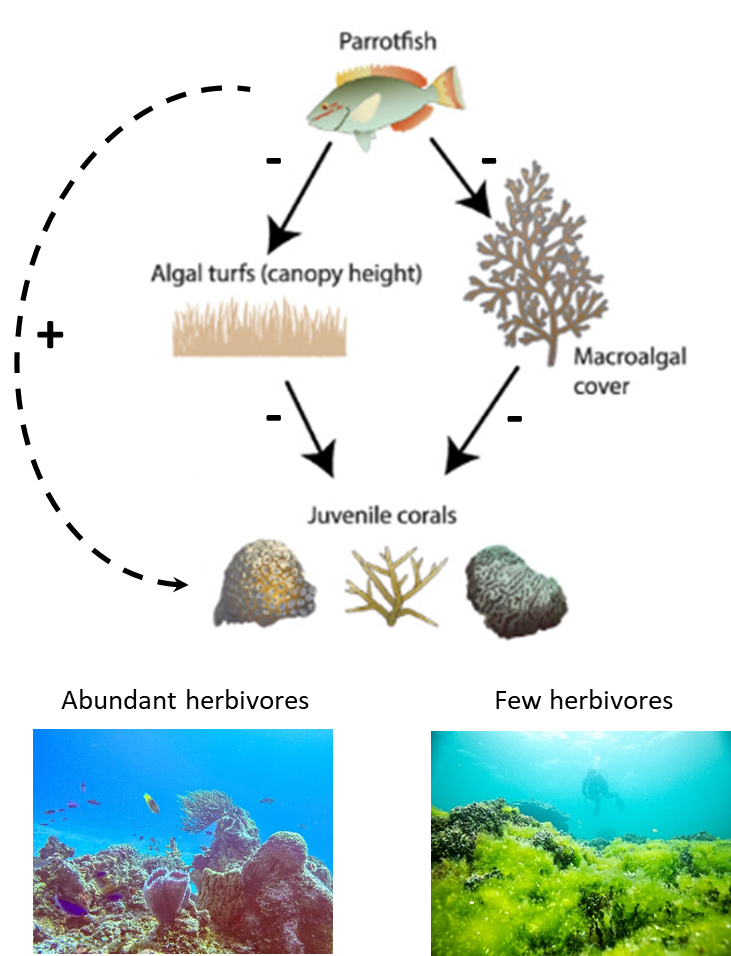
System descriptions also allowed ecologists to make more explicit predictions. They developed models that described how the component parts of ecosystems were linked into networks of interaction. They then used the models to predict what would happen if nodes were added or removed from the network, or if the strength of the interactions changed. Examples come from models of tropical coral reefs that added details to the original Odum model. From subsequent research, we know that while some of the photosynthesis on a reef is carried out by symbiotic algae living within coral polyps called zooxanthellae, a lot of it is also produced by free-living algae attached to the substrate.8 This is a bit surprising given the fact that we don’t usually see a lot of free-living algae on a tropical reef. This is because as soon as the algae can fix energy and convert it into biomass, a wide array of herbivorous fish eat it. As a result, much of the algae photosynthesis shows up in the form of abundant fish instead of thick carpets of algae. The fact that fish munch up a significant chunk of the reef’s energy gives them a large role in regulating where the energy goes and subsequently how the reef functions. With that information, researchers predicted that any changes to the abundance of herbivorous fish would have a big impact on coral reef characteristics (Fig. 3.2). Field studies have confirmed the prediction for many tropical reefs. Reefs where the abundance of herbivorous fish have been reduced because of factors such as overfishing often experience dramatic regime shifts from coral-dominant states to algae-dominant states.9
A Role for Humans
Before the Odum ecosystem concept, we tended to take a dispassionate outsider’s view toward describing nature. We classified its variation and described its interesting aspects like visitors to an art museum. Even when we used nature to provide benefits and services such as food, we tended to think of our use as incidental to the workings of nature itself. The Odum ecosystem concept allowed ecologists to easily plug humans into the system and to give them increasingly important roles. Humans could be parts of ecosystem machines just as easily as coral, algae, and fish could. If we could describe ecosystems as if they were a business, it was reasonable to think that we could manipulate the business in ways that maximized the benefits we got from it (e.g., food) or that minimized the harm we caused from our profit taking (e.g., overfishing). Just like an industrial engineer could optimize a manufacturing process, ecologists could examine the feedback and flow network of an ecosystem to identify components and steps that exerted the strongest influence on ecosystem traits that interested us, such as the abundance of fish. We could then make management recommendations that optimized our use of the system in various ways.
We also could start thinking about optimization in ways that went beyond the near-term direct benefits from ecosystems. We could attempt to optimize our use in ways that ensured the ongoing stability and sustainability of the system as a whole, or that prioritized nonhuman aspects of the system such as biodiversity. These concepts have informed many of the techniques and approaches that we currently use to help us better manage our interaction with the Earth System.
3.2 Ecosystems in the Anthropocene
Section 3.2: Ecosystems in the Anthropocene
All of Earth’s ecosystems can be described using the model in Figure 3.3. Granted, it is a big-picture view. There is no limit to the details it glosses over or leaves out altogether. For one, all the amazing biodiversity of the planet gets blithely labeled as the biotic environment. Still, the model succinctly describes the fundamentally unique way that our planet functions compared to the other planets in the solar system. The model has four main components.
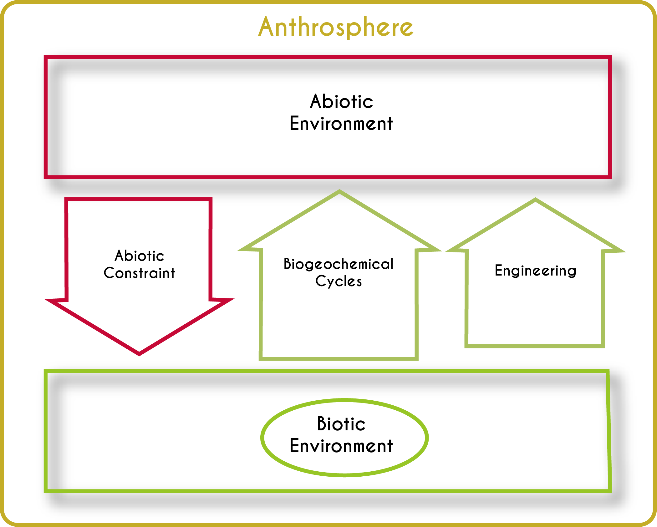
Abiotic-Biotic Feedbacks
Each planet has a characteristic set of nonliving parts and physical conditions. In Earth’s case, it has some typical rocks and minerals, a handful of atmospheric gasses, and a whole lot of liquid water. As far as we know, Earth stands out in one additional crucial respect: it has living organisms. Life inhabits nearly every centimeter of its surface as well as at least 3.8 km beneath its ocean floor,10 5 km below its continents,11 and 77 km up in its atmosphere.12 The abiotic and biotic parts of Earth interact, creating a web of interdependency. We can never really understand the abiotic parts of the world (things like the atmosphere and ocean) without understanding the ways in which organisms influence them, and we can never fully understand life without understanding how physical factors influence organisms. There are three main classes of these feedback (arrows in Fig. 3.3): abiotic constraints, biogeochemical cycles, and physical ecosystem engineering. I explore these feedbacks in more detail below.
Flows
The abiotic-biotic feedbacks drive the dynamic flow of energy and materials through ecosystems. This begins in most cases when photosynthetic organisms convert the electromagnetic energy transmitted by sunlight into chemical energy stored in carbohydrates. This energy then moves through ecosystems when organisms eat each other, parts of each other, or their wastes. The feeding (trophic) relationships among organisms create impossibly complex food webs. Although the flowing food forms intricate patterns, the flow of the energy embedded within the food tends to follow a stepwise progression from primary producers to herbivores to several successive levels of carnivores and sooner or later to detritivores (Fig. 3.4). Within each of these trophic levels, energy powers physical work, such as a redwood tree moving water from the soil to its leaves or a cheetah chasing a gazelle. The expenditure of energy to do work as well as the inherent inefficiency of metabolic processes means that only a small fraction of energy (on average about 10%) gets transferred from one trophic level to the next. That puts a fundamental constraint on how ecosystems look. There are always more individuals (and the packets of energy they reflect) in more basal trophic levels than in levels further down the energy supply line: more primary producers than herbivores, more herbivores than predators. All the energy that is captured by primary producers eventually either leaves Earth again as radiation (much of it as dissipated heat), or it gets put into long-term geologic (i.e., abiotic) storage such as in fossil fuels. Just as an engine needs a constant supply of fuel to keep running, the Earth System needs a constant supply of new energy from the sun to keep running.
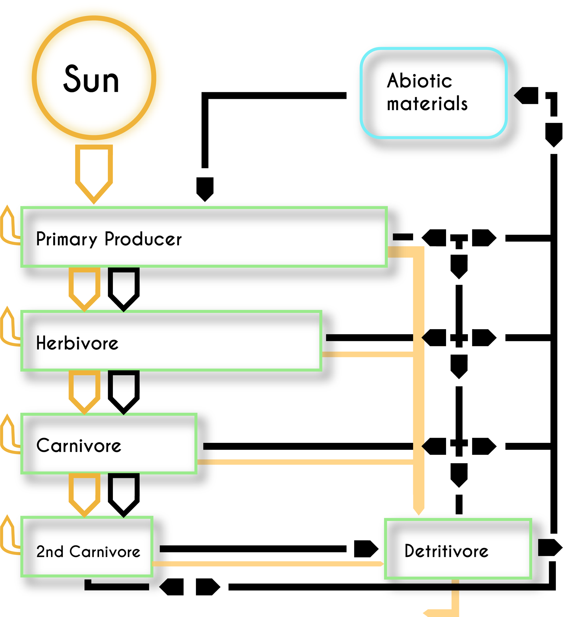
Much of the work that organisms use energy to do drives the spatial movement of physical things. This involves the direct movement of abiotic things, such as when plants transpire water from the soil to the atmosphere. It also involves the movement of organisms as well as the molecules and elements that flow through trophic pathways when organisms get eaten. In contrast to the flow of energy, the flow of elements and molecules form a more or less closed loop—ignoring the small fraction of the atmosphere that leaks into space and the occasional comet and asteroid impact that adds a few extraterrestrial bits. Materials get constantly recycled at both local and global scales.
Scale and Boundaries
The general model in Figure 3.3 doesn’t have a spatial scale; it can be applied to the entire Earth System as well as smaller parts of that system like my backyard. Spatial scale is an important aspect of ecosystems, however. All the processes and feedbacks that make up ecosystems have their own characteristic spatial scales. For instance, plants compete for water and soil nutrients within the spatial scale defined by their root systems, coral reefs attenuate wave energy across an area proportional to their size, and rivers distribute energy and materials across a terrestrial region defined by their watershed. Almost any ecosystem process you can think of has its own characteristic spatial scale that is in turn modified by the species involved and by a range of other idiosyncratic circumstances. That complexity makes it difficult to define innate spatial boundaries to ecosystems, although that hasn’t stopped us from trying. Perhaps the clearest boundary is between the entire biosphere and space. As we reduce the spatial scale of perspective, the appropriate boundaries get more difficult and subjective to delineate. We often use sharp disjunctions in biotic and abiotic conditions to delineate ecosystems, such as between the marine and terrestrial environments or between an alpine forest and a lowland desert. We also delineate spatial scales for more practical reasons. For instance, the Odums defined the scale of their study as a roughly 455 m × 2,000 m stretch of the Enewetak coral reef that they assumed to be representative of the entire reef. They likely chose that scale partly because of the limited time and money they had for their study. With more time and money, however, they could have defined things more broadly to encompass the entire atoll that includes terrestrial vegetation, the 80-km circumference lagoon, and the 40 small islands that dot the rim. There are many questions for which that larger scale is more appropriate. For example, to what degree does primary productivity from the reef subsidize the terrestrial communities on the atoll—or vice versa?
Ecosystem processes also have their own unique and varied temporal patterns. Timescale is therefore another important frame through which we can view and define ecosystem boundaries. The Odums conducted their study over six weeks during the summer. But the values of the ecosystem metrics they recorded undoubtedly fluctuate over the course of a seasonal cycle as well as from year to year. An annual or decadal energy budget might have a different bottom line than the few-week snapshot budget the Odums created.
One important result of all this spatial and temporal variability is that most ecologists no longer think of ecosystems as specific physical entities with clear, unambiguous boundaries like an individual organism has. Instead, ecosystems are more concepts than physical things. They are ways of describing interesting sets of ecological processes and interactions over interesting stretches of space and time. What those interesting stretches of space and time are is entirely a human decision.
Anthrosphere
As we saw in Chapter 1, the Earth System is increasingly influenced by human activities. We could lump these activates into the biotic environment box, but this would be too much of a simplification. Human activities are so pervasive and ubiquitous that the entire Earth System now operates within a human sphere of activity: the anthrosphere. This term is often used in a narrower way to describe obviously human-created habitats such as cities, and to distinguish those from less human-influenced habitats such as a coral reef. But human influence now goes way beyond our urban centers and touches almost every aspect of the Earth System. It is becoming difficult to describe ecosystems without recognizing (either explicitly or implicitly) human influence. The principal motivation for the Odums’ Enewetak study was to provide a baseline from which to assess the impact of nuclear testing on the reef system. Aboveground nuclear testing ended in 1963, but a range of other, perhaps more profound, human-driven perturbations have continued. Any study of the Enewetak reef today would need to acknowledge the context of rising sea surface temperatures, ocean acidification, nutrient pollution, and intensive fishing. Any baselines that are established today (on reefs or on any other part of the Earth System) are starting from a point that has already been significantly altered by human activities.
In the following sections, I explore the components of the Odum ecosystem model in more detail as well as the ways in which we now strongly influence each of the components.
3.3 All the World’s an Abiotic Stage
Section 3.3: All the World’s an Abiotic Stage
It is difficult to downplay the importance that the abiotic parts of the environment have on organisms. Nearly everything you can think of about the ecology of an organism is strongly influenced by the abiotic environment. In a sense, the abiotic environment is the stage upon which the play of life takes place—albeit a stage that is constantly rearranged by the players. This abiotic influence manifests itself in four main ways.
Physiology
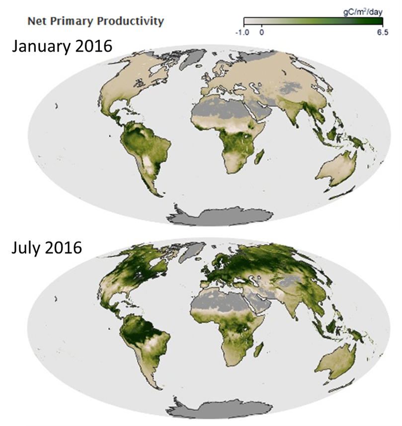
Abiotic conditions influence the rate of metabolic processes as well as the abundance and availability of the resources that organisms metabolize. Terrestrial plants are an excellent example. Plants are ectothermic, so the rate of photosynthesis varies with the ambient temperature. Plants also need water to conduct photosynthesis, so when it is in short supply, photosynthesis grinds to a halt. As a consequence, water and temperature are key regulators of how much photosynthesis happens in terrestrial ecosystems. If all you know is the rainfall and temperature of a region, you can make a fairly accurate prediction about how much photosynthesis is taking place there (Fig. 3.5).
Abundance and Geographic Range
All organisms require a specific set of environmental conditions in order to grow, reproduce, and survive. These conditions define an organism’s ecological niche. The degree to which conditions at any given spot or time meet the niche requirements for an organism determines whether the organism can live there, during what times, and in what abundance. Not all niche parameters are abiotic. Some involve interactions between organisms. For instance, the presence of a particularly strong competitor or predator, or conversely the absence of a necessary food item, can make local conditions unsuitable for an organism. Still, the abiotic components of niches tend to be more fundamental because before anything else, organisms first need to simply tolerate the local abiotic conditions. One indication of this importance is that changes in abiotic conditions often cause dramatic changes to the range or abundance of organisms.
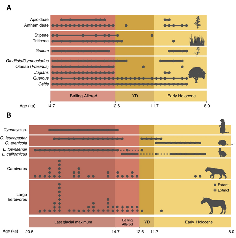
A good example comes from a trove of fossils deposited on the floor of Hall’s Cave in West Texas. The fossil deposits are something like a short historical film of the plants and animals that were living in the region at the end of the Pleistocene and start of the Holocene epochs about 20,000 to 8,000 years ago. This was a tumultuous period climatically, when the last great ice age was giving way to the warm period we have been experiencing ever since. The transition wasn’t smooth. About 47,000 years ago, global climate rapidly warmed during a period known as the Bølling–Allerød, immediately got colder again during the Younger Dryas (12,800 to 11,500 years ago), then steadily warmed into the Holocene. The fossils from Hall’s Cave show that the plants and animals living in the region also changed abruptly during this time.
During the last ice age, the region was a grassland that supported a large number and diversity of grazing animals such as bison and horses as well as burrowing ones such as prairie dogs. But as the climate warmed, the vegetation shifted to an open woodland, and the abundance of grazers and burrowing mammals declined (Fig. 3.6). As the Holocene progressed, many species that were functionally similar or closely related to the original inhabitants but that had environmental tolerances better suited to the new conditions colonized the area. Intriguingly, this wasn’t the case for the largest grazing animals and their predators, lending support to the hypothesis that hunting from newly arrived humans may have combined with climate change to cause the continent-wide extinctions of these large animals.13
Shorter-term climate and weather fluctuations also cause dramatic changes to the range and abundance of organisms. An example comes from the altered ocean conditions associated with El Niño-Southern Oscillation (ENSO). During the warm phase of ENSO, above-average sea surface temperatures prevail in the central and eastern tropical Pacific Ocean. As a result, warmwater tropical marine species such as mahi-mahi (Coryphaena hippurus) and striped marlin (Kajikia audax) often temporarily expand their range north into the temperate waters along the Pacific coast of North America. The warm and cool ENSO phases typically last about a year and recur every two to seven years or so, but on an irregular schedule. Other similar fluctuations have time spans on the order of decades. In the eastern Pacific, the abundance of anchovies and sardines fluctuate dramatically over periods of about 20 years. Anchovies thrive when relatively cool water conditions prevail, while sardines prefer it warmer. From the early 1950s to about 1975, the eastern Pacific was cooler than average, and anchovies dominated. Then, from about 1975 to the late 1990s, conditions warmed, and sardines dominated.14
Evolution and Form
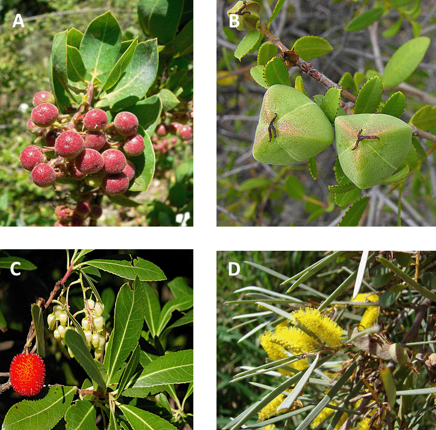
The abiotic environment is natural selection’s hammer. It is not the only selective force shaping the evolution of organisms, but it is brutal and unceasing. Nearly every aspect of an organism’s structure, form, physiology, and behavior partly reflects evolutionary adaptations to abiotic conditions. For instance, abiotic selective forces have driven many of the remarkable examples of convergent evolution, such as the morphological similarity between penguins and puffins and between cactuses and euphorbias. Perhaps because they are so constrained by place, plants seem to reflect their physical surroundings. For example, many of the woody plant species in the Mediterranean climate zone of Southern California have a morphology known as sclerophylly, characterized by having small, thick, hard, evergreen leaves that are often heavily protected with waxy cuticles or spines. The characteristic morphology reflects adaptations that help plants conserve water during the long, dry summers characteristic of the region. Plants in the other four Mediterranean climate regions have evolved remarkably similar adaptations (Fig. 3.7).
Our Influence on Abiotic Conditions
We profoundly alter Earth’s abiotic environment. Our cities are perhaps the clearest example. Nearly every aspect of the urban abiotic environment is either under our direct day-to-day management or is significantly influenced by our actions. The list includes temperature, humidity, wind, hydrology, light, and sound. I explore the urban environment in more detail in Chapter 8. Our influence over abiotic environments stretches far beyond cities. We now influence abiotic conditions everywhere on Earth, in a variety of ways, and across a range of scales. At a fundamental level, we do this by altering the two biological feedback mechanisms depicted in Figure 3.3: biogeochemistry and ecological engineering. I explore those mechanisms and our influence on them more explicitly in the following sections. Our manipulation of those two feedback mechanisms alters abiotic conditions in three general ways.
We Alter Resource Abundance and Availability
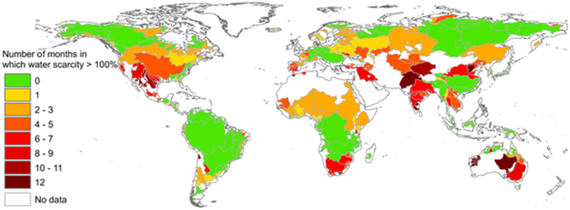
We use a lot of abiotic resources to feed ourselves, to construct our homes and workspaces, and to manufacture all the stuff we use in our daily lives. In the process, we move materials around the globe, altering their local abundance. The scale of our use and movement of resources has become immense. For example, globally, we now capture about 30% of all the annually available freshwater before it flows into oceans or it can recharge aquifers.15 We use some of that water like a library book: we briefly use it, then return it so that it is available for other uses. For example, most of the water involved in taking a quick shower flows back to the source we diverted it from—albeit a little dirtier than it started out. But we also consumptively use a lot of water in the sense that we make it unavailable to other organisms for long periods. This includes all the water that is incorporated into our bodies and those of our domesticated animals and crops, water that is transpired through crops or evaporates from fields, and much of the water used in manufacturing processes. Agriculture is by far our biggest consumptive use of water, making up 92% of our global water footprint.16 In many regions, our consumptive use of water frequently exceeds the amount of freshwater that is needed to support ecological functions, such as habitat for aquatic species, creating chronic water scarcity (Fig. 3.8).
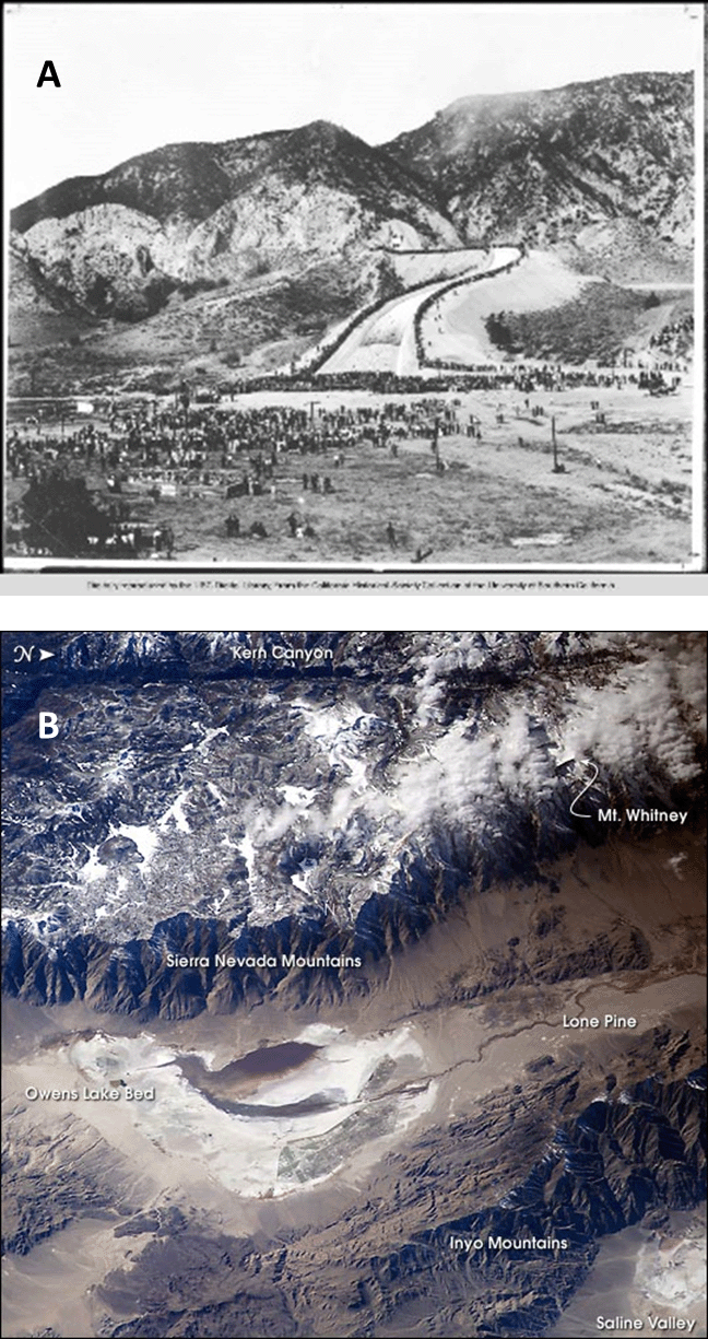
The process of supplying resources to human habitats can alter abiotic conditions in places far distant from where the resources are used. For example, in 1913, the city of Los Angeles, California, completed construction on an aqueduct to bring water into the city from the Owens River, located 375 km to the northeast. The movement of water turned what had been the 280 km2 Owens Lake into a dusty salt flat (Fig. 3.9). In addition to destroying an important aquatic habitat, the briny residue that was left turned into a dangerous fine particulate dust whenever the wind kicked up. For most of the past century, the Owens Dry Lake was the greatest single source of air pollution in the United States.17
The delivery mechanisms we use to move resources around are often inefficient, so that much of the resources leak away or otherwise don’t reach our intended target for them. This can create resource subsidies that alter physical conditions in places and at times that we did not intend. The flow of biologically reactive nitrogen is a great example. We apply large amounts of reactive nitrogen in the form of crop fertilizers, much of which is not taken up by crops. Globally, only about 47% of the reactive nitrogen applied to cropland is converted into harvested products.18 Much of the excess nitrogen enters waterways and alters nutrient levels at considerable distances from where the fertilizer was applied. For example, every summer, nutrient-laden runoff from farms and cities throughout the vast Mississippi River watershed fuels a boom of marine algae in the Gulf of Mexico that in turn causes a vast hypoxic dead zone to form.19
We Homogenize the Spatial and Temporal Variability of Conditions
When we create habitats for ourselves or our favorite species (such as our crops), we not only adjust the level of conditions but also alter the variability of conditions across space and time. We seem to have an innate compulsion to make abiotic conditions less variable than they otherwise naturally would be. We know what conditions we and our favored species like, and we attempt to keep things that way. While the temperature outside might be frigidly cold or swelteringly hot, the temperature inside our homes and workspaces tends to always be a bland 20°C. We have extended our homogenously benign conditions over large swaths of the planet. For example, much of the skill and art of agriculture involve devising ways to make conditions uniformly favorable for a relatively few crops. We use a variety of tools to help us do this, such as irrigation to even out the seasonal or yearly availability of water, tillage to make soil conditions more spatially uniform, and fertilizers to ensure a steady supply of nutrients.
As I describe in section 2.2, variable conditions help promote and maintain biodiversity. By extension, our tendency to reduce variability in conditions is a major way that we contribute to biodiversity loss. Our regulation of water by the use of dams is a good example. From our perspective, one of the key benefits of dams is that they smooth out annoying swings in water availability. Natural river flows tend to be seasonally episodic, with periods of high flow alternating with periods of low flow. There is also a lot of year-to-year variation in flow on top of that. By storing water behind dams, we can increase the availability of water during times it would otherwise be scarce or reduce its availability during times it would otherwise be superabundant. That’s good for our needs and goals, but it often disrupts the existing variability in water availability that other organisms depend on. Rivers have unique flow patterns that reflect their regional climate and the topography they flow through. For example, river basins in coastal forests of the US Pacific Northwest experience peak flows during the height of the rainy season in midwinter. Rivers farther east in the rain shadow of the Cascade Range receive much of their annual flow in the form of snowmelt, and consequently, their peak flows tend to happen in late spring and early summer. These regional differences in flow patterns have contributed to the United States having remarkably high levels of freshwater biodiversity. But the installation of dams along nearly all of the major river systems in the United States has significantly homogenized the timing and magnitude of river flows.20
We Alter Disturbance Patterns
Disturbance is a bit slippery to define, but in an ecological context, it usually means any temporary change to environmental conditions. These changes are typically acute, large in magnitude relative to baseline levels, and often cause the death of organisms or the removal of biomass
It is probably easier to give examples of disturbance than to precisely define it. A forest fire, a volcanic eruption, a flood, a hurricane, a gopher digging a burrow, a goat browsing on shrubs all cause temporary changes to abiotic and biotic conditions. Despite the often random and unpredictable nature of disturbances, ecosystems tend to have characteristic suites of disturbance types and typical patterns to the spatial distribution and timing of disturbances. For instance, hurricanes are a unique aspect of the climate along the US Gulf and Atlantic Coasts. Although the likelihood that a hurricane will affect a particular location in any given year is low, we know that it eventually will with a characteristic probability. We also know that hurricanes are most likely to form during the months from June to November (hurricane season). When hurricanes make landfall, they disrupt coastal ecosystems in a number of ways, including downing trees, inundating freshwater systems with salt water, and flooding areas with torrential rain. As a result, the physical structure and species composition at any location partly reflect its history of hurricane disturbance.21
Other regions and habitats have their own disturbance types as well as characteristic spatial and temporal patterns to those disturbances. That degree of consistency gives disturbance patterns the ability to shape the evolution and form of organisms. For instance, the sclerophyll life forms in Figure 3.7 partly reflect adaptations to the recurring late-summer and early-autumn fires that are characteristic of Mediterranean-type ecosystems. Fire is also a good illustration that disturbances strongly influence the abundance and flow of resources through ecosystems. In many ecosystems, fire releases nutrients that had been sequestered within the bodies of organisms such as long-lived trees, making them available for other organisms.22
We create our own unique types of disturbances, many of which are novel additions to ecosystems. These are often associated with the activities we do to extract resources (e.g., mining, harvesting a crop) or to construct our human environments (e.g., cutting a road through a forest, mowing a lawn, plowing a field). We also modify the existing pattern of disturbances in ecosystems. An important example of this is our modification of fire. Fire is one of the most widespread and important disturbances in terrestrial ecosystems. It shapes the life history of many organisms, it regulates the availability and flow of nutrients, and it is an important part of the global carbon cycle.23
We have been altering the pattern and intensity of fire on the planet for a long time, at least as far back as 1 million years ago.24 As mentioned in Chapter 1, early hunter-gatherers used fire as a tool to promote species they liked to eat, such as low-growing herbaceous plants and animals like deer. These species do well under the abiotic conditions that occur soon after a fire, such as high light and nutrient levels. In many parts of the world, we still use fire as a management tool, primarily as a way to clear land and provide good growing conditions for domesticated crops. In doing so, we often increase the fire frequency above the long-term historic baseline for an ecosystem. For example, until recently, fires had been rare across much of the Amazon basin. Any given patch of forest might have experienced a fire once every few hundred years, and in some places, the natural fire return frequency may be as long a thousand years.25 That pattern began to change starting around 1987, when both the number of fires and their frequency increased dramatically as new settlers colonized the region and used fire as a tool to clear forest.26 In other parts of the world, we have decreased the historical fire frequency by actively suppressing fire. This has been the case in many North American forests where fire suppression programs over the past 100 years have significantly reduced fire frequency. In many western forests, the longer fire return intervals have caused much more fuel in the form of living and dead plant biomass to accumulate between fire events. When a fire does manage to escape our vigilance, it is often larger and more intense (hotter for longer) than it has historically been.27
3.4 Biogeochemistry
Section 3.4: Biogeochemistry
Organisms suck molecules and elements out of the abiotic parts of the Earth System, chemically alter them in various ways, then release them back into the nonliving world. All that sucking and spewing intricately intertwines the workings of the biotic and abiotic parts of the Earth System. That amalgam of the living and nonliving is perhaps what is most unique and special about our planet. In a provocative paper titled “Atmospheric Homeostasis by and for the Biosphere: The Gaia Hypothesis,” atmospheric scientist Joseph Lovelock and microbiologist Lynn Margulis argued that life on the planet had collectively evolved to regulate the physical processes of the planet in ways that supported and enhanced life.28 They pointed out that life was not simply using the abiotic world; it was also actively manipulating abiotic conditions at the global scale. The provocative part of their argument was the idea that life had evolved to collectively manipulate the abiotic world in coordinated ways that supported life as whole.
As an example, they claimed it is not simply a random happy accident that the amount of CO2 sucked out of the atmosphere by photosynthesis nearly exactly matches the amount of CO2 that is spewed into the atmosphere by cellular respiration. They argued that the symmetry reflected an integrated system that had evolved to regulate atmospheric CO2 at levels that kept temperature and other abiotic conditions related to the carbon cycle within a range that was most conducive to life. Other biogeochemical cycles, they argued, similarly regulated Earth’s physical conditions within a just right sweet spot for life. The Lovelock and Margulis hypothesis was met with a lot of skepticism, mainly for the idea that life in aggregate had collectively evolved to coordinate their metabolic processes. A big conceptual hurdle is that natural selection largely works at the level of individuals. While the self-interest of individuals sometimes aligns with the broader good of life as a whole, it just as often does not. Efforts to come up with less teleological explanations for how self-stabilizing biophysical feedbacks could develop at the global scale have fallen short. While a few computer simulations have suggested that self-reinforcing and stabilizing biophysical feedbacks can potentially arise, not much empirical evidence has emerged to support the idea that natural selection has shaped their evolution or ongoing maintenance.29
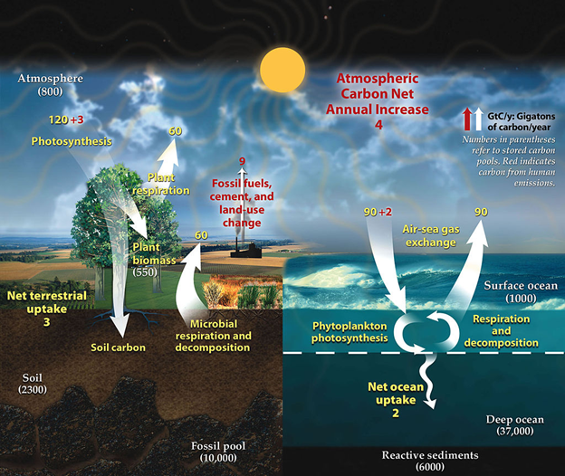
Although the evolutionary aspects of the Gaia hypothesis don’t have much support, its central theme, that life continuously transforms and shapes the basic characteristics of our planet, does have a lot of support. Through their biochemistry, organisms influence the dynamic flow of almost every element and molecule in the Earth System. In turn, almost all the traits we know and love about Earth—its temperature, how green it looks, how much fresh water it has available—partly reflect the biochemical alchemy of life. Lovelock and Margulis presented the flow of carbon as the archetypal example. At any given moment, Earth’s carbon is sitting in or flowing between five main reservoirs: the atmosphere, the bodies of living organisms and their dead parts, soil and sediment, the ocean, and the rocky crust (Fig. 3.10).
A substantial part of the flow between the five reservoir is driven by abiotic processes. For instance, atmospheric CO2 is constantly dissolving into and out of the ocean like a giant fizzy drink. But a substantial part is also driven by biochemical transformations, principally photosynthesis, respiration, and methanogenesis. As Lovelock and Margulis pointed out, that biologically driven flow has a large influence on global climate because it helps determine the concentration of carbon-containing greenhouses gases (mainly CO2 and CH4) in the atmosphere. I explore the carbon cycle and its influence on global climate in more detail in Chapter 4. Climate is just one abiotic trait that the levels of carbon-containing compounds affect. Other notable conditions include the pH of the oceans and the availability of soil nutrients used by plants.
Biochemical transformations are mostly carried out by the tiniest forms of life: microorganisms. Despite the primary role that they play in shaping our world, we probably know the least about microorganisms than any other group of life. That’s partly because they are invisible to the naked eye, are difficult to study in the wild, and even harder to study in captivity. Even when we can directly observe and study them, they often don’t seem very exciting, at least at first glance. The have just a handful of prosaic morphological types that, judging by names such as gram-negative and gram-positive, even microbiologists don’t find that exciting. But whatever microbes lack in terms of morphological majesty, they more than make up for in their metabolic prowess.
There is hardly an element or molecule that isn’t metabolized by one microbe or another. At least one strain of soil bacteria is even capable of digesting polyurethane plastic and, if necessary, use the plastic to supply all its energy, carbon, and nitrogen.30 The importance of microbes also stems from the fact that they are everywhere. The primary limiting constraint to life on Earth seems to be the availability of liquid water, even if only in intermittently tiny amounts. Microbes are found everywhere that basic constraint is met. That includes thriving in habitats that seem extreme to us, such as scalding thermal vents or blocks of ice.31
The lives of microorganisms are also intricately intertwined with those of all other life. Many of the biochemical functions carried out by multicellular organisms are performed or mediated by symbiotic relationships with microorganisms.32 For instance, the ability of terrestrial plants to efficiently extract nutrients and water from the soil is largely dependent on their symbiotic relationships with mycorrhizal fungi.33 Even the chloroplast and mitochondria organelles that drive photosynthesis and respiration in multicellular organisms were once free-living microbes.34
Our Influence on Biogeochemical Flows
When the Gaia hypothesis was first formulated in the 1970s, it was part of a growing scientific appreciation for the ways in which life influences the Earth System. That growing appreciation of the transformative power of life included our own activities. In the subsequent years, we have gained a much more detailed understanding of the direct and indirect ways in which we alter biogeochemical flows.
Direct Alteration to Flows
One of the principal ways that we influence biogeochemical flows is by carrying out our own chemical reactions, often on a massive scale. The outputs of those chemical processes can augment existing flows of elements and molecules. Our combustion of fossil fuels that adds to the flow of carbon from mineral forms in the crust to the atmosphere is a prime example (Fig. 3.10). Another example is our creation of biologically reactive nitrogen compounds. The world has a lot of nitrogen, but most of it is in biologically inert forms such as the nitrogen gas (N2) that makes up 78% of our atmosphere. Organisms can only use nitrogen when it is in more biologically reactive compounds such as ammonia (NH3) and nitrogen dioxide (NO2).
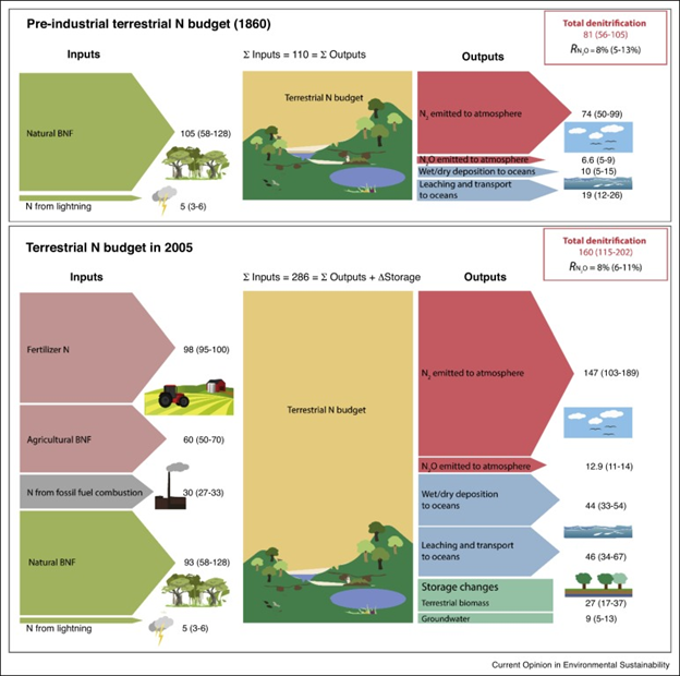
Until recently, the only sources of these reactive forms had been a few groups of bacteria that have the remarkable biochemical ability to create them from atmospheric N2, plus a smidgeon more that is created when lightning forms nitric oxide (NO) from N2. That changed in 1910 when Fritz Haber and Carl Bosch succeeded in pulling off a biochemical feat of their own. The Haber-Bosch process suddenly allowed us to create reactive nitrogen in the form of prodigious amounts of NH3. We also produce reactive nitrogen as a by-product of fossil fuel combustion, and when we plant domesticated crops such as clover that have symbiotic relationships with nitrogen-producing microorganisms. All together, we now generate about half of the reactive nitrogen that is circulating through the planet at any given time. Put another way, we have roughly doubled the size of Earth’s reactive nitrogen flow since the nineteenth century (Fig. 3.11).
In addition to developing industrial reactions that mimic those carried out by microorganisms, we have created entirely new chemical formulations. Novel materials are one of the hallmarks of the Anthropocene. Not surprisingly, most of these new or previously rare materials aren’t used by organisms for food or to support their physiological processes. Aluminum is a good example. Although aluminum is the third most abundant element in the Earth’s crust, no known organism needs it to live, and it doesn’t seem to play a role in any essential biological process.35 The fact that life evolved to largely ignore aluminum may be related to the fact that most of it is bound up in biologically inaccessible mineral compounds.36 Elemental aluminum used to be extremely rare in the Earth System before we developed ways to industrially produce it in the late 1800s. Aluminum is now a ubiquitous component of our modern life; since 1950, we have added about 500 Tg of elemental aluminum to the Earth System.37 Although organisms don’t use aluminum, it is far from biologically inert. Partly because it is now much more commonly encountered by organisms, we are beginning to document a wide range of ways aluminum influences biological systems, many of them negative. For instance, aluminum is acutely toxic to many organisms, particularly under acidic conditions.38
Many other new or newly abundant materials do get biochemically transformed by organisms (usually by microbes), or they enter food webs. An example are the industrial pollutants known as polychlorinated biphenyls (PCBs). While most organisms don’t readily metabolize PCBs, PCBs do bind tightly to lipids. As a result, they can progressively build up in the bodies of organisms (bioaccumulate), becoming increasingly concentrated in the tissues of organisms as they move up through trophic levels.39 Even though their use has declined in recent years, PCBs are now ubiquitous parts of ecosystems. They have even been found in the tissues of amphipods living in ocean trenches more than 10,000 m deep.40
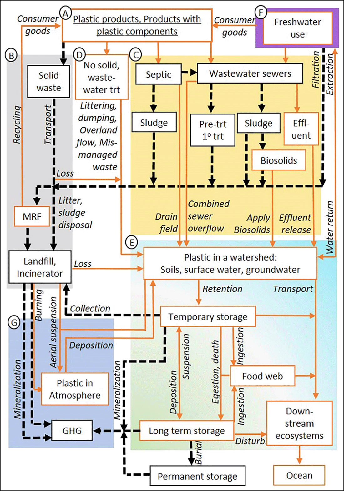
The movement and transformation of our manufactured materials through the Earth System create entirely new biogeochemical flows. An important characteristic of these new flows is the outsized role that we play in them. The plastic cycle is a good example (Fig. 3.12). We chemically manufacture plastics from other materials, regulate their release to various ecosystems, and chemically transform them back into their constituent materials.
Indirect Alteration to Flows
We also alter biogeochemical flows in indirect ways. One of these is by changing the environmental conditions for other organisms. Because many important biochemical transformations are carried out by relatively few types of microorganisms, altering conditions for just a few species can often have a large impact on cycles. For example, a key property of soil is how much organic matter it contains. Organic matter influences a range of other soil properties such as water and nutrient availability, which in turn influence the vegetation the soil can support. Soil organic matter consists primarily of plant and animal parts in various stages of decay, and its abundance in soil is largely a balance between photosynthesis that creates biomass and decomposition that transforms it back into its constituent parts. Key players in that balance are the soil microbes that use soil organic matter as a food source. In doing so, they convert carbon that had been fixed into carbohydrates via photosynthesis back into CO2 through respiration. In many terrestrial ecosystems, the flow of carbon into the soil from photosynthesis to form soil organic carbon is a bit greater than the flow of carbon out of the soil from microbial respiration. As a result, soils in many places tend to accumulate large stores of carbon over time. In some habitats like tidal wetlands, whose waterlogged anaerobic sediments inhibit microbial respiration, the balance is even more decidedly lopsided toward carbon storage.41 Globally, soils have an average net carbon uptake of 3 gigatonnes (Gt) per year, and the total amount of carbon in soil is almost three times the amount in the atmosphere (Fig. 3.10). Our activities have significantly altered that balance sheet.
The biggest impact has come from the conversion of ecosystems into intensive forms of agriculture. The details vary a lot depending on the region and ecosystems involved, but in many instances, agricultural soils tend to have abiotic conditions that are more favorable for decomposing microorganisms than the conditions in the nonagricultural soils they replaced. For instance, draining and tilling wetland soils create the more oxygenated conditions required by aerobic bacteria that are big contributors to decomposition. An example comes from the Sacramento–San Joaquin River Delta at the back of San Francisco Bay. Beginning in the nineteenth century, a network of levees was constructed throughout the delta, and the land behind the levees was drained and converted to agriculture.
The drained lands promoted a burst of microbial respiration that is actively converting stored soil organic matter into greenhouse gasses. Drained sites release up to 341 g C m−2 yr−1 of CO2 and 11.4 g C m−2 yr−1 of CH4. The peat soils behind the levees have vanished into thin air. The delta is now dotted with inverted islands that are as much as 4.6 m (15 ft) below sea level.42 In contrast, delta sites that have been restored back to wetlands sequester up to 397 g C m−2 yr−1. The restored wetlands do emit more CH4 than agricultural sites because methane-producing bacteria (methanogens) thrive in the anaerobic conditions, but this is compensated for by the significant reduction in soil respiration.43 The conversion of wetlands to agriculture is an extreme example, but similar changes happen when most other habitat types are converted to agriculture. Globally, habitat conversion to agriculture has resulted in the loss of 133 petagrams (Pg) of C from the soil;44 a petagram is 1012 kg.
Another factor contributing to the greater carbon sequestration of wetlands compared to farms is the fact that much more of the carbon fixed by photosynthesis in the wetlands flows into their waterlogged soils. On farms, much of the crop biomass gets harvested and fed into pathways (like our mouths) that more readily produce greenhouse gasses. Our appropriation of materials is another way that we influence environmental conditions for organisms, which in turn can further alter biogeochemical flows. While appropriation implies a taking away, it also involves augmentation. As I describe above, one of the main ways that we alter abiotic conditions in ecosystems is by spatially rearranging materials such as water. We divert the flow of materials away from some locations and organisms and augment the flow to other locations and organisms. Those changes can in turn influence the local physical and biotic drivers of biogeochemical flows.
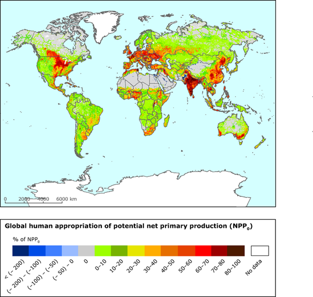
The case of the water diversion from Owens Lake is an example. The diversion significantly reduced primary production in Owens Lake, while the steady subsidy of water to the urban landscapes and outlying farms of Los Angeles increased primary production there. We increasingly divert materials on massive scales. Averaged across the planet’s terrestrial ecosystems, we appropriate about 25% of Earth’s potential terrestrial net primary production (NPP) by harvesting crops, by causing land use changes that affect productivity (such as replacing forests with a cities), and by setting fires.45 In some regions, we appropriate the vast majority of the potential net primary production (Fig. 3.13).
Our creation, appropriation, and movement of materials creates unique spatial patterns of flow that are influenced more by economic efficiencies and trade patterns than by ecological relationships. In a sense, we now act like competing chemical engineers who have rearranged the pipes and valves that make up Earth’s biochemical factory. Natural gas extracted from Texas can be used to make ammonia in a Louisiana chemical plant that is then used to fertilize a Brazilian maize field whose grain is then eaten by an Argentinean cow whose flesh is then eaten by an Arsenal Football Club supporter in a London pub. That one thread of global trade directly and indirectly drives the spatial flow of hundreds of elements and innumerable molecules. The flows alter environmental conditions across scales from the amount of soil carbon on a Brazilian farm, to nitrogen levels in the Thames estuary, to the global concentration of atmospheric CO2.
3.5 Ecosystem Engineering
Section 3.5: Ecosystem Engineering
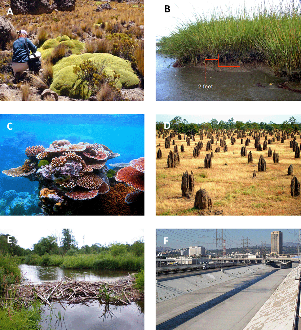
Biochemical transformations are not the only way that organisms modify the planet. They also construct things at a more macroscopic scale. Every organism builds a body: tiny ones like the silica-based cell walls of diatoms, delicate ones like a western pygmy blue butterfly, or massively grand ones like a giant sequoia. Many organisms also actively build structures separate from their own bodies. Examples are tunnels created by moles, dams created by beavers (Fig. 3.14E), and architecturally avant-garde termite mounds (Fig. 3.14D). Both types of structure modify the physical environment by altering the flow of energy or materials. Tree canopies block sunlight and attenuate wind energy. The stems of salt marsh plants slow down flowing water, trapping sediment and attenuating wave energy. Soil-crust-forming microorganisms bind soil particles together into impervious pavement that blocks and channels the flow of rainwater. Beaver dams block the flow of stream water, creating deep, still ponds. The excavations of earthworms create air spaces in soil, increasing its permeability to water. These types of interactions are collectively called physical ecosystem engineering. While every organism engages in ecosystem engineering, some organisms are particularly good at it (Fig. 3.14).
At first glance, the distinction between biochemical transformation and ecosystem engineering may seem a bit arcane. Both involve organisms that modify the flow or state of matter and energy. But there are a few ecologically interesting distinctions. When organisms biochemically modify elements and compounds, the transformation is closely linked to the physiology of the organism. Factors that affect the rate of those physiological processes also affect the rate of biochemical transformation, and when the organism dies, the transformations immediately stop altogether.
In engineering, the modifying structures often have a measure of autonomy from the organisms that build them. For example, beavers actively maintain dams for several years (sometimes up to a decade), but eventually they abandon the dam when the adjacent local food resources become depleted. The abandoned dams continue to alter environmental conditions long after the beavers are gone. The dams do slowly decay without constant maintenance, but the decay rate depends on local environmental conditions, not the activities of the long-gone beavers.46 Structures can also outlive organisms even when the structure is the body of the organism itself. For instance, when trees die, they often remain upright for years as forest snags. As the snags slowly decay, they provide habitat for a complex succession of organisms such as cavity nesting birds.47
Unlike the case with biochemistry, the degree of habitat modification caused by ecosystem engineering may not directly correspond to the current local abundance or activity of organisms. Structures (and the habitat modifications they influence) can accumulate in the landscape as the individuals that made them come and go. The calcium carbonate exoskeletons produced by mollusks and reef-building coral are great examples. Fossilized reefs created by shell-building organism that lived 500 million years ago are still actively modifying the physical environment for benthic organism living along the shore of Chesapeake Bay today.48
Although the ability of structures to outlive the organisms that made them is an important aspect of ecosystem engineering, the active maintenance of structures is also an important attribute. The habitat produced by ecosystem engineering is constantly being made—and remade—by organisms themselves. At times, this can look like the cooperative environmental regulation outlined in the Gaia hypotheses.
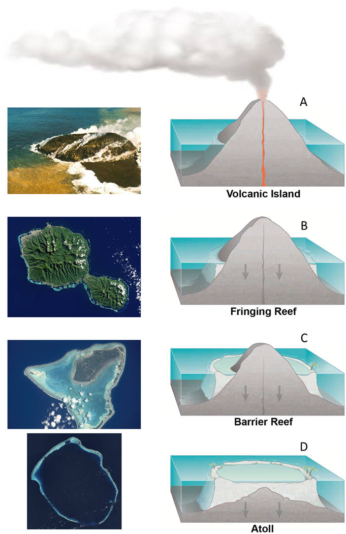
The algae symbionts of coral can only live in shallow water where there is enough light for photosynthesis. On reefs that form coral atolls such as Enewetak, the ideal depth range is partly maintained by the reef itself. Atoll reefs originally start out as fringing reefs that encircle volcanic islands. When the source of magma feeding the island volcano stops, the crust supporting the island slowly deflates like a balloon with a leak in it. The island and its fringing reef then begin to sink back under the waves. If conditions are favorable for coral growth and the rate of island submergence isn’t too fast, however, than the coral can keep pace. Every year, the coral adds a layer of calcium carbonate to an ever taller circular tower of coral skeletons. The growing tower keeps the algae in the sunny shallows, which keeps the coral and its supporting tower growing. Eventually, the only thing visible above the ocean surface is a circular reef surrounding a shallow lagoon (Fig. 3.15).
The structures created by ecosystem engineering often alter suites of abiotic conditions to a much greater extent than individual biochemical processes do. These suites of changes effectively create entirely new abiotic habitats that can influence whole communities of organisms. Perhaps even more so than biogeochemistry, ecosystem engineering creates the complex biophysical landscape that is the habitat of all life. Coral reefs (Fig. 3.14C) are classic examples of this kind of habitat construction. A few of the important coral modifications include attenuating tidal and wave energy, providing hard attachment points for sessile organisms such as sponges, and creating a complex three-dimensional structure for more active organisms like fish. The constructed habitat of coral reefs supports some of the most diverse and complex assemblages of biodiversity on the planet. All together, coral reef habitats support roughly 32% of all the named multicellular marine species on Earth.49
The physical activities of organisms also create habitats. Charles Darwin documented a great example. Soon after returning home from his around-the-world trip, Charles Darwin turned his attention to the activities of the earthworms in the garden of his country home. Darwin saw that earthworms physically reworked the soil as they fed. They dragged seeds, leaves, and other bits of organic matter from the surface down to deeper soil layers and in return brought deeper soil up to the surface. Darwin estimated that earthworms in his garden moved 17 to 40 tonnes of soil to the surface each year. Most of that soil had been physically altered by the worms as it passed their digestive system. These worm castings made up the majority of the topsoil at his house and across the surrounding English countryside.50 Many of the physical changes caused by earthworms are directly beneficial to plants. These include masticating organic matter into tiny bits, facilitating its decomposition into plant useable nutrients, increasing soil aeration, and promoting water infiltration. At a global scale, the presence of earthworms is estimated to increase crop yields by 25%.51 As Darwin (1892) put at the end of his book about earthworms:
The plough is one of the most ancient and valuable of man’s inventions; but long before he existed the land was in fact regularly ploughed, and still continues to be thus ploughed by earthworms. It may be doubted whether there are many other animals which have played so important a part in the history of the world, as have these lowly organized creatures.
Even relatively static plants can do a surprising amount of earth-shaping physical work. The bodies of terrestrial plants act as physical pumps that move liquid water from the soil into their roots, up through their shoots, and out through their stomata as water vapor. Most of the energy to move the water is passively derived from solar energy heating leaf surfaces as well as the molecular cohesion of water molecules. But plants actively regulate every step of the process, most significantly by opening and closing their leaf stomata. Globally, terrestrial plants move an estimated 62,000 ± 8,000 km3 of water per year from the soil to the atmosphere, accounting for 80% to 90% of all the water moving from the soil to the atmosphere. All that pumping uses half of all the solar energy absorbed by Earth’s land surfaces.52
Human Alteration of Ecosystem Engineering
Humans have become some of the most accomplished ecosystem engineers on the planet. We also indirectly alter engineering processes by altering the abundance, distribution, and behavior of other organisms that are themselves strong ecosystem engineers.
Human Constructions
We create a diversity of durable and long-lived structures using materials appropriated from the Earth System. These include things like buildings, bridges, and walls that we typically think of as structures as well as some less obvious things such as plastic bottles and telephone poles. These structures are among the most obvious signatures of the Anthropocene. The total mass of all our human-made material is now something more than 1.1 teratonnes, that’s greater than all living biomass on Earth. To put that in a bit more context, the weight of all the plastic we have added to the world (8 Gt) is twice the weight of all the animals on Earth. All the buildings, roads, and other human infrastructure in the world weighs about 1,100 Gt, while all its trees and shrubs only weigh about 900 Gt.53
Our structures modify the flow of energy and materials through the environment in ways that are often analogous to the structures created by other organisms. For instance, both beaver- and human-constructed dams divert water and influence local hydrology in broadly similar ways. But our accelerating technological and industrial ability is allowing us to build structures at spatial scales that exceed the capabilities of many of the most industrious and abundant nonhuman engineers. A comparison with beavers provides an illustration. North American beaver (Castor canadensis) were introduced to the main island of Tierra del Fuego in 1946. Since then, the beavers (and their dams) have spread throughout the Tierra del Fuego archipelago, dramatically altering the hydrology and landscape of the region. On the main island, beaver densities can exceed 15 dams per km2.54 One study estimated that on the Argentinian half of the island, beavers had modified 31,000 ha, about 1.6 % of the total area.55 In contrast, at the northern end of Argentina, along the border with Paraguay, just one human-constructed dam, the Yacyretá Dam, forms a 110,000-ha lake out of the Paraná River. Five hundred kilometers upstream, the Itaipu Dam forms a 135,00-ha lake.56
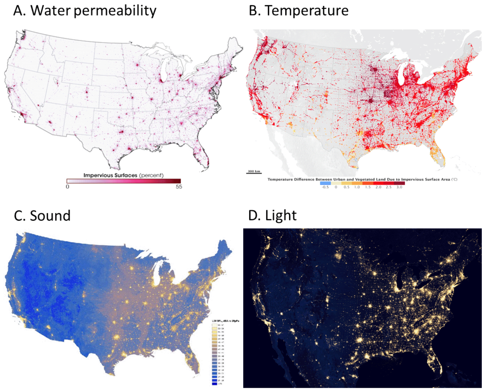
We stitch together our human structures into an extensive network of urban areas, industrial facilities, roads, walls, aqueducts, and communication lines. The physical properties of this built network in turn modify myriad abiotic conditions. For instance, common building materials such as asphalt and concrete are generally a bit better at absorbing solar radiation than vegetated landscapes. In addition, much of the solar energy that vegetation does absorb goes to powering transpiration instead of generating heat. In contrast, hardscapes spend the day absorbing shortwave solar radiation, then releasing it back out as long wave radiation (heat). As a result, landscapes that have a lot of constructed materials tend to be warmer than ones with a lot of vegetation. Averaged over the year, a modest-sized city of 1 million people is about 1°C to 3°C warmer than the surrounding landscape.57 Figure 3.16 depicts the built structure network of the United States in terms of four important environmental factors that it influences: the flow of rainwater, local ambient temperature, sound, and nighttime light. Urbanized environments tend to produce higher volumes of polluted rainwater runoff and are warmer, nosier, and brighter at night than the surrounding landscape. I describe urban environments in more detail in Chapter 8.
Just like many nonhuman ecosystem engineers, humans also dynamically modify existing physical structure. One of the more significant examples is soil tillage. Tillage alters many of the physical properties of soil. Among others, these changes include making soil more finely textured, friable, aerated, warmer, and less capable of holding water than untilled soil of the same type.58 We currently periodically till a bit less than 11% of Earth’s habitable land.59 In some regions, the proportional area being tilled is much greater. For instance, nearly half of India’s land area is tilled at least occasionally.60 I describe how tillage affects the soil environment in a bit more detail in Chapter 7.
Indirect Influence on Ecosystem Engineering
In addition to creating and modifying our own structures, we indirectly affect ecosystem engineering by altering the abundance of nonhuman ecosystem engineers. We do this by making environmental conditions more or less favorable for them and by introducing them to regions outside of their native range. A good example comes from smooth cordgrass (Spartina alterniflora; Fig. 3.14B). Smooth cordgrass is native to the East and Gulf Coasts of North America where it forms the structural foundation of salt marsh habitat. Its dense stems and roots trap sediment, raising the relative elevation of the surrounding marsh. Elevation is a key environmental attribute in the marginal borderland between land and sea. Even seemingly small changes in elevation can radically alter abiotic conditions such as salinity and oxygen levels in the sediment. The dense cordgrass canopy also greatly reduces the amount of sunlight reaching the sediment, which in turn influences factors such as temperature and salinity. The stems provide physical attachment points for sessile organisms as well as protective cover for organisms hiding from predators.61 In all, the physical habitat created by smooth cordgrass supports a diverse community of organisms, including many species that we harvest for food.62 In addition, the wave-absorbing properties of smooth cordgrass also provide important storm protection.63
Despite this importance, we have been contributing to the decline of smooth cordgrass across much of its native range. The decline is a result of many interacting factors, including nutrient pollution, oil spills, cutting erosion promoting channels, and altering the supply of sediment to the marsh.64 That last factor is particularly important. In much the same way that atoll-building coral maintain their relative elevation with respect to sea level, cordgrass can maintain the relative elevation of marshes even as sea level rises by trapping sediment and growing a prodigious underground root system. But we have disrupted this process by channeling rivers and diverting sediment away from marsh distributaries. Without sediment to trap and with less cordgrass to trap it even if it was there, marshes have been washing away. In Louisiana, 4,900 km2 of coastal wetlands—about 16% of the original marsh area—have turned into open water over the past 80 years.65
In an odd twist, we have been causing the opposite process along many temperate Pacific coastlines. Salt marshes in the temperate Pacific are notably distinct from those in the temperate Atlantic by historically not having large Spartina species such as smooth cordgrass. Pacific coastal wetlands tend to be dominated by open mudflats instead of densely vegetated salt marshes. We have dramatically changed things by introducing smooth cordgrass and several other Spartina species. Their establishment and spread have engineered a complete transformation of mudflat habitats into dense cordgrass meadows in many regions. The physical changes associated with this introduction have in turn altered the entire ecology of estuaries from the amount of habitat available for juvenile fish, to the type of invertebrate species inhabiting the mud, to the abundance of food and nest sites available to birds.66
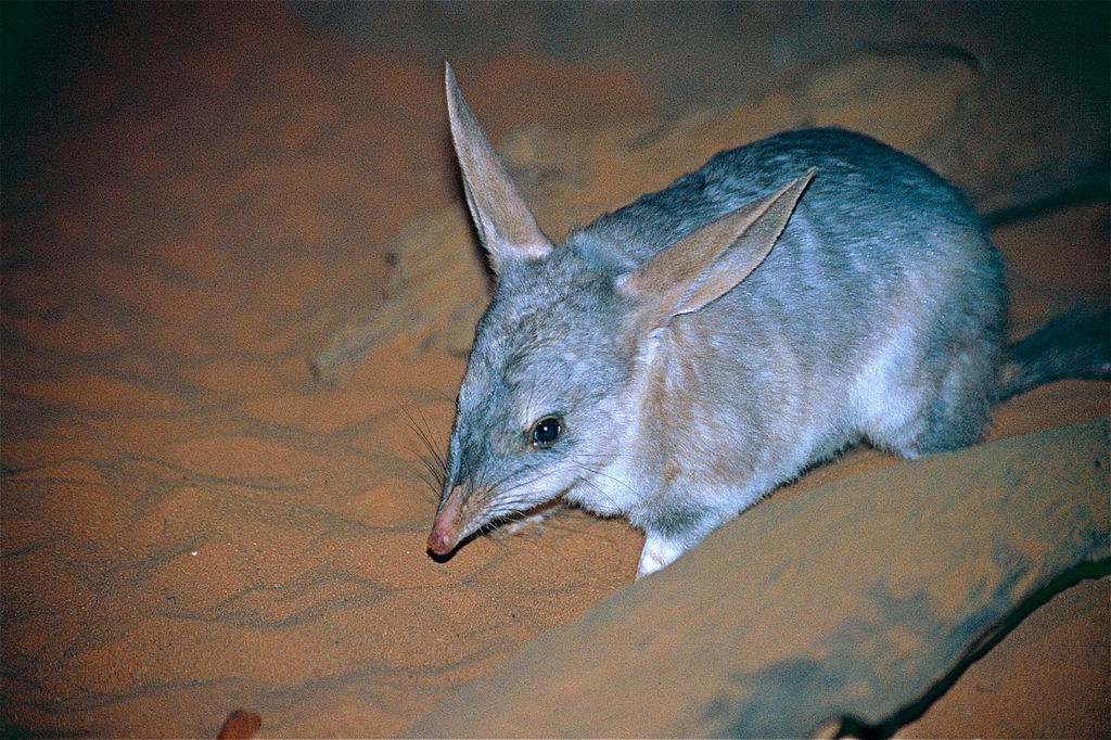
We also change the abundance of strong animal ecosystem engineers. The North American beavers introduced to Tierra del Fuego (mentioned above) are an example. Another example comes from Australia. Australia is (or was) home to several species of native digging mammals such as bilbies (Fig. 3.17) and bettongs (Bettongia spp.). These little digging mammals have had a big effect on the soils of Australia. As they forage for food, they create small soil pits that collect organic matter and water, sort of like how the nooks and crannies of a couch collect loose change and old French fries. The little creatures are industrious as well as cute. At one site in southwestern Australia, each individual woylie (Bettongia penicillata) turns over 4.8 tonnes of soil per year.67 Yet we have caused the dramatic decline of Australia’s digging animals, mostly by introducing non-native predators that are particularly adept at eating them such as red foxes (Vulpes vulpes) and feral cats (Felis catus). They are now extremely rare or absent altogether from large swaths of the continent. Among the only places that they attain their former abundance are within fenced predator-free reserves. The abundant diggers have significantly modified soils within the reserves.
Soils in predator-free reserves have higher organic material and available carbon, nitrogen, phosphorus, and water-holding capacity than soils in adjacent areas. These changes are particularly significant in the nutrient-poor and dry soils that exist across much of Australia.68 When eastern bettong (Bettongia gaimardi) were reintroduced to a predator-free reserve in southeastern Australia, their digging created germination sites that preferentially favored native grassland species over the numerous non-native species that were also at the site. That little bit of help from the bettongs as well as some management help from us could allow the native plants to persist in the landscape even in the face of competition from non-native plants.69
3.6 The Ghost in the Machine
Section 3.6: The Ghost in the Machine
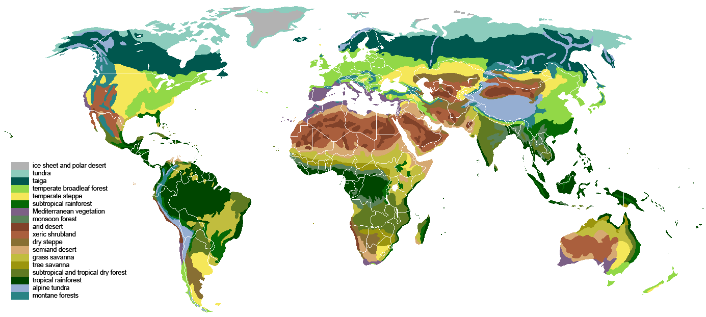
Our increasing influence over how the Earth System looks and functions is forcing us to revise how we describe and classify it. You probably have seen a map of the world’s terrestrial biomes (Fig. 3.18). The biome concept is an extension of Arthur Tansley’s ecosystem definition, where both organisms and the abiotic world interact to form unique and identifiable associations. For example, the extreme cold and aridity of arctic regions promote a treeless landscape of dwarf shrubs, grasses, and lichen known as tundra, while at the other end of the spectrum, the warm and wet conditions in some parts of the tropics support lush tropical forests. At smaller spatial scales, other details such as soil type, fire frequency, local microclimate, and the degree of geographic isolation foster characteristic spatial associations of organism and environmental conditions.
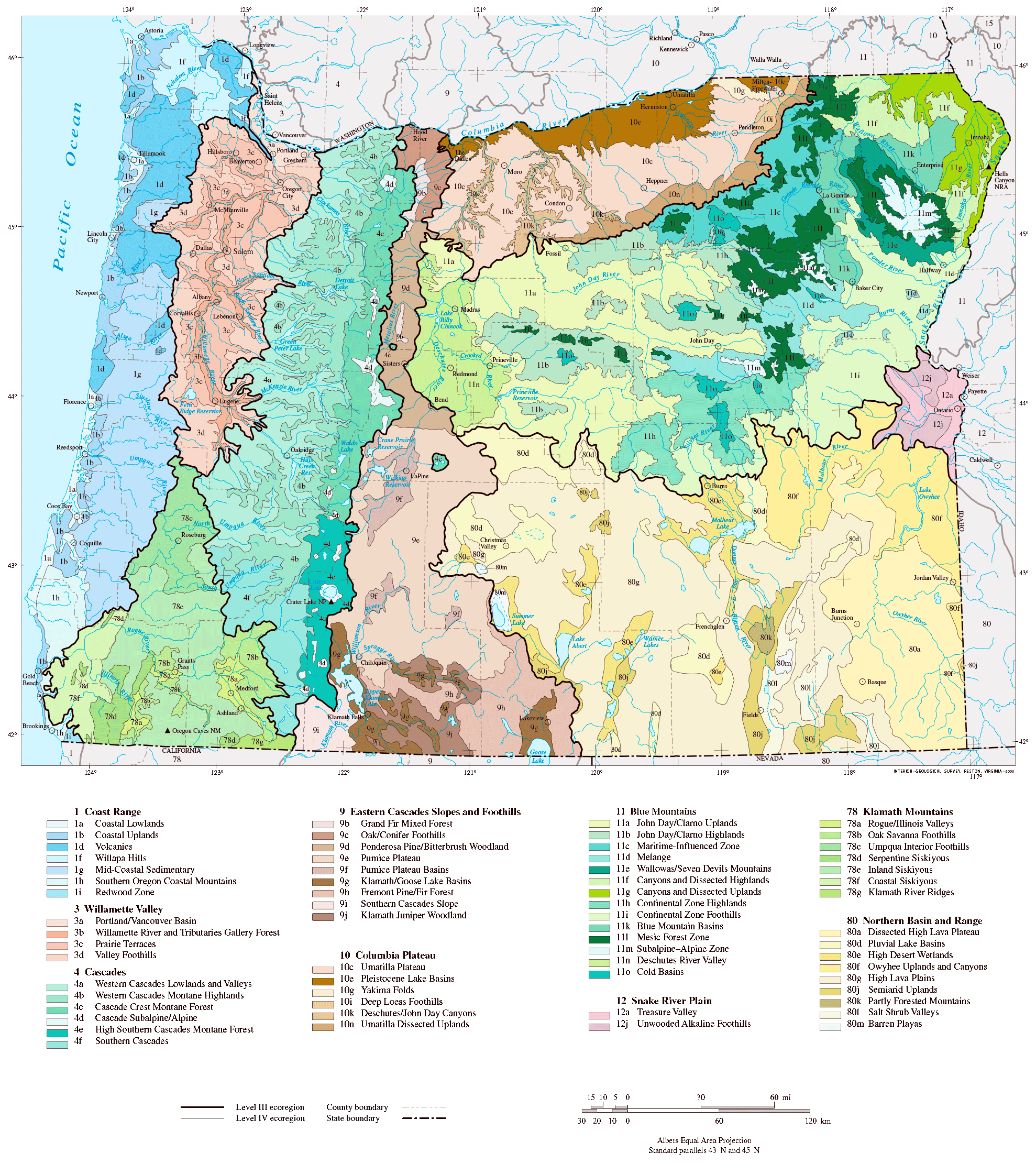
Ecoregions are a classification system for describing these hallmark associations. The US Environmental Protection Agency uses a system of four spatially nested categories. The coarsest Level I scale classifies the continental United States into 12 ecoregions, while the finest Level IV scale classifies it into 967 ecoregions. Figure 3.19 is a map of the Level III and IV ecoregions in the state of Oregon. Ecoregions and other similar classification are a concise way of summarizing the natural history of a region. Ecoregion maps describe in shorthand the biological diversity of regions and how that diversity varies across landscapes. For example, the map of the Level III and IV ecoregions in Oregon illustrates how ecosystem-level diversity increases as you move from west to east across the state (Fig. 3.19). Ecoregions are also useful tools for helping to manage our use of natural resource. Classification systems similar to ecoregions are used to identify suitable areas for growing different crops, to predict irrigation requirements, and to identify appropriate plant choices for ornamental landscapes in urban areas.
Despite how useful these classification systems are, many of them have an important drawback in the age of the Anthropocene: they downplay our own influence. When we first developed them, we understandably based them on natural abiotic and biotic conditions. We mostly wanted to describe the natural world, not the parts of it that we had redesigned. As this chapter has outlined, however, the parts of the world that we have redesigned have grown dramatically. We now exert a strong influence on ecosystems over wide stretches of the planet. Ecologists began to realize that biomes as well as the more detailed ecoregion classifications should do a better job of reflecting the human-altered landscapes that increasingly cover the planet. For example, I live in Corvallis, Oregon, whose EPA Level III ecoregion is called Willamette Valley Prairie Terraces. Here is its official description:
The nearly level to undulating Prairie Terraces ecoregion includes all of the terraces of the Willamette River upstream of the Portland/Vancouver Basin (3a). Ecoregion 3c is drained by low-gradient, meandering streams and rivers. Its broad fluvial terraces once supported oak savanna and prairies that were maintained by burning; wetter areas supported Oregon ash and black cottonwood. Today, only relict native prairie remain. The poorly drained soils derived from glacio-lacustrine deposits are extensively farmed for grass seed and small grains. Grasses tolerate poor drainage and poor rooting conditions better than other crops. In addition to agriculture, the Prairie Terraces also experience the bulk of urban expansion.70
It describes the ecoregion as a primarily human construction. Even the namesake prairie (mentioned in the past tense) was itself a human construction, designed and maintained by Indigenous peoples before the arrival of Europeans.71
Other classification systems describe our influence even more explicitly. In 2008, Erle Ellis and Navin Ramankutty published a map of the world’s anthropogenic biomes, known as anthromes.72 The anthrome map emphasizes how the intensity and type of human influence vary across the planet. The current anthrome classification system has 19 terrestrial biome types, only 2 of which are classified as wildlands. In this system, wildlands are defined as areas that do not have human settlements or agriculture. The other 17 anthromes span the wide range of different ways we use ecosystems as well as the different intensities of that use. These include dense urban settlements, agricultural landscapes of various types, and sparsely populated but subtly manipulated rangelands and forests (Fig. 3.20). Looked at this way, more than 75% of the Earth’s ice-free land has been directly modified by humans to some extent. Just 22% of the land surface is wild.73 In some parts of the world, such as most of Europe and large chunks of North America, nearly the entire landscape has been modified by humans. A travel game I like to play is to look for parts of the landscape that we have not directly constructed or modified in some way. In many places, that is harder to do than you might at first appreciate.
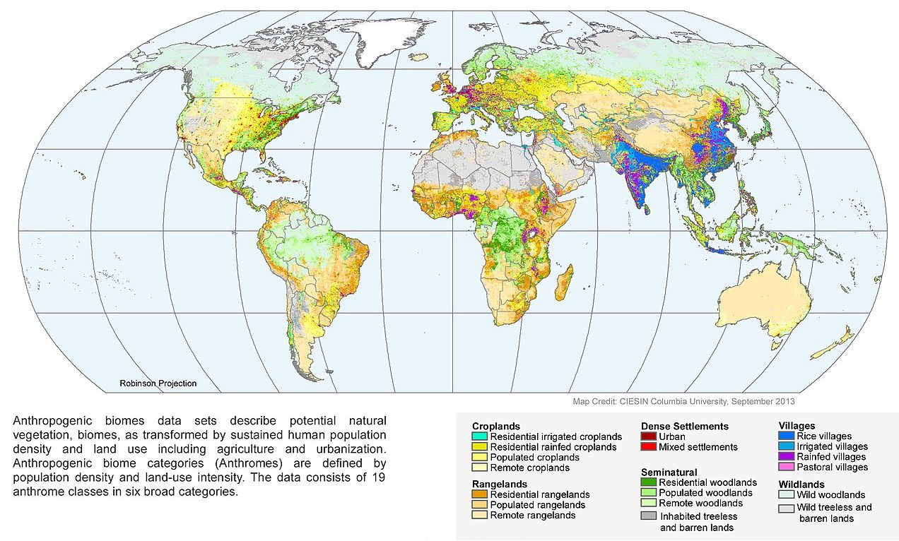
We can classify the ocean in a similar way, although we need to adjust our classification a bit. Hardly anyone lives on the ocean (although there are a few floating communities), so much of it could be considered wilderness if we use Ellis and Ramankutty’s terrestrial definition of wildland. But we intensively use and alter conditions across large stretches of ocean through activities such as intensively fishing, causing nutrient pollution, creating disruptive lights and sound, introducing non-native species, and using the ocean as a waste dump (Fig. 3.21). One way to define ocean wildness is to identify areas that experience human impact intensities in the bottom 10% of the observed range in global values. Using that measure, just 13% of the world ocean is still wild.74
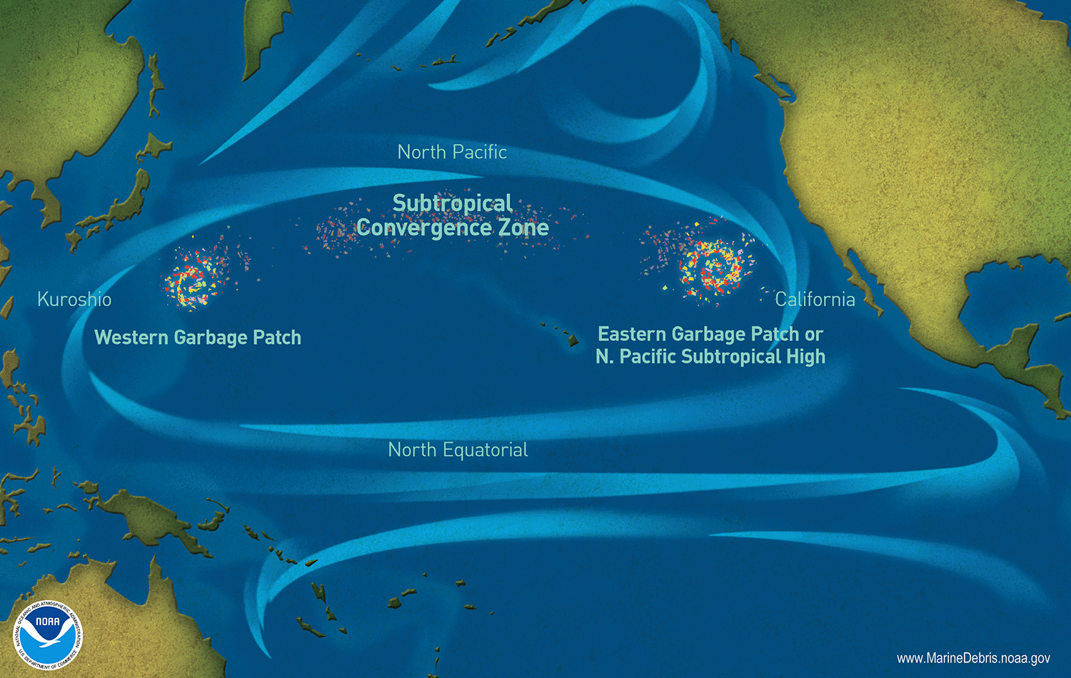
Even in the few wild places left on the planet, such as remote tropical forests and polar oceans, our influence is far from zero. Our activities have insinuated themselves into nearly every part of the global Earth System. We have become the ghost in the machine, at once just one part of the intricate Earth System but also increasingly its principal conductor, orchestrating the pace, timing, and intensity of its fundamental processes.
Chapter Summary
Anthrome Planet
The ecosystem concept is a way of conceptualizing and describing the Earth System in terms of how solar energy flows through its abiotic and biotic components. Humans are now the dominant force shaping energy and material flows on the planet. We do this in a number of direct and indirect ways to such an extent that we have insinuated our influence into almost every aspect of the Earth System.
- The Earth System is made up of living and non-living components that dynamically interact with each other (Figure 3.3)
- The physical environment sets fundamental constraints on key organism processes such as photosynthesis (Figure 3.5) and directs natural selection (Figure 3.7)
- In turn, organisms shape the physical environment through their biochemical processes (Figure 3.10) and the physical structures they create (Figure 3.14)
- Organisms also interact with each other by competing, facilitating, and eating. These interactions—particularly the eating—direct the flow of energy and materials through the Earth System (Figure 3.4)
- Humans now significantly influence each of those main nodes of interaction.
- We alter the abiotic environment by altering the abundance and availability of resources (Figures 3.8, 3.9), homogenizing physical conditions across space and time, and altering disturbance patterns
- We alter biological feedbacks on the physical environment through our own biochemistry (Figures 3.10, 3.11, 3.12), by altering or appropriating the biochemistry of other organisms (Figure 3.13), by creating physical structures (Figure 3.16), and by altering the distribution and abundance of structures created by other organisms (Figure 3.17)
- Our influence now extends across the Earth. Less than 22% of the Earth’s ice-free land is still wild and largely free of human influence (Figure 3.20)
Additional Resources
- Read about how the United States eventually cleaned up Enewetak Atoll after nuclear testing stopped, and how the island is now threatened by the potentially even more devastating specter of climate change: A Pacific Isle, Radioactive and Forgotten.
- Listen to a story about the burning season in Brazil’s Amazon region: In The Amazon’s Fire Season, ‘You Either Burn Or You Starve’.
References
15Albert, J.S., Destouni, G., Duke-Sylvester, S.M., Magurran, A.E., Oberdorff, T., Reis, R.E., Winemiller, K.O., Ripple, W.J., 2021. Scientists’ warning to humanity on the freshwater biodiversity crisis. Ambio 50, 85–94. https://doi.org/10.1007/s13280-020-01318-8
11Barras, C., 2021. Deepest land microbes ever found. New Sci. 249, 14. https://doi.org/10.1016/S0262-4079(21)00308-0
39Beyer, A., Biziuk, M., 2009. Environmental fate and global distribution of polychlorinated biphenyls. Rev. Environ. Contam. Toxicol. 201, 137–58. https://doi.org/10.1007/978-1-4419-0032-6_5
23Bowman, D.M.J.S., Balch, J.K., Artaxo, P., Bond, W.J., Carlson, J.M., Cochrane, M.A., D’Antonio, C.M., DeFries, R.S., Doyle, J.C., Harrison, S.P., Johnston, F.H., Keeley, J.E., Krawchuk, M.A., Kull, C.A., Marston, J.B., Moritz, M.A., Prentice, I.C., Roos, C.I., Scott, A.C., Swetnam, T.W., Werf, G.R. van der, Pyne, S.J., 2009. Fire in the Earth System. Science 324, 481–84. https://doi.org/10.1126/science.1163886
14Chavez, F.P., Ryan, J., Lluch-Cota, S.E., C, M.Ñ., 2003. From anchovies to sardines and back: multidecadal change in the Pacific Ocean. Science 299, 217–21. https://doi.org/10.1126/science.1075880
24Crutzen, P.J., Andreae, M.O., 2016. Biomass burning in the tropics: impact on atmospheric chemistry and biogeochemical cycles. In: Crutzen, P.J., Brauch, H.G. (Eds.), Paul J. Crutzen: A Pioneer on Atmospheric Chemistry and Climate Change in the Anthropocene. SpringerBriefs on Pioneers in Science and Practice. Cham, Switzerland: Springer, 165–88. https://doi.org/10.1007/978-3-319-27460-7_7
*Darwin, C., 1892. The Formation of Vegetable Mould through the Action of Worms: With Observations on Their Habits. J. Murray , London.
12DasSarma, P., Antunes, A., Simões, M.F., DasSarma, S., 2020. Earth’s stratosphere and microbial life. Curr. Issues Mol. Biol. 38, 197–244. https://doi.org/10.21775/cimb.038.197
68Decker, O., 2020. Losing Australia’s native gardeners. Science 370, 925. https://doi.org/10.1126/science.abf1706
2DeLoughrey, E.M., 2013. The myth of isolates: ecosystem ecologies in the nuclear Pacific. Cult. Geogr. 20, 167–84. https://doi.org/10.1177/1474474012463664
22Doerr, S.H., Cerdà, A., 2005. Fire effects on soil system functioning: new insights and future challenges. Int. J. Wildland Fire 14, 339–42. https://doi.org/10.1071/WF05094
53Elhacham, E., Ben-Uri, L., Grozovski, J., Bar-On, Y.M., Milo, R., 2020. Global human-made mass exceeds all living biomass. Nature 588, 442–44. https://doi.org/10.1038/s41586-020-3010-5
73Ellis, E.C., Ramankutty, N., 2008. Putting people in the map: anthropogenic biomes of the world. Front. Ecol. Environ. 6, 439–47. https://doi.org/10.1890/070062
57Environmental Protection Agency, 2008. Reducing Urban Heat Islands: Compendium of Strategies. Washington, DC: Environmental Protection Agency.
30Espinosa, M.J.C., Blanco, A.C., Schmidgall, T., Atanasoff-Kardjalieff, A.K., Kappelmeyer, U., Tischler, D., Pieper, D.H., Heipieper, H.J., Eberlein, C., 2020. Toward biorecycling: isolation of a soil bacterium that grows on a polyurethane oligomer and monomer. Front. Microbiol. 11. https://doi.org/10.3389/fmicb.2020.00404
3536Exley, C., 2009. Darwin, natural selection and the biological essentiality of aluminium and silicon. Trends Biochem. Sci. 34, 589–93. https://doi.org/10.1016/j.tibs.2009.07.006
35Exley, C., 2013. Aluminum in biological systems. In: Kretsinger, R.H., Uversky, V.N., Permyakov, E.A. (Eds.), Encyclopedia of Metalloproteins. New York: Springer, 33–34. https://doi.org/10.1007/978-1-4614-1533-6_105
*Field, M.E., Cochran, S.A., Evans, K.R., 2002. U.S. Coral Reefs—Imperiled National Treasures. USGS Fact Sheet 084-01. Santa Cruz, CA: US Geological Survey.
49Fisher, R., O’Leary, R.A., Low-Choy, S., Mengersen, K., Knowlton, N., Brainard, R.E., Caley, M.J., 2015. Species richness on coral reefs and the pursuit of convergent global estimates. Curr. Biol. 25, 500–505. https://doi.org/10.1016/j.cub.2014.12.022
67Garkaklis, M.J., Bradley, J.S., Wooller, R.D., 2004. Digging and soil turnover by a mycophagous marsupial. J. Arid Environ. 56, 569–78. https://doi.org/10.1016/S0140-1963(03)00061-2
6Giardino, A., Nederhoff, K., Vousdoukas, M., 2018. Coastal hazard risk assessment for small islands: assessing the impact of climate change and disaster reduction measures on Ebeye (Marshall Islands). Reg. Environ. Change 18, 2237–48. https://doi.org/10.1007/s10113-018-1353-3
5Goldsmith, C., 2014. Bombs over Bikini: The World’s First Nuclear Disaster. Minneapolis, MN: Twenty-First Century Books .
61Gutiérrez, J.L., Jones, C.G., Byers, J.E., Arkema, K.K., Berkenbusch, K., Commito, J.A., Duarte, C.M., Hacker, S.D., Lambrinos, J.G., Hendriks, I.E., Hogarth, P.J., Palomo, M.G., Wild, C., 2011. Physical ecosystem engineers and the functioning of estuaries and coasts. In: Wolanski, E., McLusky, D. (Eds.), Treatise on Estuarine and Coastal Science. Waltham, MA: Academic Press, 53–81. https://doi.org/10.1016/B978-0-12-374711-2.00705-1
45Haberl, H., Erb, K.-H., Krausmann, F., 2014. Human appropriation of net primary production: patterns, trends, and planetary boundaries. Annu. Rev. 39: 363-91.
8Hatcher, B.G., 1990. Coral reef primary productivity: a hierarchy of pattern and process. Trends Ecol. Evol. 5, 149–55. https://doi.org/10.1016/0169-5347(90)90221-X
55Henn, J.J., Anderson, C.B., Martínez Pastur, G., 2016. Landscape-level impact and habitat factors associated with invasive beaver distribution in Tierra del Fuego. Biol. Invasions 18, 1679–88. https://doi.org/10.1007/s10530-016-1110-9
54Herrera, A.H., Lencinas, M.V., Manríquez, M.T., Miller, J.A., Pastur, G.M., 2020. Mapping the status of the North American beaver invasion in the Tierra del Fuego archipelago. PLoS One 15, e0232057. https://doi.org/10.1371/journal.pone.0232057
56Herschy, R.W., 2012. World Lake Database: International Lake Environment Committee Foundation (ILEC). In: Bengtsson, L., Herschy, R.W., Fairbridge, R.W. (Eds.), Encyclopedia of Lakes and Reservoirs. Dordrecht, Netherlands: Springer, 920–21. https://doi.org/10.1007/978-1-4020-4410-6_188
16Hoekstra, A.Y., Mekonnen, M.M., 2012. The water footprint of humanity. Proc. Natl. Acad. Sci. 109, 3232–37. https://doi.org/10.1073/pnas.1109936109
*Hoekstra, A.Y., Mekonnen, M.M., Chapagain, A.K., Mathews, R.E., Richter, B.D., 2012. Global monthly water scarcity: blue water footprints versus blue water availability. PLoS One 7, e32688. https://doi.org/10.1371/journal.pone.0032688
*Hoellein, T.J., Rochman, C.M., 2021. The “plastic cycle”: a watershed-scale model of plastic pools and fluxes. Front. Ecol. Environ. 19, 176–83. https://doi.org/10.1002/fee.2294
9Hughes, T.P., Rodrigues, M.J., Bellwood, D.R., Ceccarelli, D., Hoegh-Guldberg, O., McCook, L., Moltschaniwskyj, N., Pratchett, M.S., Steneck, R.S., Willis, B., 2007. Phase shifts, herbivory, and the resilience of coral reefs to climate change. Curr. Biol. 17, 360–65. https://doi.org/10.1016/j.cub.2006.12.049
10Inagaki, F., Hinrichs, K.-U., Kubo, Y., Bowles, M.W., Heuer, V.B., Hong, W.-L., Hoshino, T., Ijiri, A., Imachi, H., Ito, M., Kaneko, M., Lever, M.A., Lin, Y.-S., Methé, B.A., Morita, S., Morono, Y., Tanikawa, W., Bihan, M., Bowden, S.A., Elvert, M., Glombitza, C., Gross, D., Harrington, G.J., Hori, T., Li, K., Limmer, D., Liu, C.-H., Murayama, M., Ohkouchi, N., Ono, S., Park, Y.-S., Phillips, S.C., Prieto-Mollar, X., Purkey, M., Riedinger, N., Sanada, Y., Sauvage, J., Snyder, G., Susilawati, R., Takano, Y., Tasumi, E., Terada, T., Tomaru, H., Trembath-Reichert, E., Wang, D.T., Yamada, Y., 2015. Exploring deep microbial life in coal-bearing sediment down to ~2.5 km below the ocean floor. Science 349, 420–24. https://doi.org/10.1126/science.aaa6882
42Ingebritsen, S.E., Ikehara, M.E., Galloway, D.L., Jones, D.R., 2000. Delta Subsidence in California: The Sinking Heart of the State. Fact Sheet 005-00. Reston, VA: US Geological Survey.
40Jamieson, A.J., Malkocs, T., Piertney, S.B., Fujii, T., Zhang, Z., 2017. Bioaccumulation of persistent organic pollutants in the deepest ocean fauna. Nat. Ecol. Evol. 1, 0051. https://doi.org/10.1038/s41559-016-0051
52Jasechko, S., Sharp, Z.D., Gibson, J.J., Birks, S.J., Yi, Y., Fawcett, P.J., 2013. Terrestrial water fluxes dominated by transpiration. Nature 496, 347–50. https://doi.org/10.1038/nature11983
74Jones, K.R., Klein, C.J., Halpern, B.S., Venter, O., Grantham, H., Kuempel, C.D., Shumway, N., Friedlander, A.M., Possingham, H.P., Watson, J.E.M., 2018. The location and protection status of Earth’s diminishing marine wilderness. Curr. Biol. 28, 2506-12. https://doi.org/10.1016/j.cub.2018.06.010
64Kennish, M.J., 2001. Coastal salt marsh systems in the U.S.: a review of anthropogenic impacts. J. Coastal Res. 17, 731-48.
48Kidwell, S.M., 1986. Taphonomic feedback in Miocene assemblages: testing the role of dead hardparts in benthic communities. PALAIOS 1, 239–55. https://doi.org/10.2307/3514688
29Kirchner, J.W., 2002. The Gaia hypothesis: fact, theory, and wishful thinking. Clim. Change 52, 391–408. https://doi.org/10.1023/A:1014237331082
43Knox, S.H., Sturtevant, C., Matthes, J.H., Koteen, L., Verfaillie, J., Baldocchi, D., 2015. Agricultural peatland restoration: effects of land-use change on greenhouse gas (CO2 and CH4) fluxes in the Sacramento-San Joaquin Delta. Global Change Biol. 21, 750–65. https://doi.org/10.1111/gcb.12745
58Lal, R., 1991. Tillage and agricultural sustainability. In: Lal, R. (Ed.), Soil Tillage for Agricultural Sustainability, special issue, Soil Tillage Res. 20, 133–46. https://doi.org/10.1016/0167-1987(91)90036-W
18Lassaletta, L., Billen, G., Grizzetti, B., Anglade, J., Garnier, J., 2014. 50 year trends in nitrogen use efficiency of world cropping systems: the relationship between yield and nitrogen input to cropland. Environ. Res. Lett. 9, 105011. https://doi.org/10.1088/1748-9326/9/10/105011
28Lovelock, J.E., Margulis, L., 1974. Atmospheric homeostasis by and for the biosphere: the Gaia hypothesis. Tellus 26, 2–10. https://doi.org/10.1111/j.2153-3490.1974.tb01946.x
47Lutz, J.A., Larson, A.J., Swanson, M.E., Freund, J.A., 2012. Ecological importance of large-diameter trees in a temperate mixed-conifer forest. PLoS One 7, e36131. https://doi.org/10.1371/journal.pone.0036131
3Martin, L.J., 2018. Proving grounds: ecological fieldwork in the Pacific and the materialization of ecosystems. Environ. Hist. 23, 567–92. https://doi.org/10.1093/envhis/emy007
31Merino, N., Aronson, H.S., Bojanova, D.P., Feyhl-Buska, J., Wong, M.L., Zhang, S., Giovannelli, D., 2019. Living at the extremes: extremophiles and the limits of life in a planetary context. Front. Microbiol. 10, 780. https://doi.org/10.3389/fmicb.2019.00780
62Minello, T., Webb, J., 1997. Use of natural and created Spartina alterniflora salt marshes by fishery species and other aquatic fauna in Galveston Bay, Texas, USA. Mar. Ecol. Prog. Ser. 151, 165–79. https://doi.org/10.3354/meps151165
17National Academies of Sciences, 2020. Effectiveness and Impacts of Dust Control Measures for Owens Lake. Washington, DC: National Academies Press. https://doi.org/10.17226/25658
4*Odum, H.T., 1971. Environment, Power, and Society. New York: Wiley-Interscience.
*Odum, H.T., Odum, E.P., 1955. Trophic structure and productivity of a windward coral reef community on Eniwetok Atoll. Ecol. Monogr. 25, 291–320. https://doi.org/10.2307/1943285
65Olea, R.A., Coleman, J.L., 2013. A synoptic examination of causes of land loss in southern Louisiana as related to the exploitation of subsurface geologic resources. J. Coastal Res. 1025–44. https://doi.org/10.2112/JCOASTRES-D-13-00046.1
41Ouyang, X., Lee, S.Y., 2020. Improved estimates on global carbon stock and carbon pools in tidal wetlands. Nat. Commun. 11, 317. https://doi.org/10.1038/s41467-019-14120-2
20Poff, N.L., Olden, J.D., Merritt, D.M., Pepin, D.M., 2007. Homogenization of regional river dynamics by dams and global biodiversity implications. Proc. Natl. Acad. Sci. 104, 5732–37. https://doi.org/10.1073/pnas.0609812104
19Rabalais, N.N., Turner, R.E., Wiseman, W.J., Jr., 2002. Gulf of Mexico hypoxia, a.k.a. “The Dead Zone.” Annu. Rev. Ecol. Syst. 33, 235–63. https://doi.org/10.1146/annurev.ecolsys.33.010802.150513
32Relman, D.A., 2008. “Til death do us part”: coming to terms with symbiotic relationships. Nat. Rev. Microbiol. 6, 721–24. https://doi.org/10.1038/nrmicro1990
69Ross, C.E., McIntyre, S., Barton, P.S., Evans, M.J., Cunningham, S.A., Manning, A.D., 2020. A reintroduced ecosystem engineer provides a germination niche for native plant species. Biodiversity Conserv. 29, 817–37. https://doi.org/10.1007/s10531-019-01911-8
27Ryan, K.C., Knapp, E.E., Varner, J.M., 2013. Prescribed fire in North American forests and woodlands: history, current practice, and challenges. Front. Ecol. Environ. 11, e15–e24. https://doi.org/10.1890/120329
44Sanderman, J., Hengl, T., Fiske, G.J., 2017. Soil carbon debt of 12,000 years of human land use. Proc. Natl. Acad. Sci. 114, 9575–80. https://doi.org/10.1073/pnas.1706103114
*Scheer, C., Fuchs, K., Pelster, D.E., Butterbach-Bahl, K., 2020. Estimating global terrestrial denitrification from measured N2O:(N2O + N2) product ratios. In: Butterbach-Bahl, K., Scheer, C., Pelster, E. (Eds.), Climate Change, Reactive Nitrogen, Food Security and Sustainable Agriculture, special issue, Curr. Opin. Environ. Sustainability 47, 72–80. https://doi.org/10.1016/j.cosust.2020.07.005
13*Seersholm, F.V., Werndly, D.J., Grealy, A., Johnson, T., Keenan Early, E.M., Lundelius, E.L., Winsborough, B., Farr, G.E., Toomey, R., Hansen, A.J., Shapiro, B., Waters, M.R., McDonald, G., Linderholm, A., Stafford, T.W., Bunce, M., 2020. Rapid range shifts and megafaunal extinctions associated with Late Pleistocene climate change. Nat. Commun. 11, 2770. https://doi.org/10.1038/s41467-020-16502-3
63Shepard, C.C., Crain, C.M., Beck, M.W., 2011. The protective role of coastal marshes: a systematic review and meta-analysis. PLoS One 6. https://doi.org/10.1371/journal.pone.0027374
33Smith, S.E., Read, D.J., 2010. Mycorrhizal Symbiosis. San Diego, CA: Academic Press.
38Sparling, D.W., Lowe, T.P., 1996. Environmental Hazards of Aluminum to Plants, Invertebrates, Fish, and Wildlife. Reviews of Environmental Contamination and Toxicology 145. New York: Springer. https://doi.org/10.1007/978-1-4612-2354-2_1
*Steneck, R.S., Mumby, P.J., MacDonald, C., Rasher, D.B., Stoyle, G., 2018. Attenuating effects of ecosystem management on coral reefs. Sci. Adv. 4, eaao5493. https://doi.org/10.1126/sciadv.aao5493
66Strong, D.R., Ayres, D.A., 2016. Control and consequences of Spartina spp. invasions with focus upon San Francisco Bay. Biol. Invasions 18, 2237–46. https://doi.org/10.1007/s10530-015-0980-6
*Tansley, A.G., 1935. The use and abuse of vegetational concepts and terms. Ecology 16, 284–307. https://doi.org/10.2307/1930070
25Thonicke, K., Venevsky, S., Sitch, S., Cramer, W., 2001. The role of fire disturbance for global vegetation dynamics: coupling fire into a Dynamic Global Vegetation Model. Global Ecol. Biogeogr. 10, 661–77. https://doi.org/10.1046/j.1466-822X.2001.00175.x
70Thorson, T. D., Bryce, S. A., Lammers, D. A., Woods, A. J., Omernik, J. M., Kagan, J., Pater, D. E., & Comstock, J. A. (2003). Ecoregions of Oregon. (2 sided color poster with map, descriptive text, summary tables, and photographs) [Map]. U.S. Geological Survey.
1Titus, A.C., 2016. Bombs in the Backyard: Atomic Testing and American Politics. Reno: University of Nevada Press.
71Vale, T., 2002. Fire, Native Peoples, and the Natural Landscape. Washington, DC: Island Press.
51van Groenigen, J.W., Lubbers, I.M., Vos, H.M.J., Brown, G.G., De Deyn, G.B., van Groenigen, K.J., 2014. Earthworms increase plant production: a meta-analysis. Sci. Rep. 4, 6365. https://doi.org/10.1038/srep06365
26van Marle, M.J.E., Field, R.D., van der Werf, G.R., Estrada de Wagt, I.A., Houghton, R.A., Rizzo, L.V., Artaxo, P., Tsigaridis, K., 2017. Fire and deforestation dynamics in Amazonia (1973–2014). Global Biogeochem. Cycles 31, 2016GB005445. https://doi.org/10.1002/2016GB005445
37Waters, C.N., Zalasiewicz, J., Summerhayes, C., Barnosky, A.D., Poirier, C., Gałuszka, A., Cearreta, A., Edgeworth, M., Ellis, E.C., Ellis, M., Jeandel, C., Leinfelder, R., McNeill, J.R., Richter, D.D., Steffen, W., Syvitski, J., Vidas, D., Wagreich, M., Williams, M., Zhisheng, A., Grinevald, J., Odada, E., Oreskes, N., Wolfe, A.P., 2016. The Anthropocene is functionally and stratigraphically distinct from the Holocene. Science 351, aad2622. https://doi.org/10.1126/science.aad2622
34Whatley, J.M., John, P., Whatley, F.R., Richmond, M.H., Smith, D.C., 1979. From extracellular to intracellular: the establishment of mitochondria and chloroplasts. Proc. R. Soc. B Biol. Sci. 204, 165–87. https://doi.org/1a0.1098/rspb.1979.0020
5960World Bank, 2018. Arable land (% of land area). Accessed August 28, 2022, https://data.worldbank.org/indicator/AG.LND.ARBL.ZS?end=2018&start=2018&view=map.
46Wright, J.P., Gurney, W.S.C., Jones, C.G., 2004. Patch dynamics in a landscape modified by ecosystem engineers. Oikos 105, 336–48. https://doi.org/10.1111/j.0030-1299.2004.12654.x
21Xi, W., Peet, R.K., Urban, D.L., 2008. Changes in forest structure, species diversity and spatial pattern following hurricane disturbance in a Piedmont North Carolina forest, USA. J. Plant Ecol. 1, 43–57. https://doi.org/10.1093/jpe/rtm003
Media Attributions
- Figure3-1 © United States Defense Special Weapons Agency, accessed via Wikimedia Commons is licensed under a Public Domain license
- Figure3-2 © Diagram modified from Steneck, et al. (2018); Matthew T Rader; National Marine Sanctuaries adapted by John Lambrinos is licensed under a CC BY-SA (Attribution ShareAlike) license
- Figure3-3 © OSU OERU is licensed under a CC BY (Attribution) license
- Figure3-4 © OSU OERU 2022 is licensed under a CC BY-SA (Attribution ShareAlike) license
- Figure3-5 © NASA Earth Observations (NEO) is licensed under a CC BY (Attribution) license
- Figure3-6 © Reprinted from Seesholm, et al. (2020) is licensed under a CC BY (Attribution) license
- Figure3-7 © Stan Shebs; Dick Culbert from Gibsons, B.C., Canada; Fabienkhan; Forest & Kim Starr adapted by John Lambrinos is licensed under a CC BY-SA (Attribution ShareAlike) license
- Figure3-8 © Reprinted from Hoekstra, et al. (2012) is licensed under a CC BY (Attribution) license
- Figure3-9 © The University of Southern California Libraries and the California Historical Society; NASA adapted by John Lambrinos is licensed under a CC BY (Attribution) license
- Figure3-10 © Adapted from the United States Department of Energy, Biological and Environmental Research Information System is licensed under a Public Domain license
- Figure3-11 © Sheer, et al. (2020) is licensed under a CC BY (Attribution) license
- Figure3-13 © Reprinted from the European Environmental Agency (EEA) under its standard re-use policy (https://www.eea.europa.eu/legal/copyright), copyright holder: European Environmental Agency (EEA) is licensed under a All Rights Reserved license
- Figure3-14 © Lambrinos; Lambrinos; Toby Hudson; Brian W. Schaller; Jusu Darbas; User downtowngal on Wikimedia Commons adapted by John Lambrinos is licensed under a CC BY-NC-SA (Attribution NonCommercial ShareAlike) license
- Figure3-15 © Field, et al. (2002); User:Tau'olunga; NASA Goddard Space Flight Center from Greenbelt, MD, USA; ISS Expedition 2 crew - ISS002-E-9918; NASA, acquired from the NASA/USGS Landsat Satellite Image GeoTIFF archive adapted by John Lambrinos is licensed under a CC BY-SA (Attribution ShareAlike) license
- Figure3-16 © NOAA National Geophysical Data Center (NGDC); NASA Earth Observatory; National Park Service; NASA Earth Observatory/NOAA NGDC adapted by John Lambrinos is licensed under a Public Domain license
- Figure3-17 © Bernard Dupont is licensed under a CC BY-SA (Attribution ShareAlike) license
- Figure3-18 © Ville Koistinen (user Vzb83) is licensed under a CC BY-SA (Attribution ShareAlike) license
- Figure3-19 © US Environmental Protection Agency is licensed under a Public Domain license
- Figure3-20 © SEDACMaps is licensed under a CC BY (Attribution) license
- Figure3-21 © NOAA is licensed under a Public Domain license
Titus, A.C., 2016. Bombs in the Backyard: Atomic Testing and American Politics. Reno: University of Nevada Press.
DeLoughrey, E.M., 2013. The myth of isolates: ecosystem ecologies in the nuclear Pacific. Cult. Geogr. 20, 167–84. https://doi.org/10.1177/1474474012463664
Martin, L.J., 2018. Proving grounds: ecological fieldwork in the Pacific and the materialization of ecosystems. Environ. Hist. 23, 567–92. https://doi.org/10.1093/envhis/emy007
Odum, H.T., Odum, E.P., 1955. Trophic structure and productivity of a windward coral reef community on Eniwetok Atoll. Ecol. Monogr. 25, 291–320. https://doi.org/10.2307/1943285
A biological system of networked and connected organism; can also be used metaphorically.
Goldsmith, C., 2014. Bombs over Bikini: The World’s First Nuclear Disaster. Minneapolis, MN: Twenty-First Century Books .
Giardino, A., Nederhoff, K., Vousdoukas, M., 2018. Coastal hazard risk assessment for small islands: assessing the impact of climate change and disaster reduction measures on Ebeye (Marshall Islands). Reg. Environ. Change 18, 2237–48. https://doi.org/10.1007/s10113-018-1353-3
Tansley, A.G., 1935. The use and abuse of vegetational concepts and terms. Ecology 16, 284–307. https://doi.org/10.2307/1930070
The amount of biomass or carbon produced by primary producers (plants) per unit area and time, obtained by subtracting plant respiratory costs (Rp) from gross primary productivity (GPP) or total photosynthesis.
The efficiency with which energy (fixed carbon from primary producers, etc) is transferred from one trophic level to another.
Odum, H.T., 1971. Environment, Power, and Society. New York: Wiley-Interscience.
A yellowish-brown symbiotic dinoflagellate that heavily populates the cytoplasm of many marine organisms.
Hatcher, B.G., 1990. Coral reef primary productivity: a hierarchy of pattern and process. Trends Ecol. Evol. 5, 149–55. https://doi.org/10.1016/0169-5347(90)90221-X
Hughes, T.P., Rodrigues, M.J., Bellwood, D.R., Ceccarelli, D., Hoegh-Guldberg, O., McCook, L., Moltschaniwskyj, N., Pratchett, M.S., Steneck, R.S., Willis, B., 2007. Phase shifts, herbivory, and the resilience of coral reefs to climate change. Curr. Biol. 17, 360–65. https://doi.org/10.1016/j.cub.2006.12.049
Inagaki, F., Hinrichs, K.-U., Kubo, Y., Bowles, M.W., Heuer, V.B., Hong, W.-L., Hoshino, T., Ijiri, A., Imachi, H., Ito, M., Kaneko, M., Lever, M.A., Lin, Y.-S., Methé, B.A., Morita, S., Morono, Y., Tanikawa, W., Bihan, M., Bowden, S.A., Elvert, M., Glombitza, C., Gross, D., Harrington, G.J., Hori, T., Li, K., Limmer, D., Liu, C.-H., Murayama, M., Ohkouchi, N., Ono, S., Park, Y.-S., Phillips, S.C., Prieto-Mollar, X., Purkey, M., Riedinger, N., Sanada, Y., Sauvage, J., Snyder, G., Susilawati, R., Takano, Y., Tasumi, E., Terada, T., Tomaru, H., Trembath-Reichert, E., Wang, D.T., Yamada, Y., 2015. Exploring deep microbial life in coal-bearing sediment down to ~2.5 km below the ocean floor. Science 349, 420–24. https://doi.org/10.1126/science.aaa6882
Barras, C., 2021. Deepest land microbes ever found. New Sci. 249, 14. https://doi.org/10.1016/S0262-4079(21)00308-0
DasSarma, P., Antunes, A., Simões, M.F., DasSarma, S., 2020. Earth’s stratosphere and microbial life. Curr. Issues Mol. Biol. 38, 197–244. https://doi.org/10.21775/cimb.038.197
From the ancient greek 'trophe', for nourishment; the trophic pyramid is in some ways a "food chain," with levels of energetic transfer as distinction rather than straight predator prey relationships.
A visual representation of all the food chains or trophic pyramids in an ecosystem.
Levels that categorize roles within the energetic ecosystem: primary producers (plants, photosynthetic prokaryotes, chemotrophs); secondary producers (fungi and detrivores; certain prokaryotes; krill), primary consumers (herbivorous creatures like rabbits, fish), secondary consumers (insectivores, pescatarian creatures, lower tier predators) and so on. Generally a pyramid has up to a quarternary predator, which is typically the apex predator of the ecosystem. In most parts of the world this includes wolves.
The anthroposphere encompasses the total human presence throughout the Earth system including our culture, technology, built environment, and associated activities. The anthroposphere complements the term anthropocene – the age within which the anthroposphere developed.
In ecology, a niche is the match of a species to a specific environmental condition. It describes how an organism or population responds to the distribution of resources and competitors and how it in turn alters those same factors.
A classic and easily understood niche is that of Apex Predator: this creature is the top of the trophic pyramid in its respective environment, and represents an important control, preventing primary consumers, secondary consumers, and tertiary consumers from overutilizing limited resources in an ecosystem.
Seersholm, F.V., Werndly, D.J., Grealy, A., Johnson, T., Keenan Early, E.M., Lundelius, E.L., Winsborough, B., Farr, G.E., Toomey, R., Hansen, A.J., Shapiro, B., Waters, M.R., McDonald, G., Linderholm, A., Stafford, T.W., Bunce, M., 2020. Rapid range shifts and megafaunal extinctions associated with Late Pleistocene climate change. Nat. Commun. 11, 2770. https://doi.org/10.1038/s41467-020-16502-3
A warming of the ocean surface, or above-average sea surface temperatures (SST), in the central and eastern tropical Pacific Ocean. Over Indonesia, rainfall tends to become reduced while rainfall increases over the tropical Pacific Ocean. The low-level surface winds, which normally blow from east to west along the equator (“easterly winds”), instead weaken or, in some cases, start blowing the other direction (from west to east or “westerly winds”).
The ENSO has 3 potential presentations, the first being El Niño. The second is La Niña, a cooling of the ocean surface, or below-average sea surface temperatures (STT) in the central and eastern tropical Pacific Ocean.
Neutral is the stage in which the ocean is in transition--El Niño is a coupled phenomena, so any change in the ENSO requires both changes in the ocean and the atmosphere.
Chavez, F.P., Ryan, J., Lluch-Cota, S.E., C, M.Ñ., 2003. From anchovies to sardines and back: multidecadal change in the Pacific Ocean. Science 299, 217–21. https://doi.org/10.1126/science.1075880
In evolutionary biology, convergent evolution is defined as the process whereby distantly related organisms independently evolve similar traits to adapt to similar necessities.
Albert, J.S., Destouni, G., Duke-Sylvester, S.M., Magurran, A.E., Oberdorff, T., Reis, R.E., Winemiller, K.O., Ripple, W.J., 2021. Scientists’ warning to humanity on the freshwater biodiversity crisis. Ambio 50, 85–94. https://doi.org/10.1007/s13280-020-01318-8
Hoekstra, A.Y., Mekonnen, M.M., 2012. The water footprint of humanity. Proc. Natl. Acad. Sci. 109, 3232–37. https://doi.org/10.1073/pnas.1109936109
Graves , R. A., Pearson, S. M., & Turner, M. G., 2017. Species richness alone does not predict cultural ecosystem service value. Proceedings of the National Academy of Sciences, 201701370. https://doi.org/10.1073/pnas.1701370114
Reactive Nitrogen Species are free radicals that possess biological activity in vivo and are capable of carrying out targeted modification of proteins and lipids.
Lassaletta, L., Billen, G., Grizzetti, B., Anglade, J., Garnier, J., 2014. 50 year trends in nitrogen use efficiency of world cropping systems: the relationship between yield and nitrogen input to cropland. Environ. Res. Lett. 9, 105011. https://doi.org/10.1088/1748-9326/9/10/105011
Rabalais, N.N., Turner, R.E., Wiseman, W.J., Jr., 2002. Gulf of Mexico hypoxia, a.k.a. “The Dead Zone.” Annu. Rev. Ecol. Syst. 33, 235–63. https://doi.org/10.1146/annurev.ecolsys.33.010802.150513
Poff, N.L., Olden, J.D., Merritt, D.M., Pepin, D.M., 2007. Homogenization of regional river dynamics by dams and global biodiversity implications. Proc. Natl. Acad. Sci. 104, 5732–37. https://doi.org/10.1073/pnas.0609812104
In ecology, a disturbance is a temporary change in environmental conditions that causes a pronounced change in an ecosystem. Disturbances often act quickly and with great effect, to alter the physical structure or arrangement of biotic and abiotic elements.
Xi, W., Peet, R.K., Urban, D.L., 2008. Changes in forest structure, species diversity and spatial pattern following hurricane disturbance in a Piedmont North Carolina forest, USA. J. Plant Ecol. 1, 43–57. https://doi.org/10.1093/jpe/rtm003
Doerr, S.H., Cerdà, A., 2005. Fire effects on soil system functioning: new insights and future challenges. Int. J. Wildland Fire 14, 339–42. https://doi.org/10.1071/WF05094
Bowman, D.M.J.S., Balch, J.K., Artaxo, P., Bond, W.J., Carlson, J.M., Cochrane, M.A., D’Antonio, C.M., DeFries, R.S., Doyle, J.C., Harrison, S.P., Johnston, F.H., Keeley, J.E., Krawchuk, M.A., Kull, C.A., Marston, J.B., Moritz, M.A., Prentice, I.C., Roos, C.I., Scott, A.C., Swetnam, T.W., Werf, G.R. van der, Pyne, S.J., 2009. Fire in the Earth System. Science 324, 481–84. https://doi.org/10.1126/science.1163886
Crutzen, P.J., Andreae, M.O., 2016. Biomass burning in the tropics: impact on atmospheric chemistry and biogeochemical cycles. In: Crutzen, P.J., Brauch, H.G. (Eds.), Paul J. Crutzen: A Pioneer on Atmospheric Chemistry and Climate Change in the Anthropocene. SpringerBriefs on Pioneers in Science and Practice. Cham, Switzerland: Springer, 165–88. https://doi.org/10.1007/978-3-319-27460-7_7
Thonicke, K., Venevsky, S., Sitch, S., Cramer, W., 2001. The role of fire disturbance for global vegetation dynamics: coupling fire into a Dynamic Global Vegetation Model. Global Ecol. Biogeogr. 10, 661–77. https://doi.org/10.1046/j.1466-822X.2001.00175.x
van Marle, M.J.E., Field, R.D., van der Werf, G.R., Estrada de Wagt, I.A., Houghton, R.A., Rizzo, L.V., Artaxo, P., Tsigaridis, K., 2017. Fire and deforestation dynamics in Amazonia (1973–2014). Global Biogeochem. Cycles 31, 2016GB005445. https://doi.org/10.1002/2016GB005445
Ryan, K.C., Knapp, E.E., Varner, J.M., 2013. Prescribed fire in North American forests and woodlands: history, current practice, and challenges. Front. Ecol. Environ. 11, e15–e24. https://doi.org/10.1890/120329
Lovelock, J.E., Margulis, L., 1974. Atmospheric homeostasis by and for the biosphere: the Gaia hypothesis. Tellus 26, 2–10. https://doi.org/10.1111/j.2153-3490.1974.tb01946.x
Kirchner, J.W., 2002. The Gaia hypothesis: fact, theory, and wishful thinking. Clim. Change 52, 391–408. https://doi.org/10.1023/A:1014237331082
A microscopic organism, especially a bacterium, virus, or fungus.
Espinosa, M.J.C., Blanco, A.C., Schmidgall, T., Atanasoff-Kardjalieff, A.K., Kappelmeyer, U., Tischler, D., Pieper, D.H., Heipieper, H.J., Eberlein, C., 2020. Toward biorecycling: isolation of a soil bacterium that grows on a polyurethane oligomer and monomer. Front. Microbiol. 11. https://doi.org/10.3389/fmicb.2020.00404
Merino, N., Aronson, H.S., Bojanova, D.P., Feyhl-Buska, J., Wong, M.L., Zhang, S., Giovannelli, D., 2019. Living at the extremes: extremophiles and the limits of life in a planetary context. Front. Microbiol. 10, 780. https://doi.org/10.3389/fmicb.2019.00780
Relman, D.A., 2008. “Til death do us part”: coming to terms with symbiotic relationships. Nat. Rev. Microbiol. 6, 721–24. https://doi.org/10.1038/nrmicro1990
Smith, S.E., Read, D.J., 2010. Mycorrhizal Symbiosis. San Diego, CA: Academic Press.
Whatley, J.M., John, P., Whatley, F.R., Richmond, M.H., Smith, D.C., 1979. From extracellular to intracellular: the establishment of mitochondria and chloroplasts. Proc. R. Soc. B Biol. Sci. 204, 165–87. https://doi.org/10.1098/rspb.1979.0020
The primary method in producing ammonia from nitrogen and hydrogen. Ammonia produced, utilized mainly as fertilizers, currently responsible for approximately 1.8% of carbon dioxide global emissions
Exley, C., 2013. Aluminum in biological systems. In: Kretsinger, R.H., Uversky, V.N., Permyakov, E.A. (Eds.), Encyclopedia of Metalloproteins. New York: Springer, 33–34. https://doi.org/10.1007/978-1-4614-1533-6_105
Exley, C., 2009. Darwin, natural selection and the biological essentiality of aluminium and silicon. Trends Biochem. Sci. 34, 589–93. https://doi.org/10.1016/j.tibs.2009.07.006
Waters, C.N., Zalasiewicz, J., Summerhayes, C., Barnosky, A.D., Poirier, C., Gałuszka, A., Cearreta, A., Edgeworth, M., Ellis, E.C., Ellis, M., Jeandel, C., Leinfelder, R., McNeill, J.R., Richter, D. deB, Steffen, W., Syvitski, J., Vidas, D., Wagreich, M., Williams, M., Zhisheng, A., Grinevald, J., Odada, E., Oreskes, N., Wolfe, A.P., 2016. The Anthropocene is functionally and stratigraphically distinct from the Holocene. Science 351, aad2622. https://doi.org/10.1126/science.aad2622
Sparling, D.W., Lowe, T.P., 1996. Environmental Hazards of Aluminum to Plants, Invertebrates, Fish, and Wildlife. Reviews of Environmental Contamination and Toxicology 145. New York: Springer. https://doi.org/10.1007/978-1-4612-2354-2_1
Polychlorinated biphenyls are highly carcinogenic chemical compounds, formerly used in industrial and consumer products, whose production was banned in the United States by the Toxic Substances Control Act in 1976 and internationally by the Stockholm Convention on Persistent Organic Pollutants in 2001.
Beyer, A., Biziuk, M., 2009. Environmental fate and global distribution of polychlorinated biphenyls. Rev. Environ. Contam. Toxicol. 201, 137–58. https://doi.org/10.1007/978-1-4419-0032-6_5
Jamieson, A.J., Malkocs, T., Piertney, S.B., Fujii, T., Zhang, Z., 2017. Bioaccumulation of persistent organic pollutants in the deepest ocean fauna. Nat. Ecol. Evol. 1, 0051. https://doi.org/10.1038/s41559-016-0051
Soil organic matter is the fraction of the soil that consists of plant or animal tissue in various stages of breakdown (decomposition). Most of our productive agricultural soils have between 3 and 6% organic matter.
Soil organic carbon (SOC) plays a critical role in terrestrial ecosystem functioning as the dominant energy source for microorganisms and as a fundamental control on soil structure and ecosystem productivity.
Ouyang, X., Lee, S.Y., 2020. Improved estimates on global carbon stock and carbon pools in tidal wetlands. Nat. Commun. 11, 317. https://doi.org/10.1038/s41467-019-14120-2
Ingebritsen, S.E., Ikehara, M.E., Galloway, D.L., Jones, D.R., 2000. Delta Subsidence in California: The Sinking Heart of the State. Fact Sheet 005-00. Reston, VA: US Geological Survey.
Knox, S.H., Sturtevant, C., Matthes, J.H., Koteen, L., Verfaillie, J., Baldocchi, D., 2015. Agricultural peatland restoration: effects of land-use change on greenhouse gas (CO2 and CH4) fluxes in the Sacramento-San Joaquin Delta. Global Change Biol. 21, 750–65. https://doi.org/10.1111/gcb.12745
Sanderman, J., Hengl, T., Fiske, G.J., 2017. Soil carbon debt of 12,000 years of human land use. Proc. Natl. Acad. Sci. 114, 9575–80. https://doi.org/10.1073/pnas.1706103114
Haberl, H., Erb, K.-H., Krausmann, F., 2014. Human appropriation of net primary production: patterns, trends, and planetary boundaries. Annu. Rev. Environ. 39, 363-91. https://doi.org/10.1146/annurev-environ-121912-094620
A particular form of abiotic environmental modification by organisms that often, but not invariably, has effects on biota and their interactions.
Wright, J.P., Gurney, W.S.C., Jones, C.G., 2004. Patch dynamics in a landscape modified by ecosystem engineers. Oikos 105, 336–48. https://doi.org/10.1111/j.0030-1299.2004.12654.x
Lutz, J.A., Larson, A.J., Swanson, M.E., Freund, J.A., 2012. Ecological importance of large-diameter trees in a temperate mixed-conifer forest. PLoS One 7, e36131. https://doi.org/10.1371/journal.pone.0036131
Kidwell, S.M., 1986. Taphonomic feedback in Miocene assemblages: testing the role of dead hardparts in benthic communities. PALAIOS 1, 239–55. https://doi.org/10.2307/3514688
In biology, used re: an organism, to describe one that is fixed in one place; immobile.
In botany and zoology, used to specifically talk about a plant (or rarely animal) structure that is attached directly by its base without a stalk or peduncle.
In botany can also be used to describe the general condition of plants, as in... well... they don't move.
Fisher, R., O’Leary, R.A., Low-Choy, S., Mengersen, K., Knowlton, N., Brainard, R.E., Caley, M.J., 2015. Species richness on coral reefs and the pursuit of convergent global estimates. Curr. Biol. 25, 500–505. https://doi.org/10.1016/j.cub.2014.12.022
Darwin, C., 1892. The Formation of Vegetable Mould through the Action of Worms: With Observations on Their Habits. J. Murray , London.
van Groenigen, J.W., Lubbers, I.M., Vos, H.M.J., Brown, G.G., De Deyn, G.B., van Groenigen, K.J., 2014. Earthworms increase plant production: a meta-analysis. Sci. Rep. 4, 6365. https://doi.org/10.1038/srep06365
In botany, a stoma, is a pore found in the epidermis of leaves, stems, and other organs, that controls the rate of gas exchange. The pore is bordered by a pair of specialized parenchyma cells known as guard cells that regulate the size of the stomatal opening.
Jasechko, S., Sharp, Z.D., Gibson, J.J., Birks, S.J., Yi, Y., Fawcett, P.J., 2013. Terrestrial water fluxes dominated by transpiration. Nature 496, 347–50. https://doi.org/10.1038/nature11983
Elhacham, E., Ben-Uri, L., Grozovski, J., Bar-On, Y.M., Milo, R., 2020. Global human-made mass exceeds all living biomass. Nature 588, 442–44. https://doi.org/10.1038/s41586-020-3010-5
Herrera, A.H., Lencinas, M.V., Manríquez, M.T., Miller, J.A., Pastur, G.M., 2020. Mapping the status of the North American beaver invasion in the Tierra del Fuego archipelago. PLoS One 15, e0232057. https://doi.org/10.1371/journal.pone.0232057
Henn, J.J., Anderson, C.B., Martínez Pastur, G., 2016. Landscape-level impact and habitat factors associated with invasive beaver distribution in Tierra del Fuego. Biol. Invasions 18, 1679–88. https://doi.org/10.1007/s10530-016-1110-9
Herschy, R.W., 2012. World Lake Database: International Lake Environment Committee Foundation (ILEC). In: Bengtsson, L., Herschy, R.W., Fairbridge, R.W. (Eds.), Encyclopedia of Lakes and Reservoirs. Dordrecht, Netherlands: Springer, 920–21. https://doi.org/10.1007/978-1-4020-4410-6_188
Environmental Protection Agency, 2008. Reducing Urban Heat Islands: Compendium of Strategies. Washington, DC: Environmental Protection Agency.
Lal, R., 1991. Tillage and agricultural sustainability. In: Lal, R. (Ed.), Soil Tillage for Agricultural Sustainability, special issue, Soil Tillage Res. 20, 133–46. https://doi.org/10.1016/0167-1987(91)90036-W
World Bank, 2018. Arable land (% of land area). Accessed August 28, 2022, https://data.worldbank.org/indicator/AG.LND.ARBL.ZS?end=2018&start=2018&view=map.
Gutiérrez, J.L., Jones, C.G., Byers, J.E., Arkema, K.K., Berkenbusch, K., Commito, J.A., Duarte, C.M., Hacker, S.D., Lambrinos, J.G., Hendriks, I.E., Hogarth, P.J., Palomo, M.G., Wild, C., 2011. Physical ecosystem engineers and the functioning of estuaries and coasts. In: Wolanski, E., McLusky, D. (Eds.), Treatise on Estuarine and Coastal Science. Waltham, MA: Academic Press, 53–81. https://doi.org/10.1016/B978-0-12-374711-2.00705-1
Minello, T., Webb, J., 1997. Use of natural and created Spartina alterniflora salt marshes by fishery species and other aquatic fauna in Galveston Bay, Texas, USA. Mar. Ecol. Prog. Ser. 151, 165–79. https://doi.org/10.3354/meps151165
Shepard, C.C., Crain, C.M., Beck, M.W., 2011. The protective role of coastal marshes: a systematic review and meta-analysis. PLoS One 6. https://doi.org/10.1371/journal.pone.0027374
Kennish, M.J., 2001. Coastal salt marsh systems in the U.S.: a review of anthropogenic impacts. J. Coastal Res. 17, 731-48.
Olea, R.A., Coleman, J.L., 2013. A synoptic examination of causes of land loss in southern Louisiana as related to the exploitation of subsurface geologic resources. J. Coastal Res. 1025–44. https://doi.org/10.2112/JCOASTRES-D-13-00046.1
Strong, D.R., Ayres, D.A., 2016. Control and consequences of Spartina spp. invasions with focus upon San Francisco Bay. Biol. Invasions 18, 2237–46. https://doi.org/10.1007/s10530-015-0980-6
Garkaklis, M.J., Bradley, J.S., Wooller, R.D., 2004. Digging and soil turnover by a mycophagous marsupial. J. Arid Environ. 56, 569–78. https://doi.org/10.1016/S0140-1963(03)00061-2
Decker, O., 2020. Losing Australia’s native gardeners. Science 370, 925. https://doi.org/10.1126/science.abf1706
Ross, C.E., McIntyre, S., Barton, P.S., Evans, M.J., Cunningham, S.A., Manning, A.D., 2020. A reintroduced ecosystem engineer provides a germination niche for native plant species. Biodiversity Conserv. 29, 817–37. https://doi.org/10.1007/s10531-019-01911-8
A biome is an area classified according to the species that live in that location. Temperature range, soil type, and the amount of light and water are unique to a particular place and form the niches for specific species allowing scientists to define the biome. However, scientists disagree on how many biomes exist.
An ecoregion is an ecologically and geographically defined area that is smaller than a bioregion, which in turn is smaller than a biogeographic realm. Ecoregions cover relatively large areas of land or water, and contain characteristic, geographically distinct assemblages of natural communities and species.
The US EPA provides a very helpful website of the Ecoregions of North America: Ecoregions of North America
Thorson, T. D., Bryce, S. A., Lammers, D. A., Woods, A. J., Omernik, J. M., Kagan, J., Pater, D. E., & Comstock, J. A. (2003). Ecoregions of Oregon. (2 sided color poster with map, descriptive text, summary tables, and photographs) [Map]. U.S. Geological Survey.
Vale, T., 2002. Fire, Native Peoples, and the Natural Landscape. Washington, DC: Island Press.
Anthromes, also known as Anthropogenic Biomes, or Human Biomes, are the globally significant ecological patterns shaped by sustained direct interactions between people and ecosystems, including urban, village, cropland, rangeland and cultured anthromes.
Ellis, E.C., Ramankutty, N., 2008. Putting people in the map: anthropogenic biomes of the world. Front. Ecol. Environ. 6, 439–47. https://doi.org/10.1890/070062
Jones, H.P., Jones, P.C., Barbier, E.B., Blackburn, R.C., Rey, B.J.M., Holl, K.D., McCrackin, M., Meli, P., Montoya, D., Mateos, D.M., 2018. Restoration and repair of Earth’s damaged ecosystems. Proc. R. Soc. B Biol. Sci. 285, 20172577. https://doi.org/10.1098/rspb.2017.2577
