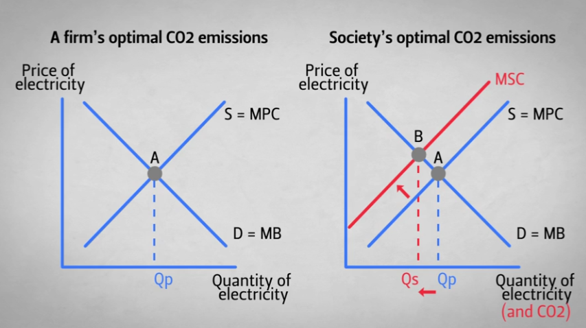
Climate change impacts not only physical but also biological and human systems. Possible impacts of future climate change are important considerations for current decision making, but they are associated with uncertainties. In this chapter we will discuss future projections with climate models, the main sources of uncertainty for those projections, and some global scale impacts.
Prediction is difficult, especially about the future. This is also true for projections of future climate change. They rely on assumptions about future radiative forcings such as anthropogenic emissions of greenhouse gases and aerosols, which are unknown. For this reason they are called projections and not predictions.
Climate scientists believe that the best projections consider results from state-of-the-science climate models because they are syntheses of theoretical and empirical knowledge. However, as we have learned in the previous chapters, climate models are imperfect. Uncertainties in future projections will therefore arise from both, assumptions about future greenhouse gas emissions and climate model errors.
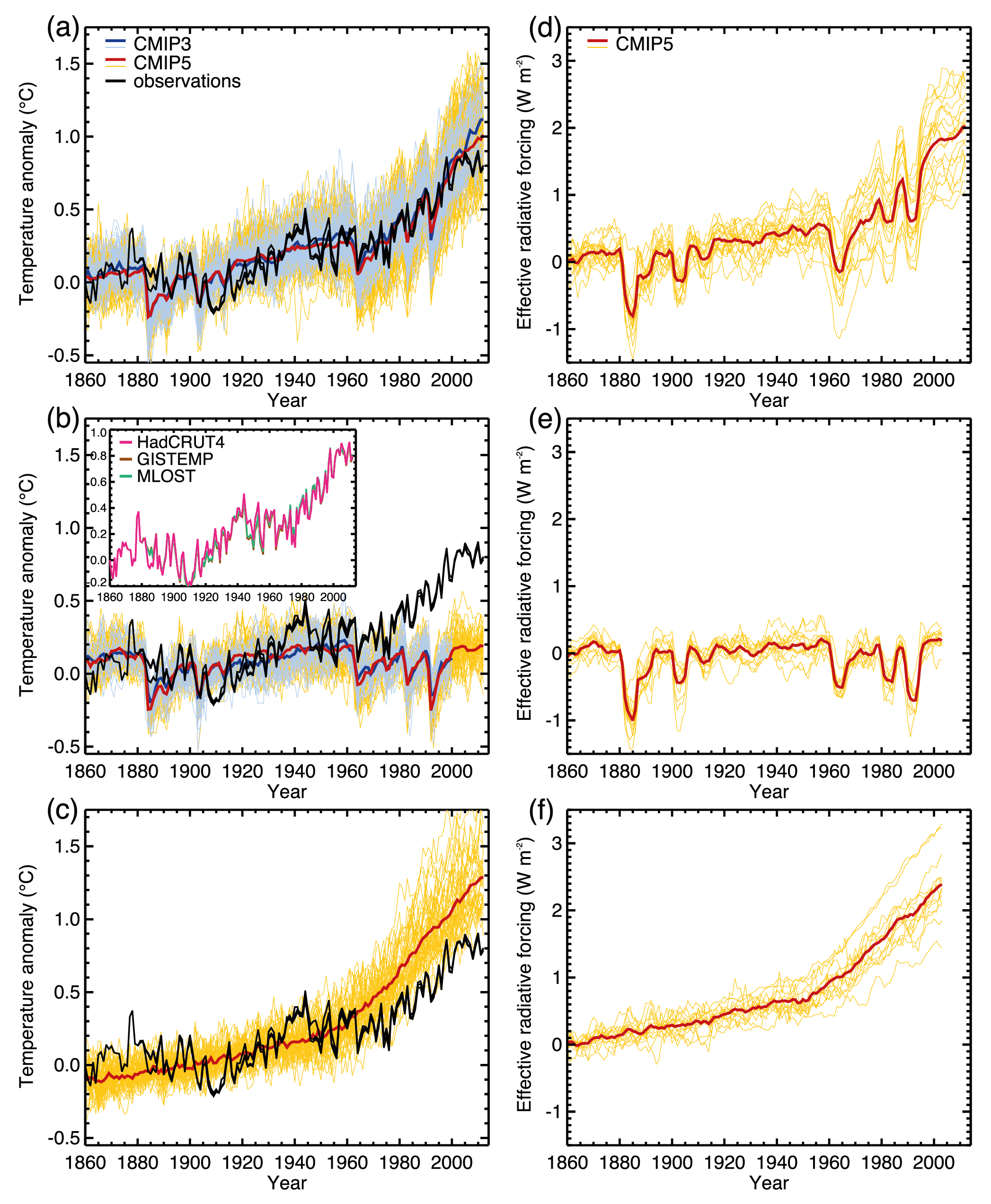
The most recent IPCC assessment report (AR5) uses future scenarios that specify anthropogenic radiative forcing (Fig. 1; Collins et al., 2013; Stocker et al., 2013). They are called Representative Concentration Pathways (RCPs) and are followed by a number that indicates the radiative forcing around year 2100. The goal is to cover a range of possible futures. Note that the radiative forcing slowly decreases after the year 2050 for scenario RCP2.6. In this case the maximum forcing of ~2.5 Wm-2 is reached during the middle of this century. Scenarios RCP4.5 and RCP6.0 continue to increase the radiative forcing during this century and stabilize close to their maximum around year 2100, whereas for scenario RCP8.5 the forcing continues to increase until about year 2200 after which is stabilizes at 12 Wm-2.
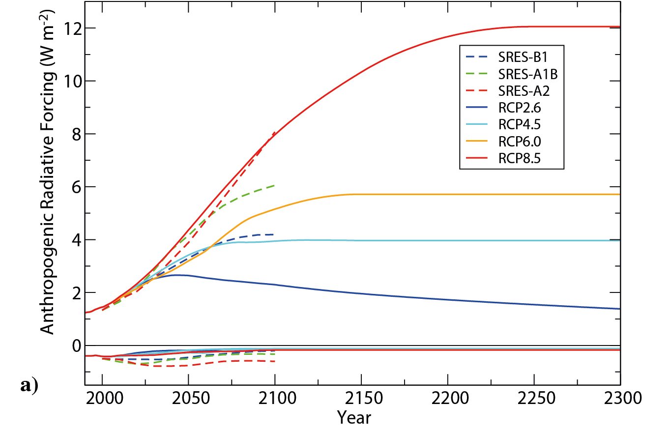
Figure 1: Anthropogenic radiative forcing as a function of time for the current (RCP) and previous (SRES) IPCC scenarios. From
ipcc.ch.
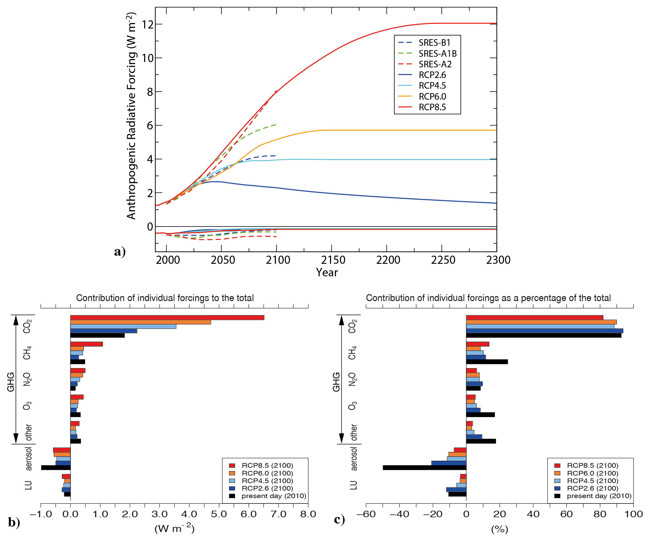
The prescribed radiative forcing is then used to calculate corresponding CO2 concentrations (Fig. 2), e.g. by inverting eq. (2) in chapter 4. Scenario RCP2.6 leads to a stabilization of CO2 concentrations below 450 ppm during the 21st century, whereas in scenarios RCP4.5 and RCP6.0 CO2 concentrations continue to increase to about 550 ppm and 650 ppm, respectively, at year 2100. In scenario RCP8.5 CO2 concentrations increase to about 900 ppm at year 2100. For the upcoming AR6 different scenarios, called Shared Socioeconomic Pathways or SSPs, have been developed.
Carbon cycle models are used to calculate carbon emissions consistent with those CO2 concentration pathways. Due to uncertainties in the models a range of carbon emission scenarios emerges (shaded bands in Fig. 2). Scenario RCP2.6 implies strong reductions in carbon emissions after about year 2020, whereas the business-as-usual scenario RCP8.5 assumes continued increases in emissions until the year 2100 (Fig. 2). The two intermediate scenarios RCP4.5 and RCP6.0 assume continued increases in emissions until about 2050 or 2080 followed by emissions reductions.
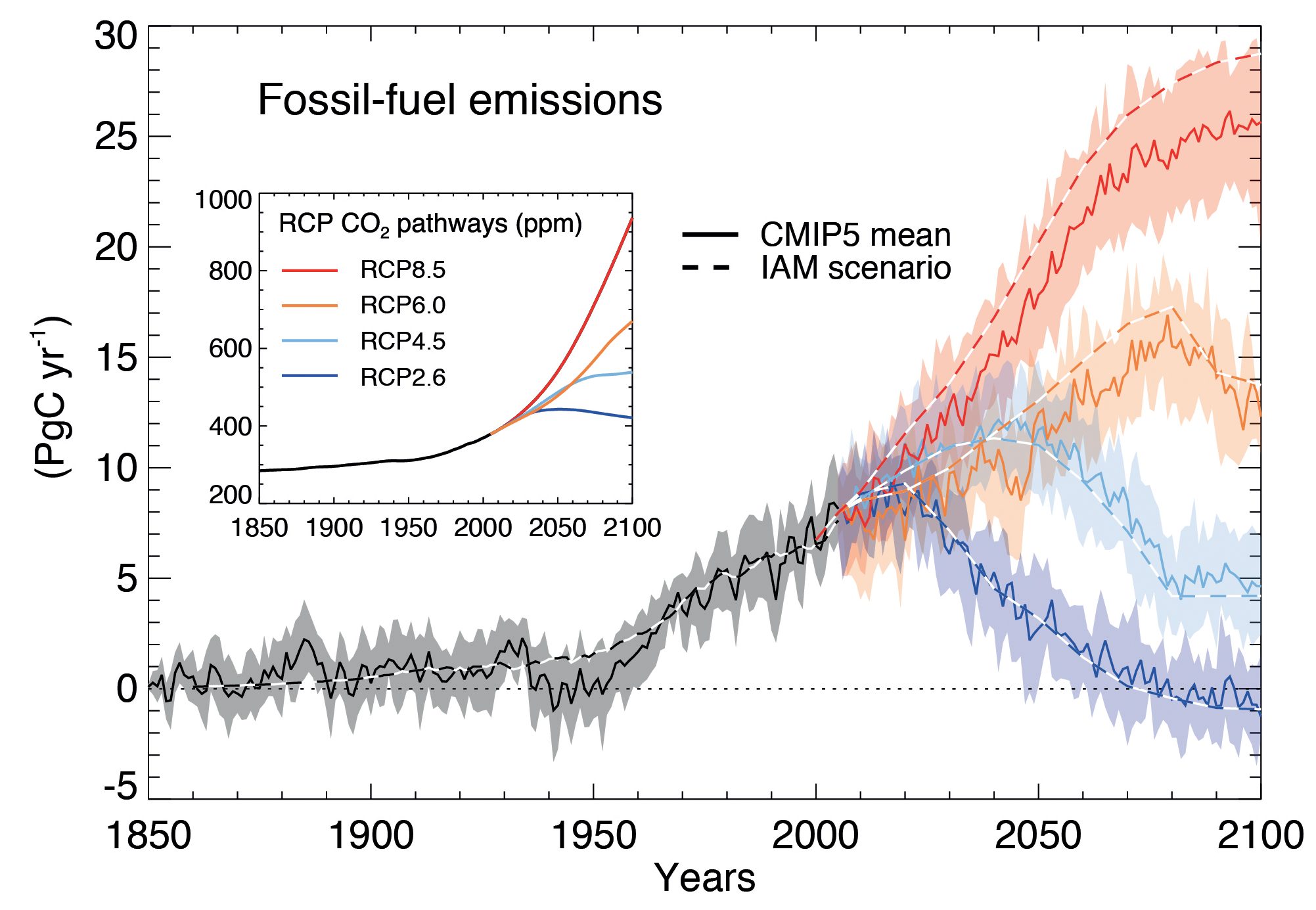
Figure 2: Evolution of CO
2 emissions and concentrations (inset) for RCP scenarios. Emissions are calculated from simple carbon cycle box models given the CO
2 concentrations. Uncertainties in these calculations are indicated by the shading and the two different lines labeled CMIP5 mean and IAM scenario. From
ipcc.ch.
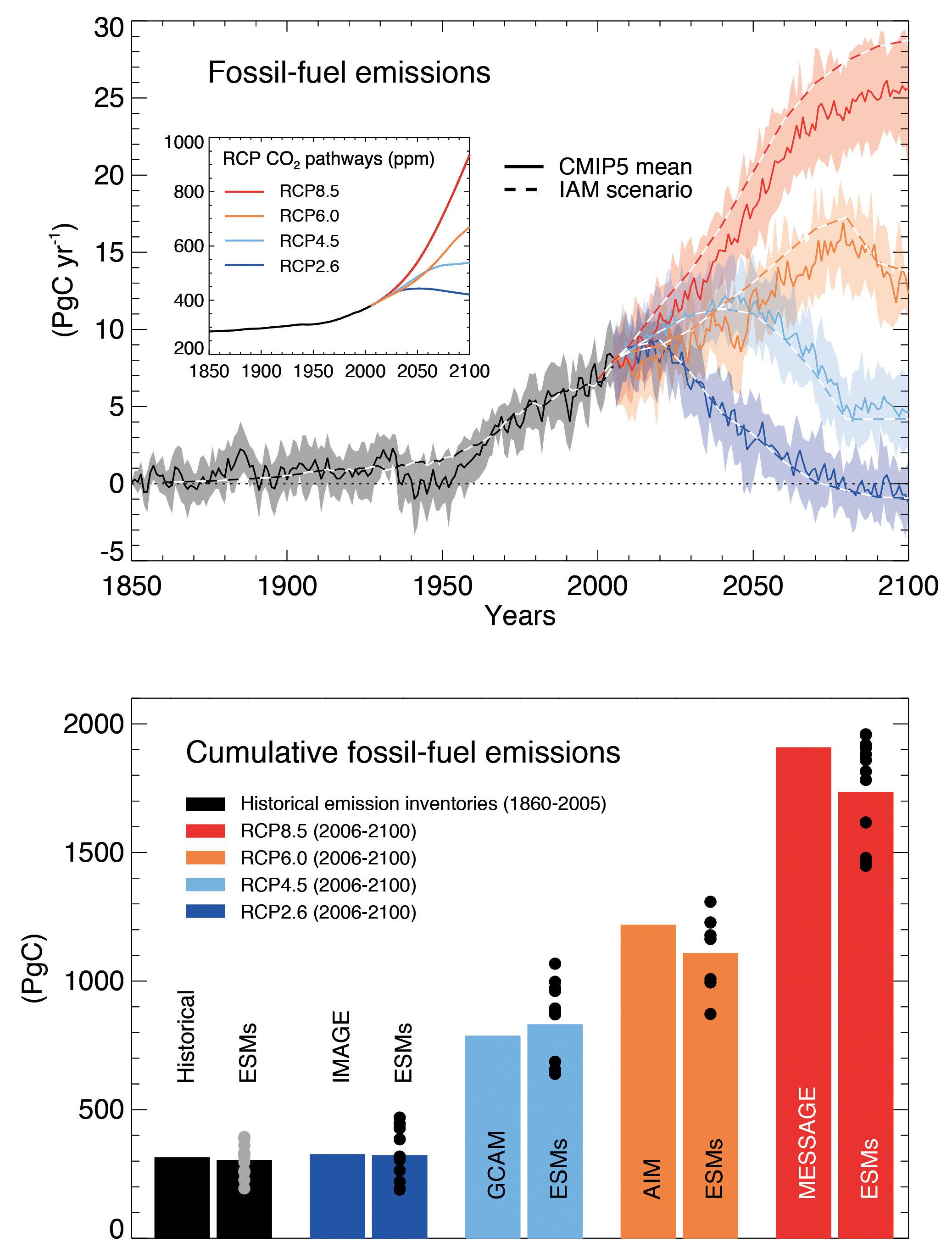
The CO2 concentration pathways are used as input to comprehensive climate models, which project a range of global temperature responses (Fig. 3). For scenario RCP2.6 the models project further warming of less than 1°C above current levels by year 2050 and subsequent slow cooling. Scenarios RCP4.5 and RCP6.0 result in additional warming of about 1.5 to 2°C until year 2100, whereas for the business-as-usual scenario RCP8.5 temperatures increase by 4°C by the year 2100 and by 8°C by year 2300. The latter corresponds to twice the temperature difference between the Last Glacial Maximum and the pre-industrial (see chapter 3). Note that the uncertainty as indicated by the shading is much larger for the high emission scenario RCP8.5 compared with the intermediate and low scenarios.
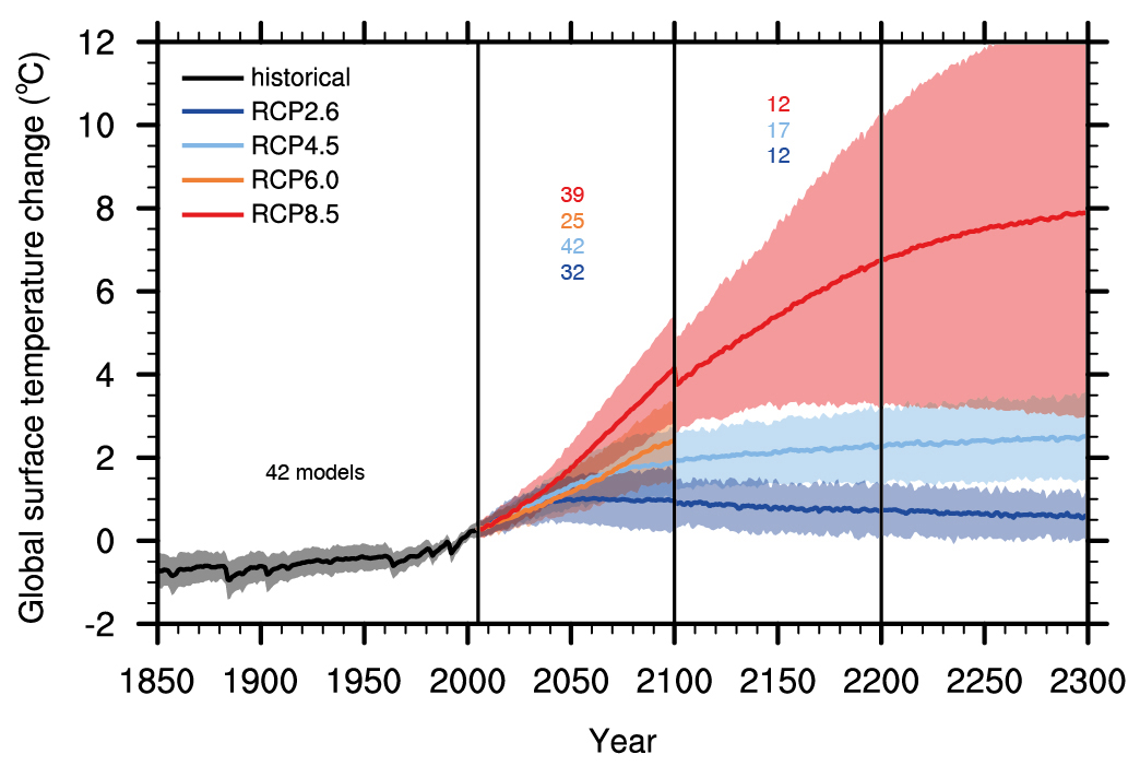
Figure 3. Global average surface temperature projections relative to 1986-2005. Shading indicates the 5 and 95% range and the line is the multi model mean. The black line with the grey shading represents historical simulations including variations in volcanic forcing. Since volcanic forcing is impossible to predict for the future, changes in natural radiative forcings are not considered in the projections. The number of climate models used is indicated. Not all models have simulated the full period until year 2300, which leads to a jump in the red line at year 2100. From
ipcc.ch.
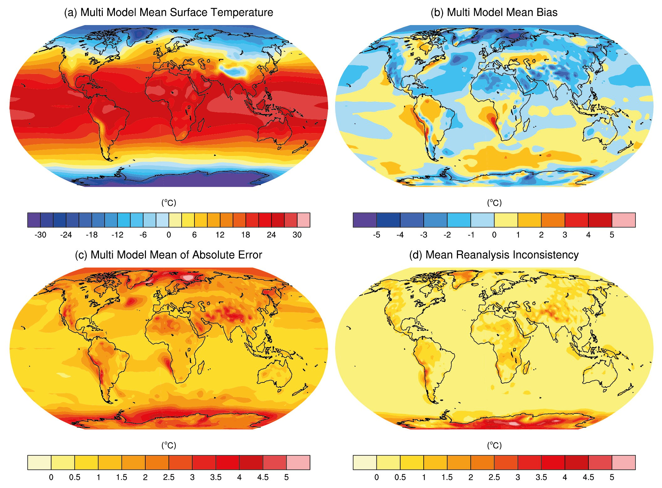
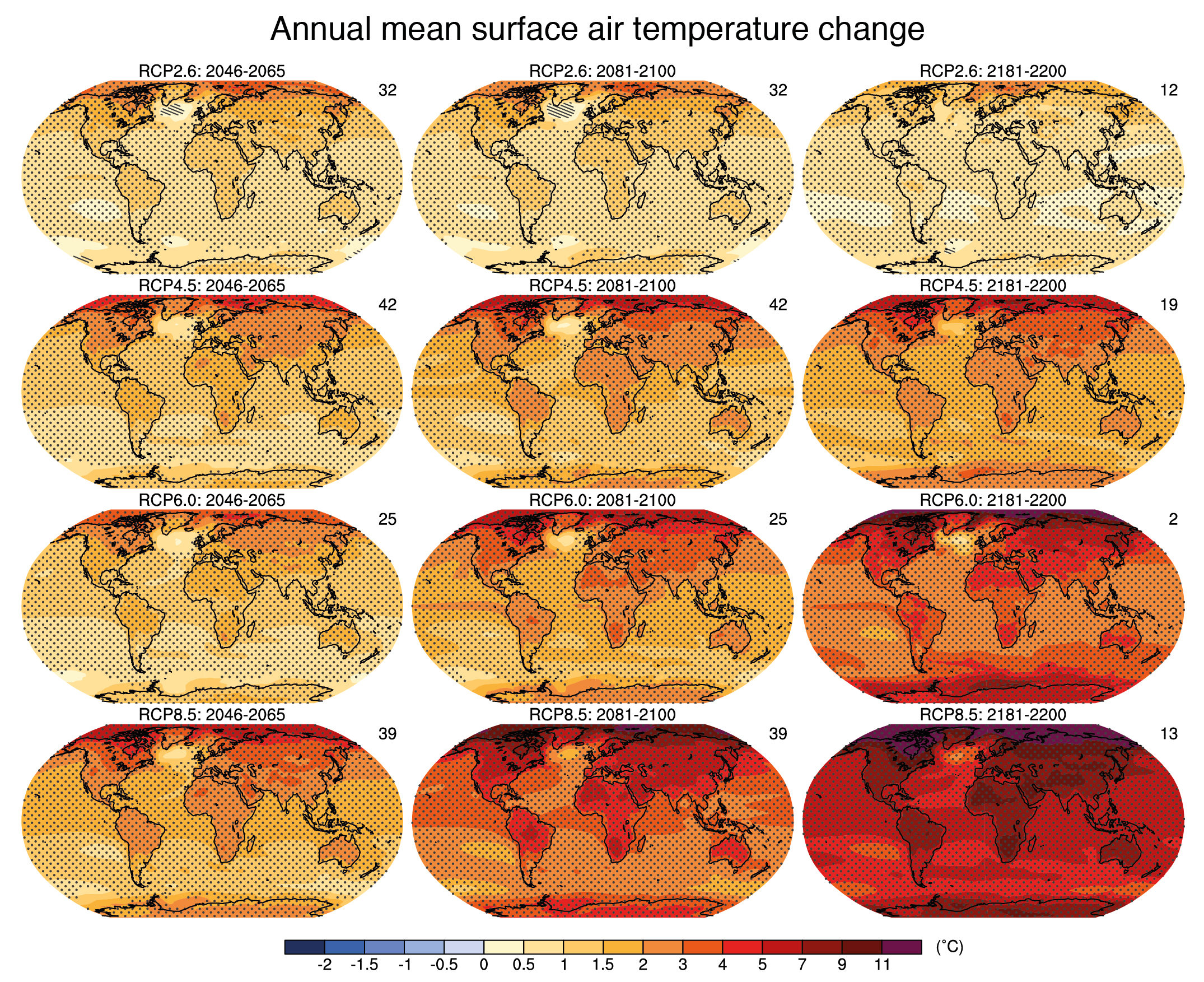
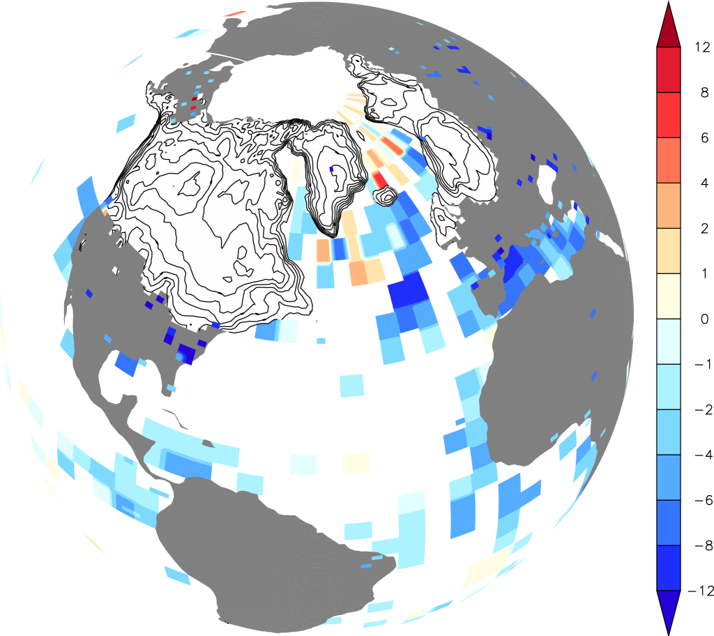
The climate models project more warming over land than over the ocean and more warming at high latitudes, especially in the Arctic (Fig. 4). This pattern is similar for all scenarios and time periods. However, the absolute numbers are smaller for lower emission scenarios than for the business-as-usual scenario RCP8.5 shown in Fig. 4. We have encountered these patterns of land-sea contrast and polar amplification before in the observations of historical temperature changes discussed in chapter 2, in reconstructed temperatures from the Last Glacial Maximum discussed in chapter 3, and in our discussions of detection and attribution studies in chapter 7. We conclude that these patterns are robust features of the climate system that are relatively well understood and reproduced in models. Warming in the Arctic is more than twice as much as the global average, which is dominated by the oceans. The IPCC concludes that, on average, warming over land will be 1.4 to 1.7 times larger than warming over the ocean (Collins et al., 2013).
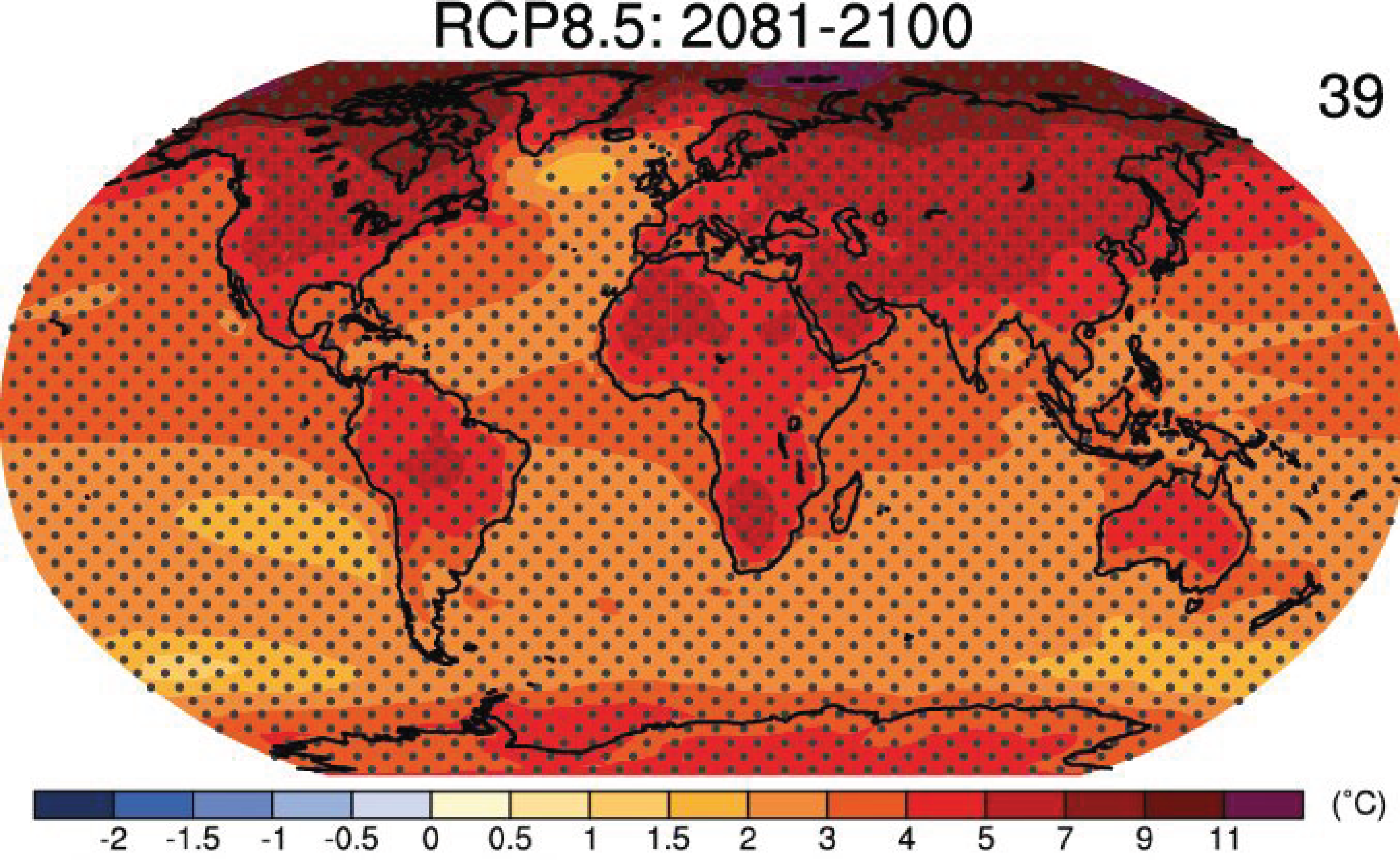
Figure 4: Surface temperature changes projected for the business-as-usual scenario RCP8.5 at the end of the 21
st century. Stippling indicates regions of highly significant changes, where the multi model mean is larger than two standard deviations of modeled internal variability and where at least 90% of models agree on the sign of the change. Click on the map to see projections for other scenarios and times. From
ipcc.ch.
Explore Projections
Explore projections of future climate using this website:
- Select a country, variable and model of your choice.
- How does the model simulation of the seasonal cycle (lower left plot) for the 1980-2004 period compare with the observations?
- Try a different model and then the model mean. Which agrees better with the observations?
- Compare simulations of temperature and precipitation with observations. Which fits better?
- Now compare the model simulation of the future (2050-2074) with the recent past (1980-2004). Describe your observations.
Another good website with climate model projections but also other data is climexp.knmi.nl.
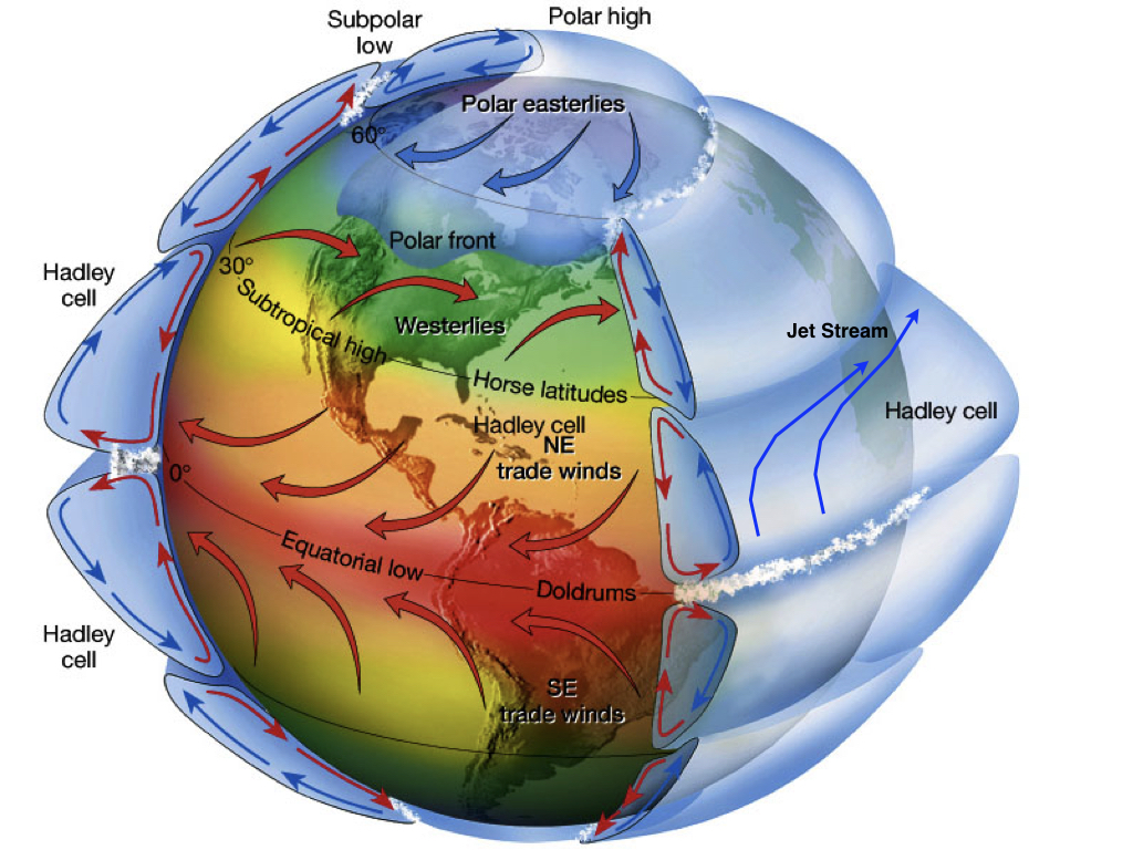
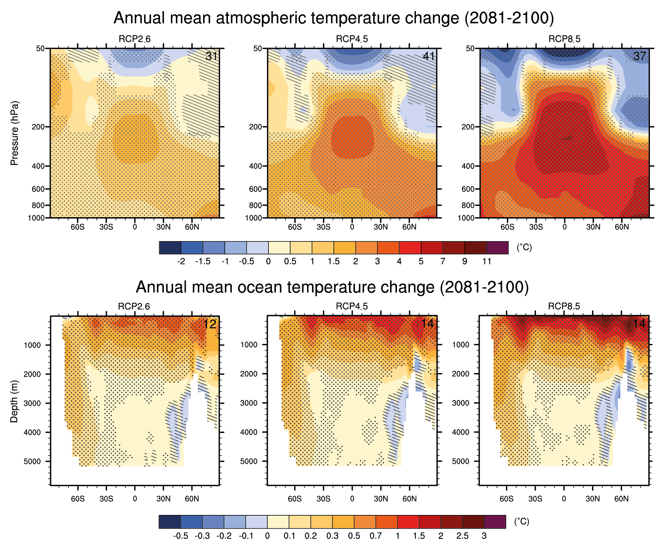
Fig. (5) shows that models project more warming in the upper tropical troposphere than at the surface. Increased water vapor content in the warmer atmosphere (see discussions in Chapter 4 of the Clausius-Clapeyron relation and the lapse rate feedback, and in Chapter 6 of the hydrological cycle) causes more upward moisture transport in the ascending part of the Hadley cell. Enhanced condensation and latent heat release leads to intensified warming there.
Models also project significant cooling in the stratosphere. Since the stratosphere is stably stratified (there is no convection) its energy balance is determined by local heating from the absorption of solar radiation by ozone and local cooling from the emission of infrared radiation by CO2 (Manabe and Strickler, 1964). Thus, higher CO2 concentrations in the stratosphere will lead to more emission of infrared radiation and cooling there. Stratospheric cooling is observed in contemporary measurements, consistent with the cooling effect of CO2. However, the current cooling is also caused by decreases in stratospheric ozone caused by human emissions of Chlorofluorocarbons (CFCs). Nevertheless, the projected stratospheric cooling for the future will be dominated by CO2 increases since CFC emissions have decreased and the ozone hole is expected to heal over the next decades.
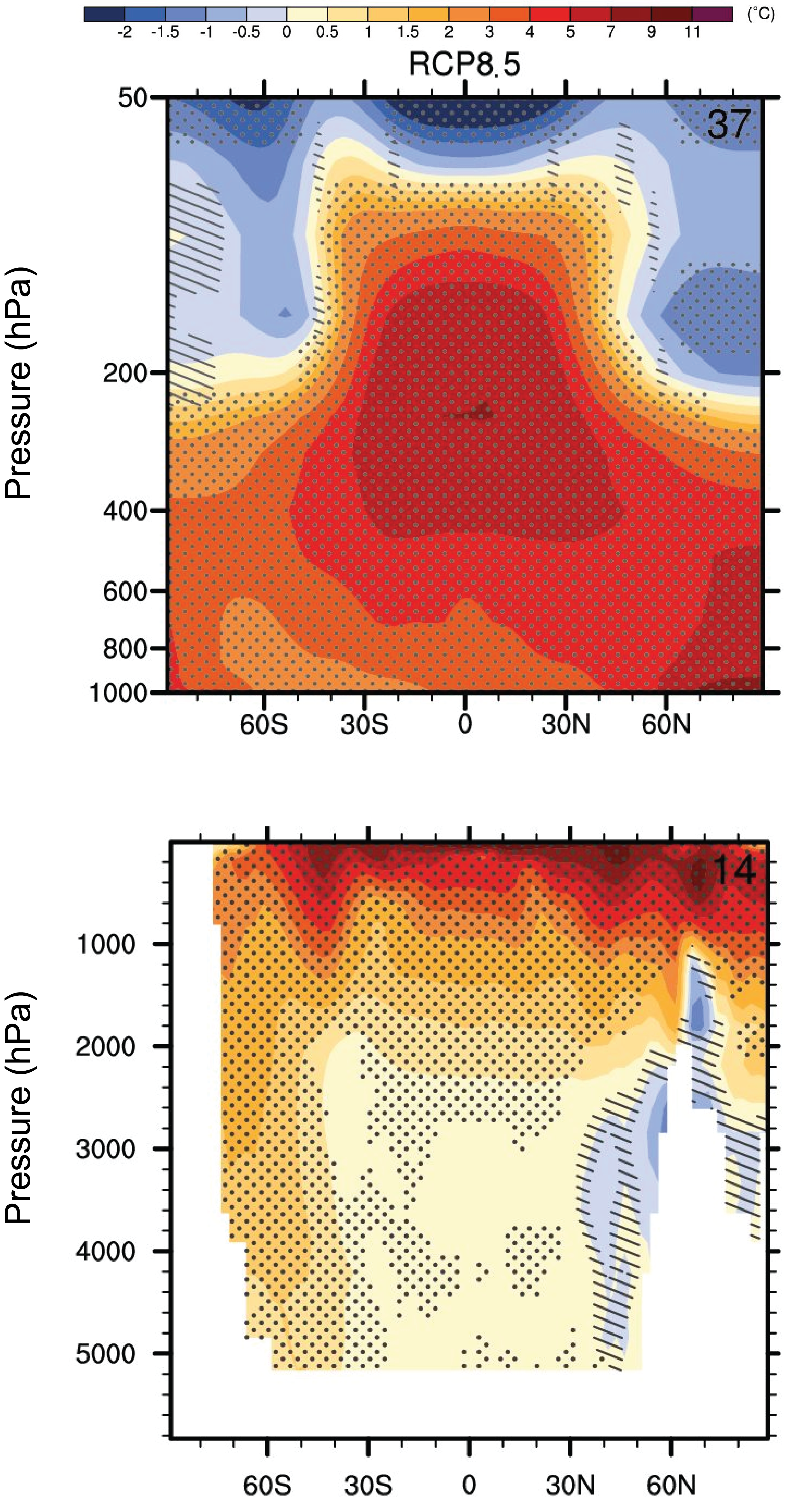
Figure 5: Zonally averaged temperature changes projected for the end of the 21
st century in the atmosphere (top) and ocean (bottom) as a function of latitude and pressure (height, top) and depth (bottom) for scenario RCP8.5. Stippling indicates significance as in Fig. 4. Hatching indicates where changes are not significant with respect to 2 sigma variations of internal variability. Click on the ocean panel to see results for other scenarios. From
ipcc.ch.
The observed warming of the upper ocean is projected to continue and penetrate deeper into the ocean interior particularly in regions of deep water formation such as the Southern Ocean (Fig. 5). More warming of the surface will increase the stratification of the ocean and reduce vertical mixing, with implications for the ocean’s meridional overturning circulation and nutrient delivery to the euphotic zone, both of which will likely continue to decrease.
Warming of the surface is projected to increase evaporation everywhere except in the northern North Atlantic and Southern Ocean where the warming is smallest and over some land areas where precipitation is projected to decrease (Fig. 6). Precipitation is generally projected to increase in regions that are already wet like the tropics and at mid- to high-latitudes, and decrease in regions that are already dry like the subtropics. Relative humidity is generally projected to decrease over land areas and increase over the oceans. The net surface freshwater loss, which is determined by evaporation minus precipitation (E − P), is projected to increase in the subtropics, whereas the tropics and mid- to high latitudes will gain water. Runoff is projected to increase in most regions except around the Mediterranean, the Southwest US and Mexico, southwest Africa, and parts of South America. Soil moisture, on the other hand, is projected to decrease almost everywhere except in parts of North Africa, Asia, and South America, where precipitation increases substantially.
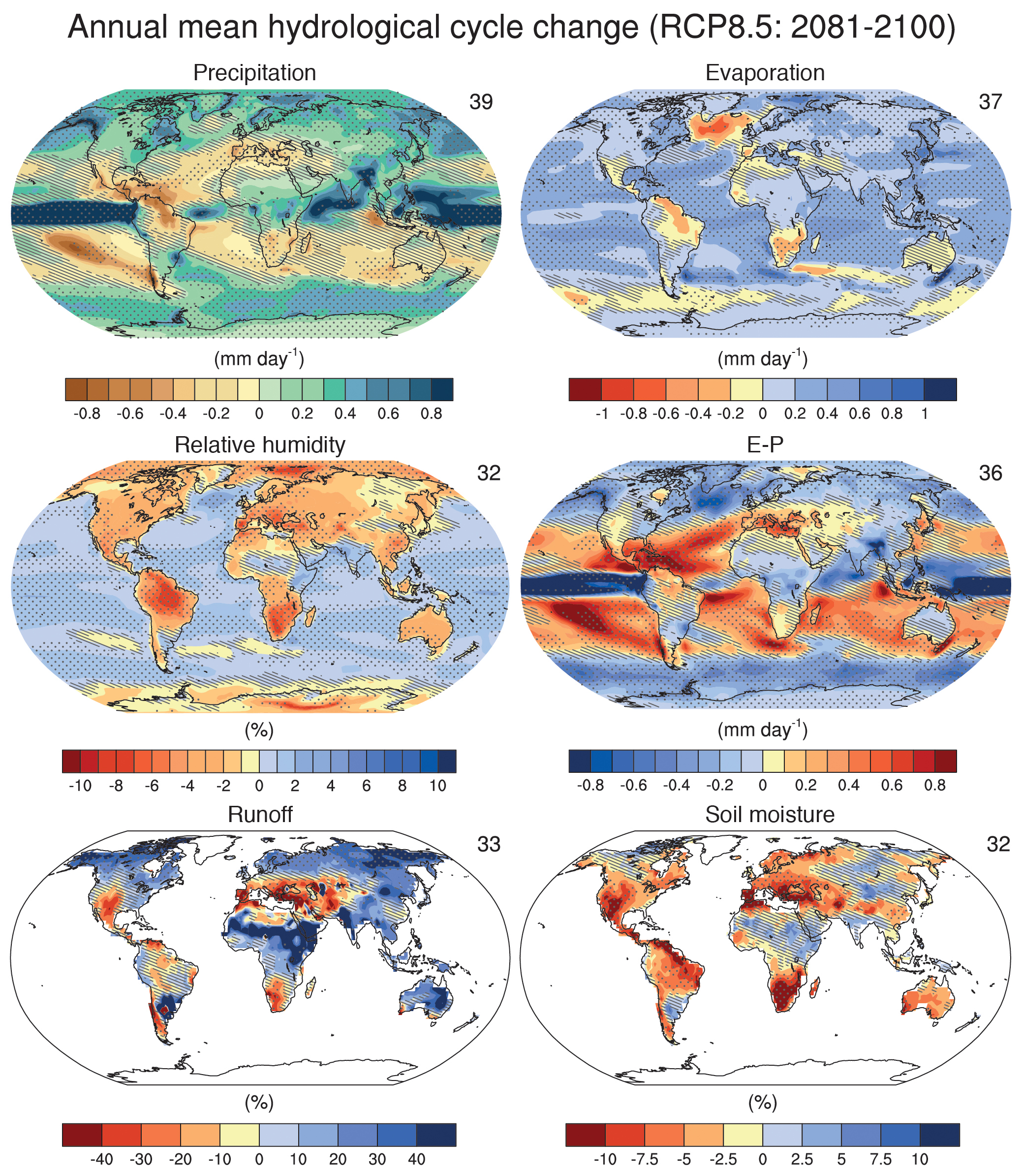
Figure 6: As Fig. 4, but for changes in the hydrological cycle. From
ipcc.ch.
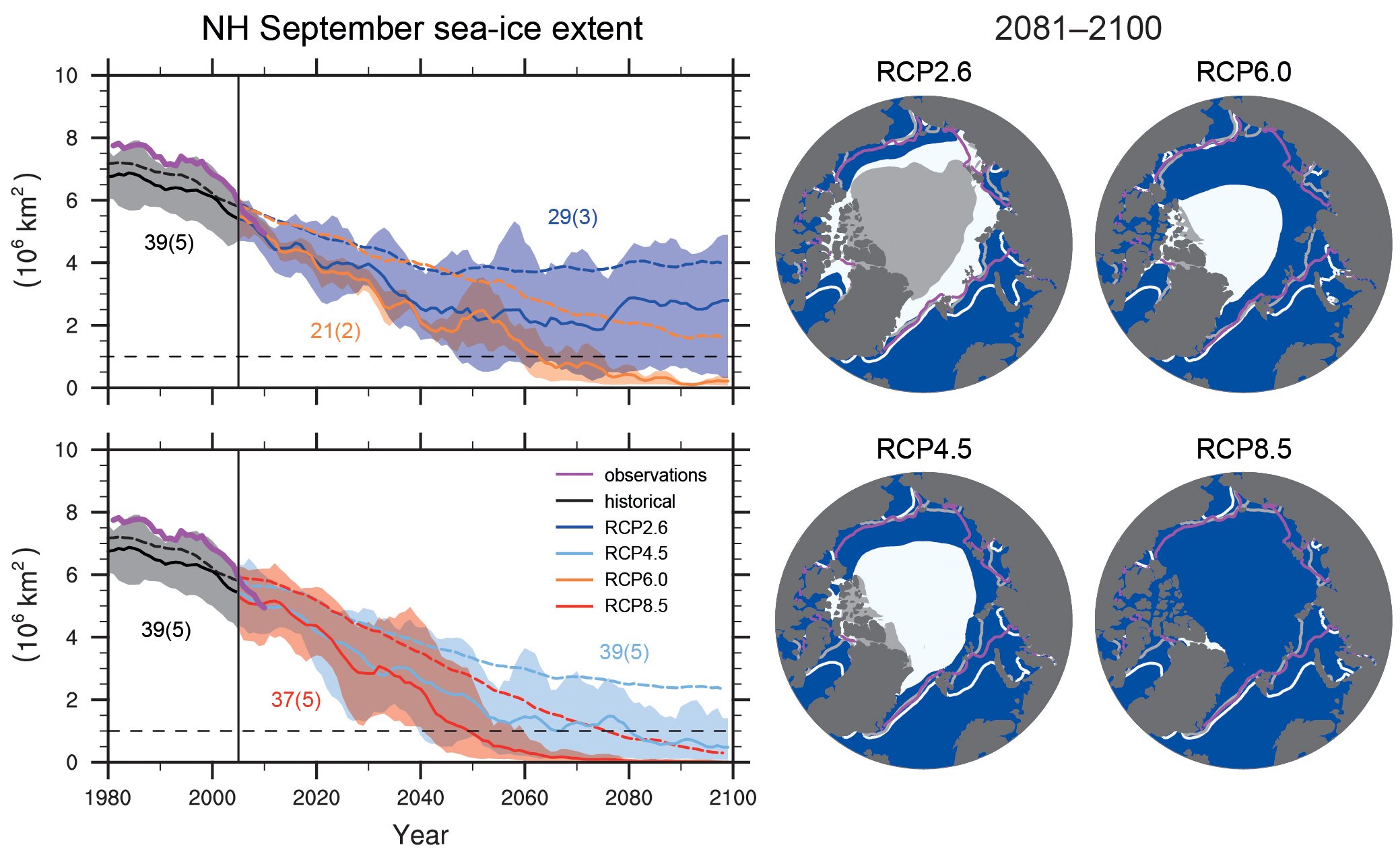
Projections suggest that Arctic sea ice will continue to decline in the future particularly at the end of summer (Fig. 7). However, much larger declines are projected for the high emission scenario (RCP8.5), for which all models project an almost completely ice free Arctic ocean, compared to the low emission scenario (RCP2.6), for which all models project a substantial remaining sea ice cover.

Figure 7: Projections of Arctic sea ice in September. Results from all models are shown as dashed lines in the time series panels on the left and as white shading in the maps on the right. Results from a subset of models that agree best with observed sea ice (numbers in brackets) are shown as solid lines and grey shading. From
ipcc.ch.
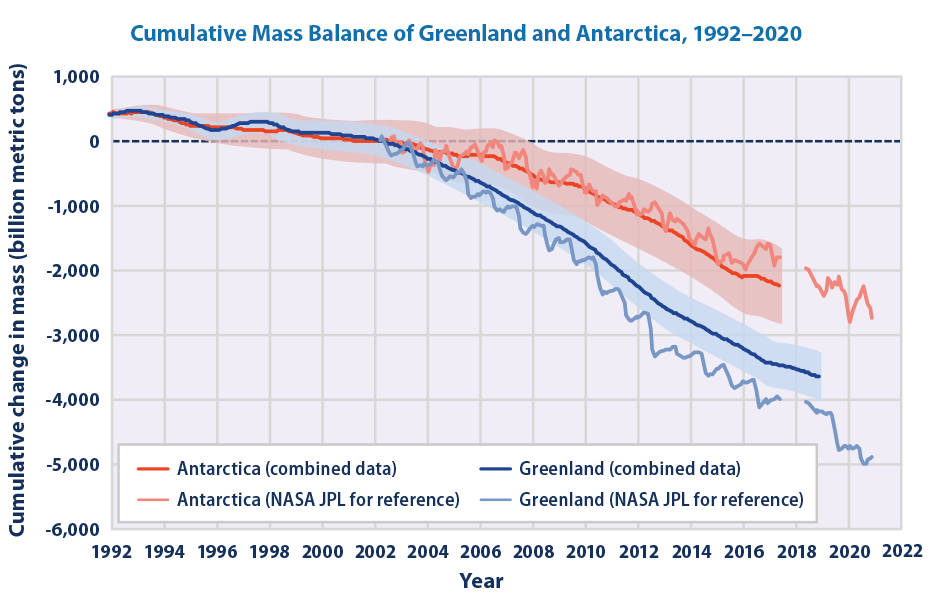
Mountain glaciers are also projected to continue to melt, as well as the Greenland and Antarctic ice sheets. Due to this input of mass together with the expansion of the ocean from warming sea levels are projected to increase by 40 to 70 cm by the year 2100 (Fig. 8). Note that sea level projections are very similar for all scenarios until mid-century. This indicates the commitment to the near future sea level rise from past carbon emissions. In other words, considerable climate change and the associated impacts are already baked into the system and cannot be avoided. It implies the necessity to adapt to these unavoidable impacts.
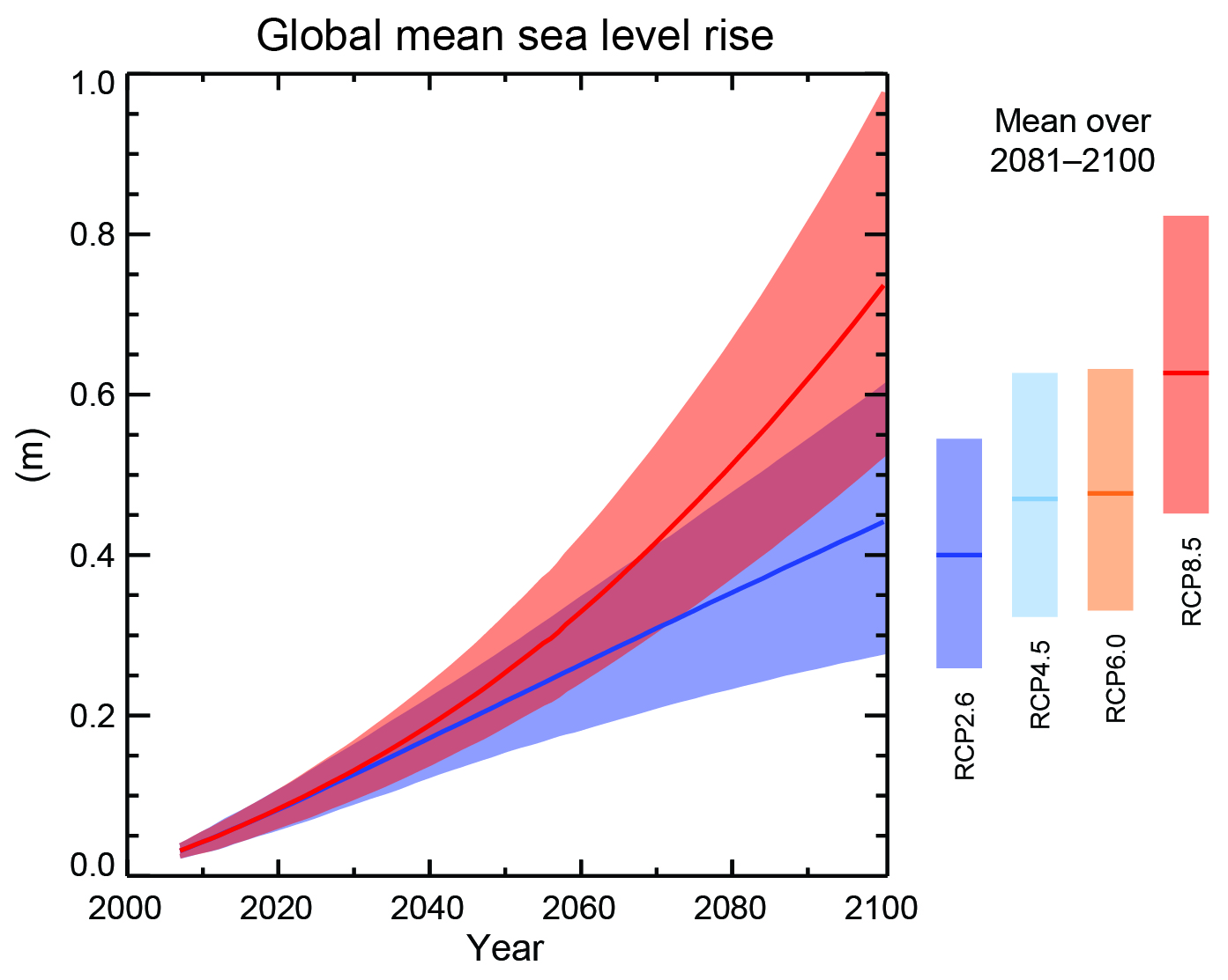
Figure 8: Global sea level rise projected for the 21
st century. The blue and red curves show projections for scenarios RCP2.6 and RCP8.5, respectively. The shading indicates the likely (66-100%) uncertainty range. Bars on the right show the 2081-2000 averages for four scenarios. From
ipcc.ch.
Increasing stratification from warming and freshening of North Atlantic surface waters will lead to a slowdown of the Atlantic meridional overturning circulation, by about 10% for each degree Celsius global mean warming (Bakker et al., 2016). Many other impacts also depend approximately linearly on global mean temperature and global mean temperature can be well approximated by cumulative carbon emissions (Matthews et al., 2009) such that 500 Gt lead to approximately 1°C of warming (Fig. 9). Since we’ve already emitted about 500 Gt, this means that if we want to stay below 2°C, the goal of the Paris Agreement, we have only another 500 Gt of carbon to emit.
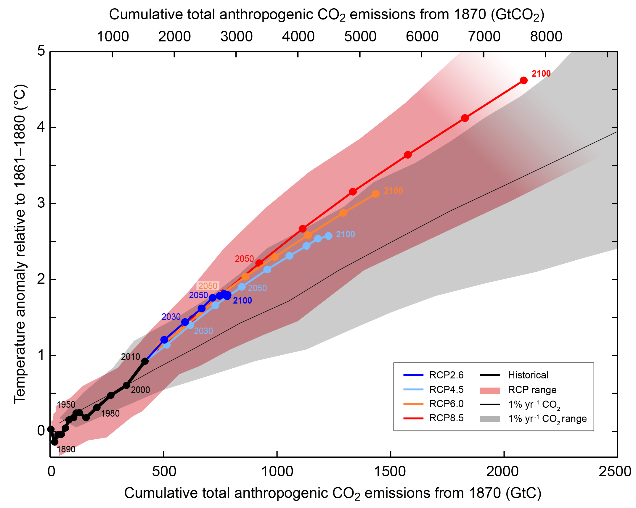
Figure 9: Global mean surface temperature change as a function of the cumulative anthropogenic carbon emissions. Cumulative carbon emissions are the area under the curves in Fig. 2. Colored lines show multi-model means from the RCP scenarios and colored plume indicates uncertainties. Results from exponential CO
2 increase experiments at a rate of 1% per year are shown as the black line and grey shading. RCP scenarios lead to somewhat larger warming because they include additional non-CO
2 forcings. From
ipcc.ch.
Box 1: Tipping Points
A tipping point is a threshold that when crossed will lead to an irreversible transition into a different state. Examples for tipping points are
- melting of the Greenland ice sheet,
- melting of the West Antarctic ice sheet,
- collapse of the Atlantic meridional overturning circulation,
- ecosystem shifts,
- species extinctions.
Ice sheets can have tipping points due to positive feedbacks, such as the ice sheet elevation – mass balance feedback (Weertman 1961). This feedback can be understood by considering an idealized ice sheet on a flat bed as illustrated in Fig. B1.1 below. An ice sheet gains mass through accumulation of snow in the upper central parts, whereas it looses ice through melting along the lower-lying margins. For simplicity we assume in the following that the accumulation and melt rates are spatially constant. Due to gravity and the resulting horizontal pressure gradient the ice flows slowly from the center towards the margins. Moving upward on a glacier or ice sheet one starts at the margin to walk on ice. At some point the ice turns into snow, which covers the interior of the sheet all the way to the summit. This is the so-called snow line or equilibrium line. It indicates the transition from the melt-zone to the accumulation zone. If the mean height of the ice sheet  is larger than the height of the equilibrium line HE the ice sheet is in a stable equilibrium. However, if warming temperatures rise the equilibrium line to the ablation area increases and the ice sheet looses more mass than it gains. It shrinks and its height drops, which leads to even more melting. This feedback can lead to a rapid and irreversible melting of an entire ice sheet.
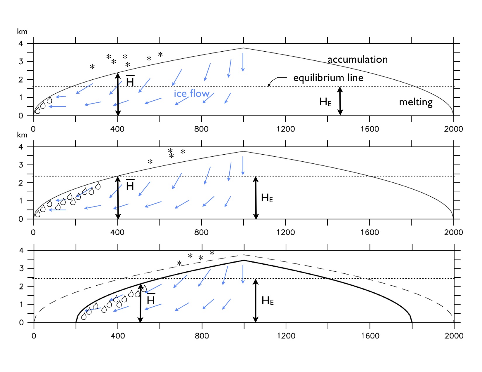
Figure B1.1: Schematic section across an idealized ice sheet. The horizontal axis represents the distance in km from its left margin. The vertical axis represents elevation above the flat base.
As a result of this feedback ice sheets exhibit hysteresis behavior as illustrated schematically in Fig. (B1.2). If the height of the equilibrium line is between zero and two states are possible. One without ice and one with an ice sheet. Assume we’re in a state without ice on the lower branch of the hysteresis curve. If the climate cools and the equilibrium line drops below zero ice will grow and we will switch to the state with an ice sheet. If the climate now warms again the ice sheet will stay in place until the height of the equilibrium line raises above . At this point the ice sheet will melt. So, for equilibrium line heights between zero and two states are possible and which state the system is in depends on its history. This is a typical property of hysteresis as observed e.g. in magnetism. It also can lead to rapid changes in state as illustrated by the vertical arrows. Due to its latitude being further poleward and its height being higher it is thought that the East Antarctic ice sheet is more stable and further away from the melting threshold than the Greenland ice sheet.
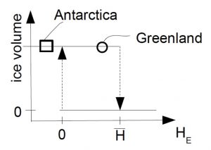
Figure B1.2: Schematic hysteresis curve for an ice sheet. The vertical and horizontal axes represent ice volume and height of the equilibrium line, respectively.
More complex ice sheet models exhibit similar threshold behavior. Current estimates suggest that the Greenland ice sheet may disappear almost completely for global warming of 0.8-3.2°C above pre-industrial temperatures (Fig. B1.3). However, even though this threshold may be exceeded in the near future due to continued anthropogenic carbon emissions, the ice sheet will not disintegrate immediately. It may take hundreds to thousands of years to melt completely. The larger the warming the more rapid the ice melt will be. Melting of the entire Greenland ice sheet would raise global sea level by about 7 m.
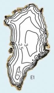 |  |
| Figure B1.3: Greenland fully glaciated (left) and mostly deglaciated (right). Contour lines denote ice sheet thickness in km. From Robinson et al. (2012) at nature.com. |
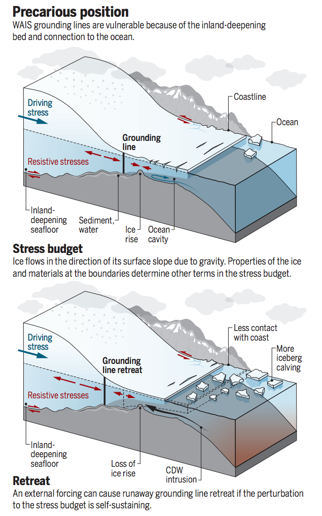
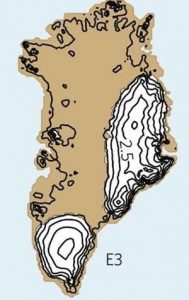
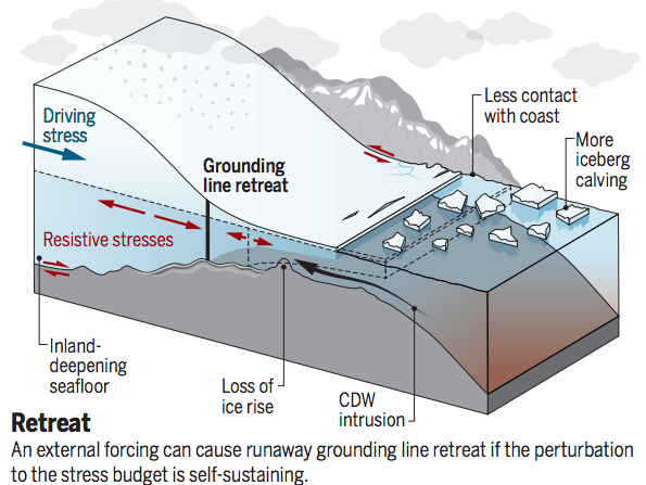
The West Antarctic ice sheet is also vulnerable to warming. Most of it is below sea level and it is fringed with ice shelves that float on the ocean (Fig. B1.4). The grounding line separates the ice shelf from the grounded inland ice. Ice shelves often provide a buttressing force that keeps the interior ice sheet from flowing faster into the ocean. Warm Circumpolar Deep Water (CDW) intrusion can melt the bottom of the ice shelf, increase calving of ice bergs and lead to retreat of the grounding line. Because the deepening of the bed towards the interior retreat of the grounding line and reduced buttressing can cause an increase in the outward ice flow and initiate an instability that leads to the collapse of the entire ice sheet. Recent models indicate that the West Antarctic ice sheet could disintegrate within hundreds of years for high and intermediate carbon emission scenarios, whereas it is stable for low emission scenarios (DeConto and Pollard, 2016). If the West Antarctic ice sheet collapsed global sea level would rise by about 5 m. Here is a short video about this topic.
 |
 | 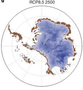 |
| Figure B1.4: Antarctic ice sheet vulnerabilities. Top: Schematic illustration of the West Antarctic ice sheet from carbonbrief.org. Bottom: Projection of the Antarctic ice sheet at year 2500 for emission scenarios RCP2.6 (left) and RCP8.5 (right) from DeConto and Pollard, 2016). |
The Atlantic Meridional Overturning Circulation (AMOC) also has the potential to switch into a collapsed state once a threshold is exceeded. Paleoclimate evidence indicates that such shifts happened repeatedly in the past. The AMOC exhibits hysteresis behavior because of a positive feedback between the circulation and salinities in the North Atlantic. The circulation transports high saline waters from the subtropics towards the North Atlantic. However, a reduction of the flow and thus the northward transport of saline waters will lead to decreasing salinities in the North Atlantic regions of deep water formation and this will reduce the flow even further. Currently it is thought that an AMOC collapse is unlikely for low emission scenarios but the probability increases for high emission scenarios (Bakker et al., 2016). A collapse or large reduction of the AMOC would impact not only the North Atlantic due to reduced northward heat transport, it would also affect the tropics by shifting the Intertropical Convergence Zone towards the south, which would affect precipitation patterns, vegetation, ecosystems and humans there and it would affect ocean biogeochemical cycles (e.g. of nutrients and carbon) and ecosystems.
Ecosystems will continue their poleward and upward shifts. Present day tundra, for example, will be replaced by taiga (Fig. B1.5). Species that used to live at high latitudes or on the upper elevations of mountains may be replaced by species moving in from further south or from lower altitudes. This can lead to species extinctions. Especially vulnerable are species that live near the top of mountains such as the cute little pika, or near disappearing sea ice such as polar bears, walrus, and narwhales (Larsen et al., 2014).
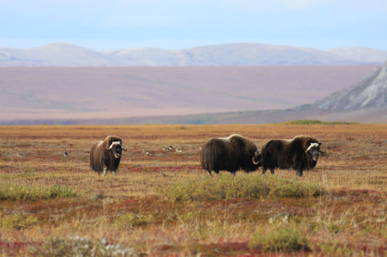 | 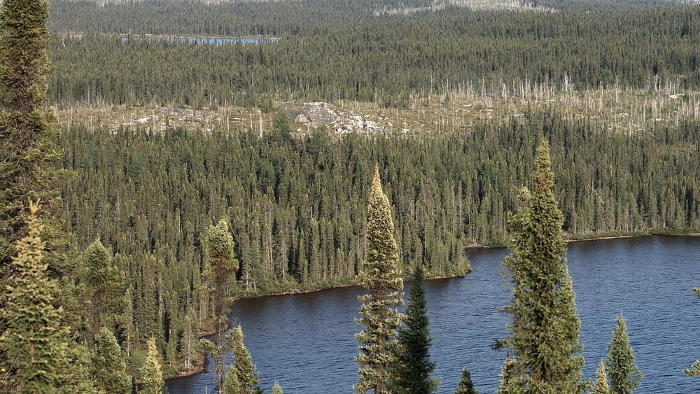 |
| Figure B1.5: Tundra (left) is a biome at far northern latitudes characterized by grasses and shrub vegetation and permafrost beneath the seasonally thawed soil. Musk oxen, geese, caribou (reindeer), Arctic fox, Arctic hare, snow owl, and lemmings are some of the animals that call the tundra home. Warming leads to taiga (a.k.a. boreal forest, right) with coniferous trees replacing the tundra. |
Vegetation models project further poleward shifts in biomes (Fig. 10) due to warming consistent with the currently observed ongoing trends. Potential vegetation is the natural vegetation that would grow in a certain area without human land use changes such as agriculture or forestry. The biome shifts are projected with the most confidence in those regions close to the biome boundaries towards the migration direction of the invading biome. E.g. close to the tundra/taiga boundary there will be almost certainly a shift from tundra to taiga. For individual species such as aspen in North America large shifts are possible.
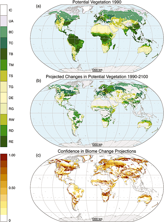
Figure 10: Modeled potential vegetation in 1990 (a), projected changes by the end of the century (b) and the confidence in the projections (c). Biomes from poles to equator are ice (IC), tundra and alpine (UA), boreal conifer forest (taiga, BC), temperate conifer forest (TC), temperate broadleaf forest (TB), temperate mixed forest (TM), temperate shrubland (TS), temperate grassland (TG), desert (DE), tropical grassland (RG), tropical woodland (RW), tropical deciduous broadleaf forest (RD), tropical evergreen broadleaf forest (RE). From Gonzalez et al. (2010).
Increasing CO2 concentrations in the atmosphere will increase the water-use efficiency of plants. They can grow more with the same water use because they don’t need to open their stomata as much for the same amount of CO2 to flux in. They can also grow in regions that were previously too dry for them under lower CO2. This greening effect is currently observed e.g. from satellites.
Changes in precipitation will also impact vegetation distribution. The effects on vegetation of reduced precipitation in the subtropics in a warmer climate may be compensated to some degree by the increased water-use efficiency under higher CO2. Longer growing season, higher CO2, and warmer temperatures will increase net plant production but also respiration, e.g. in soils.
Wildfires are difficult to project but in most regions they are likely to get worse due to climate change (Fig. 11). Fire needs fuel, which in the case of wildfire is burnable biomass (dry wood or grass). It also needs the right climatic or weather conditions. Hot and dry summers increase fire hazards and strong winds can lead to rapidly spreading fires. In many regions, e.g. North America, Australia and Russia, fire suppression by humans have caused a build up of fuel, which, once ignited, can lead to larger fires. In many parts of the tropics, on the other hand, humans burn to clear agricultural fields. Thus, changes in wildfires are not only caused by climate change. However, hotter drier summers, projected e.g. for the western United States, will lead to increased fire probability in the future. This is consistent with scientific evidence that fires have already increased there in recent decades due to anthropogenic climate change (Abatzoglou and Williams, 2016). In other regions such as the high northern latitudes, where woody taiga vegetation will replace tundra the resulting increase in available fuel may lead to more or larger fires. Note that the changes in projected fire frequency are highly uncertain as indicated by different models and methods yielding different results.
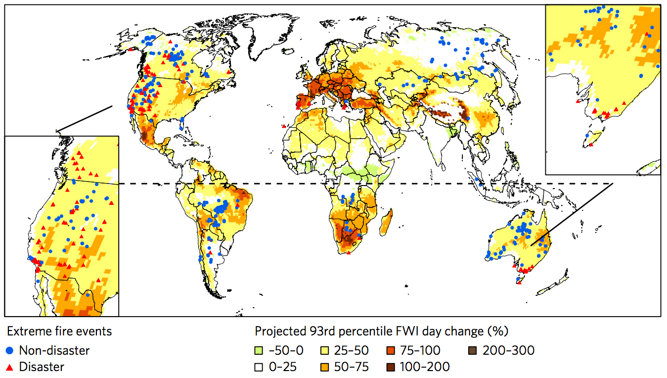
Figure 11: Projected changes in the number of days exceeding the 93rd percentile of the Fire Weather Index (FWI) by the mid 21st century (2041-2070) under a high emissions scenario (RCP8.5). Dark red shading indicates the largest increases, while the pale green shows small decreases. Red triangles and blue dots show recent extreme wildfire events. Source: Bowman et al. (2017). From
carbonbrief.com.
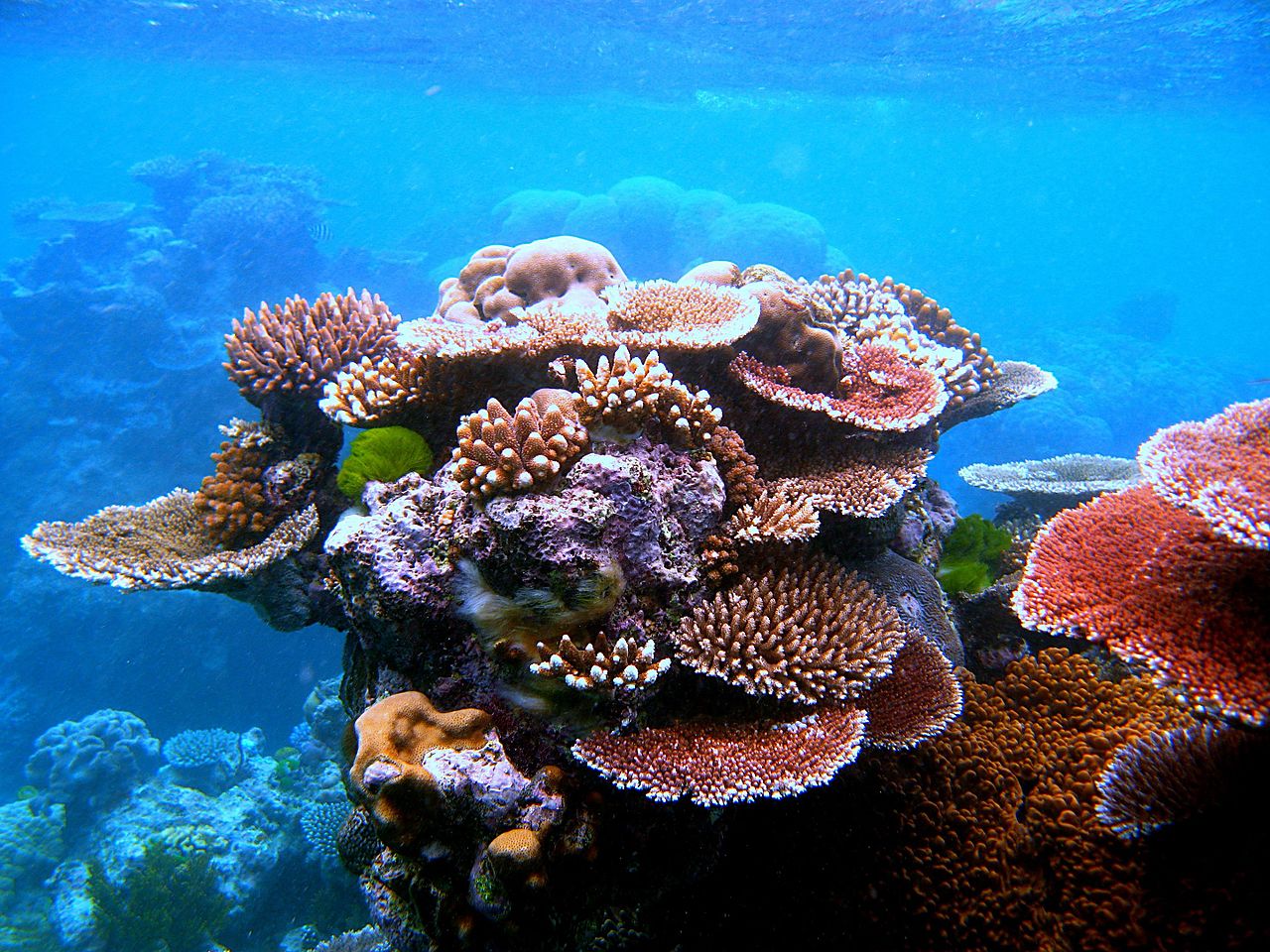
One of the most sensitive ocean ecosystems are probably coral reefs. Corals are threatened not only by bleaching, which refers to the expulsion of their symbiotic algae resulting from warmer waters, but also by ocean acidification, which inhibits their calcium carbonate production. The presently observed shift of fish species towards higher latitudes will most likely continue.
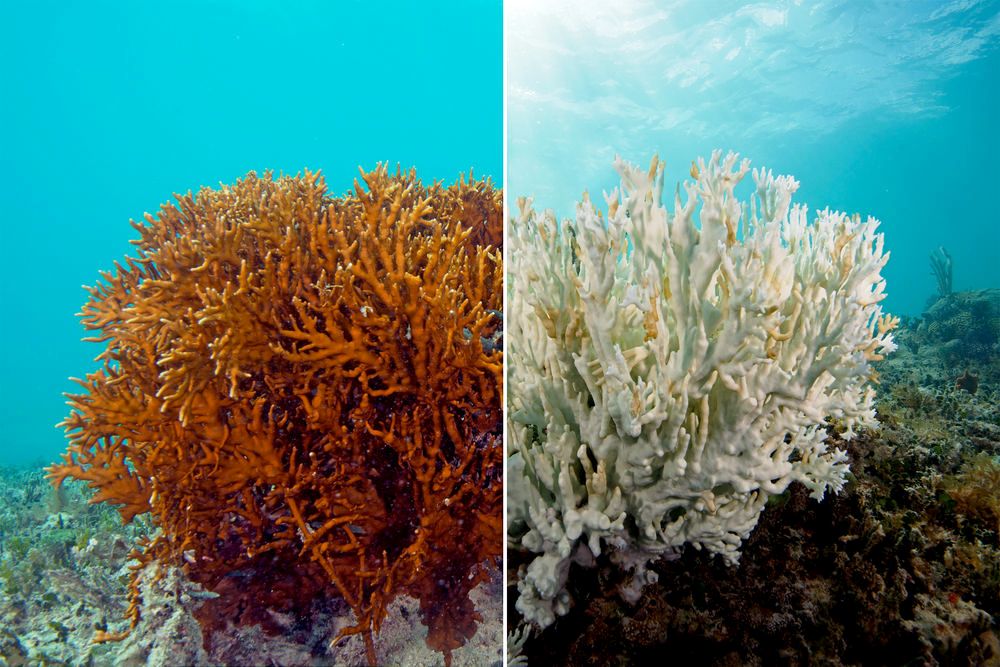
Figure 11: Healthy (left) and bleached (right) coral.
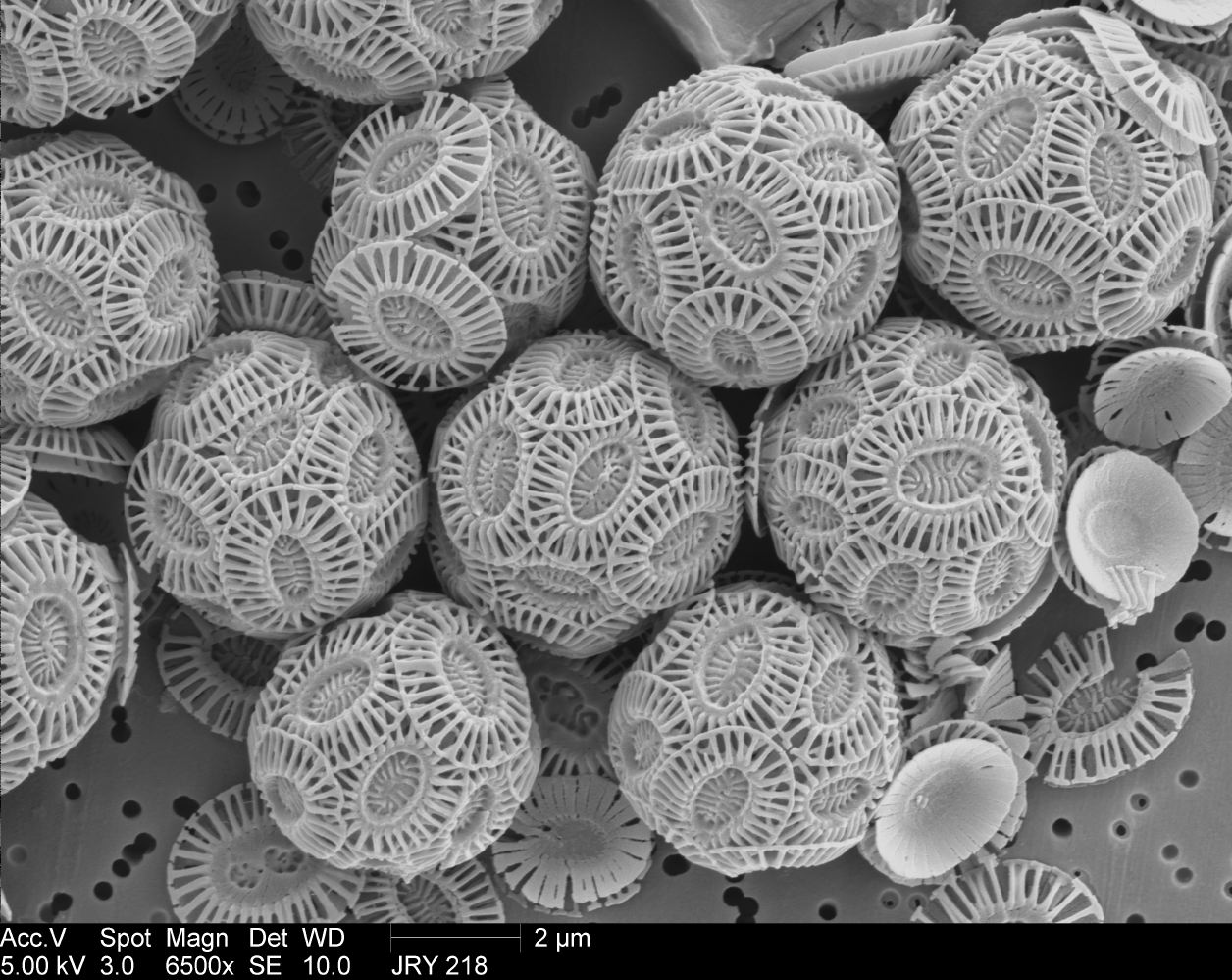
In the Arctic narwhales may be replaced by invading killer whales (Fig. 12). Similarly, for many other species from phytoplankton to whales, some will benefit and others will suffer from climate change. Calcifiers such as coccolithophores will presumably be among the losers due to ocean acidification, whereas cyanobacteria, which is another group of phytoplankton, may be among the winners (Dutkiewitcz et al., 2015). Because of this complex response, many consequences for ecosystems cannot be predicted. It is therefore likely that there will be surprises that scientists could not foresee.
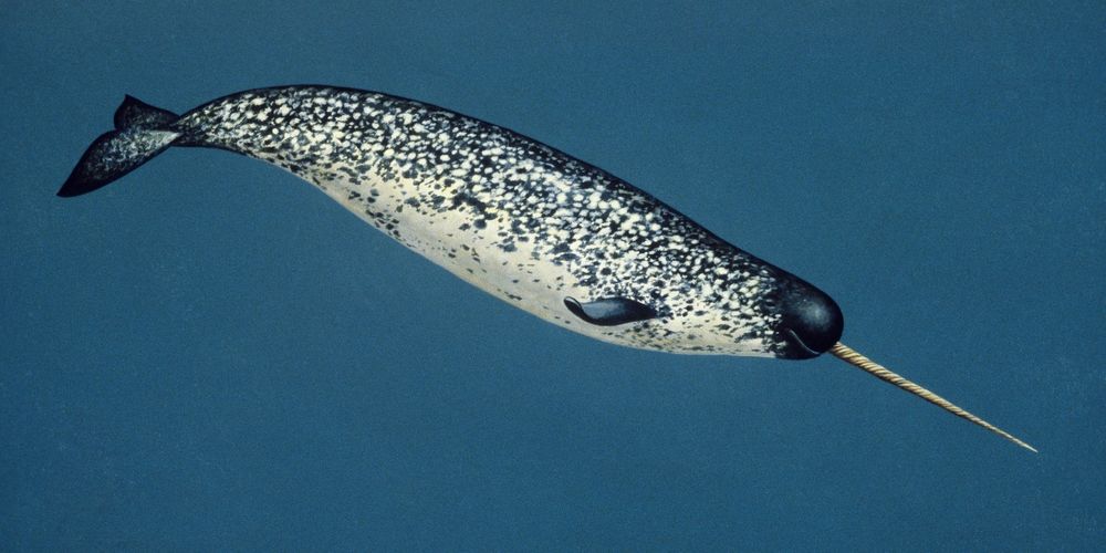 | 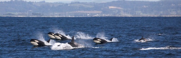 |
| Figure 12: Narwhal (left) and killer whales (right). |
Generally, impacts of climate change on Earth’s ecosystems will be larger for high emission scenarios and smaller for low emission scenarios. Earth’s ecosystems are resilient. They have experienced large climate changes in the past, such as during the ice age cycles of the Pleistocene. However, current rates of change and those expected for the future are larger for some climate variables than past rates (Fig. 13), which has many scientists concerned about the adaptability of ecosystems.
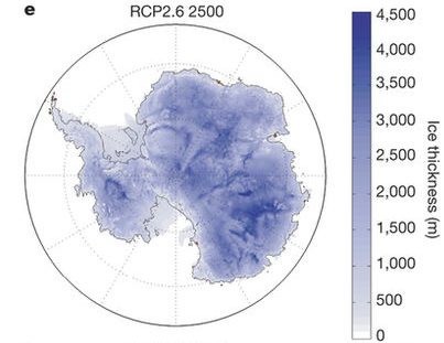
Due to the long lifetime of carbon in the Earth system current human activities will affect many future generations. The ultimate fate of anthropogenic carbon is burial in ocean sediments. This is a slow process that takes tens of thousands of years to remove all of the extra carbon. For this reason much of the carbon we’re putting into the atmosphere today will impact climate and Earth’s physical, biological and human systems for a long time. The total amount of available fossil fuels still in the ground is uncertain (~10,000 PgC, GEA, 2012), but it is clear that enough exists to melt all major ice sheets, which would raise sea level by about 65 m. Fig. 13 shows scenarios of up to about 5,000 GtC, which leads to complete melting of the Greenland and West Antarctic ice sheets and most of the East Antarctic ice sheet with a sea level rise of about 50 m. Even the relatively low (1,280 GtC) emission scenario would lead to a long term sea level rise of about 25 m. However, the rate of change would be much slower for the lower emission scenario (0.5 m/century) compared with the higher scenario (3 m/century). Such rates are unprecedented in more than 8,000 years. High emission scenarios would melt essentially all mountain glaciers on Earth, whereas low emission scenarios would melt about 70% of current glaciers, mostly within this and the next century (Marzeion et al., 2012). Global warming for all but the low emission scenarios will be similar to or even exceed that from the Last Glacial Maximum to the early Holocene (~4ºC). Transformations of Earth’s ecosystems similar in magnitude to those documented for the last deglaciation can therefore be expected for intermediate and high emission scenarios. Because of the prominence of the human influence the period since the industrial revolution has been called the Anthropocene.
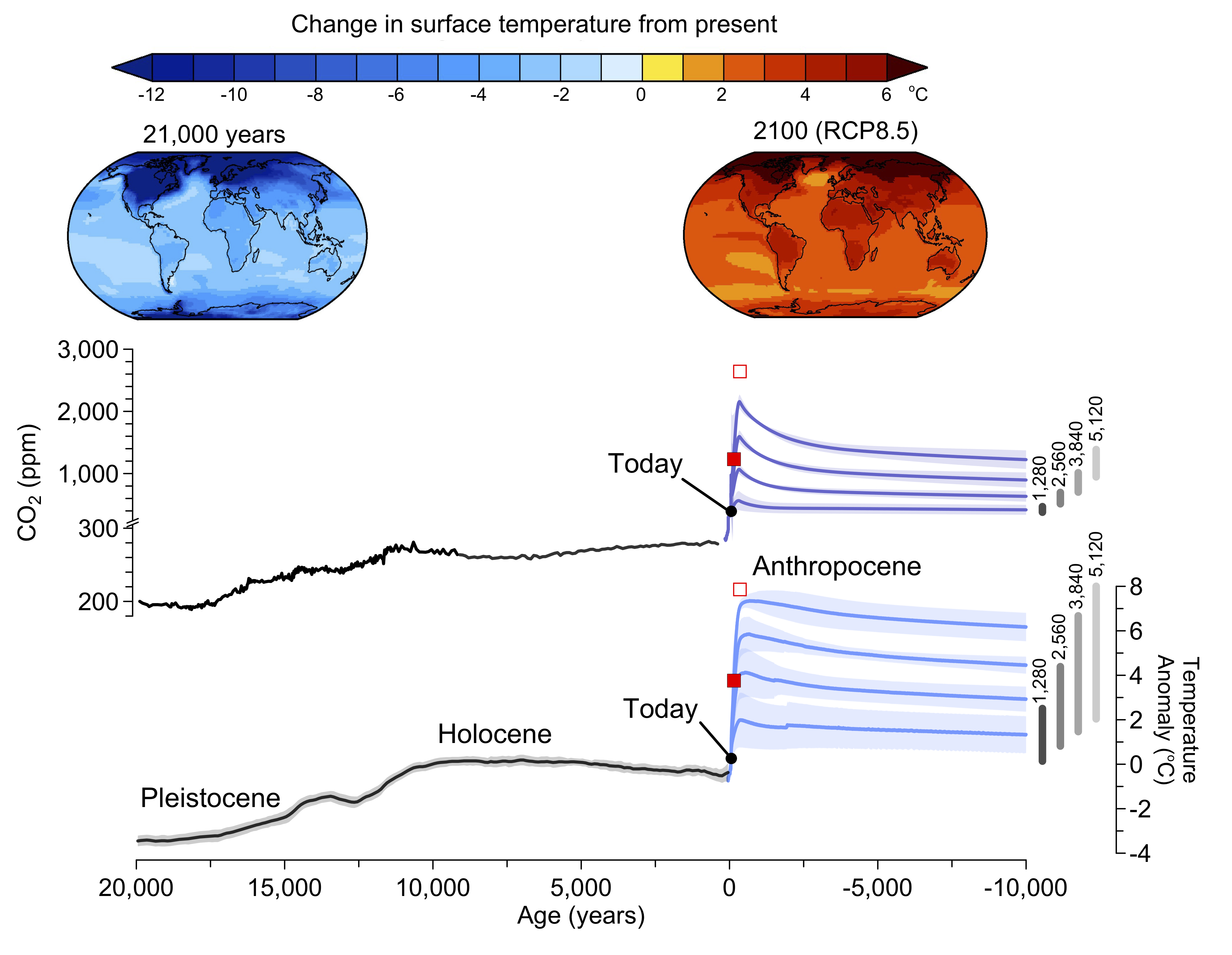 |
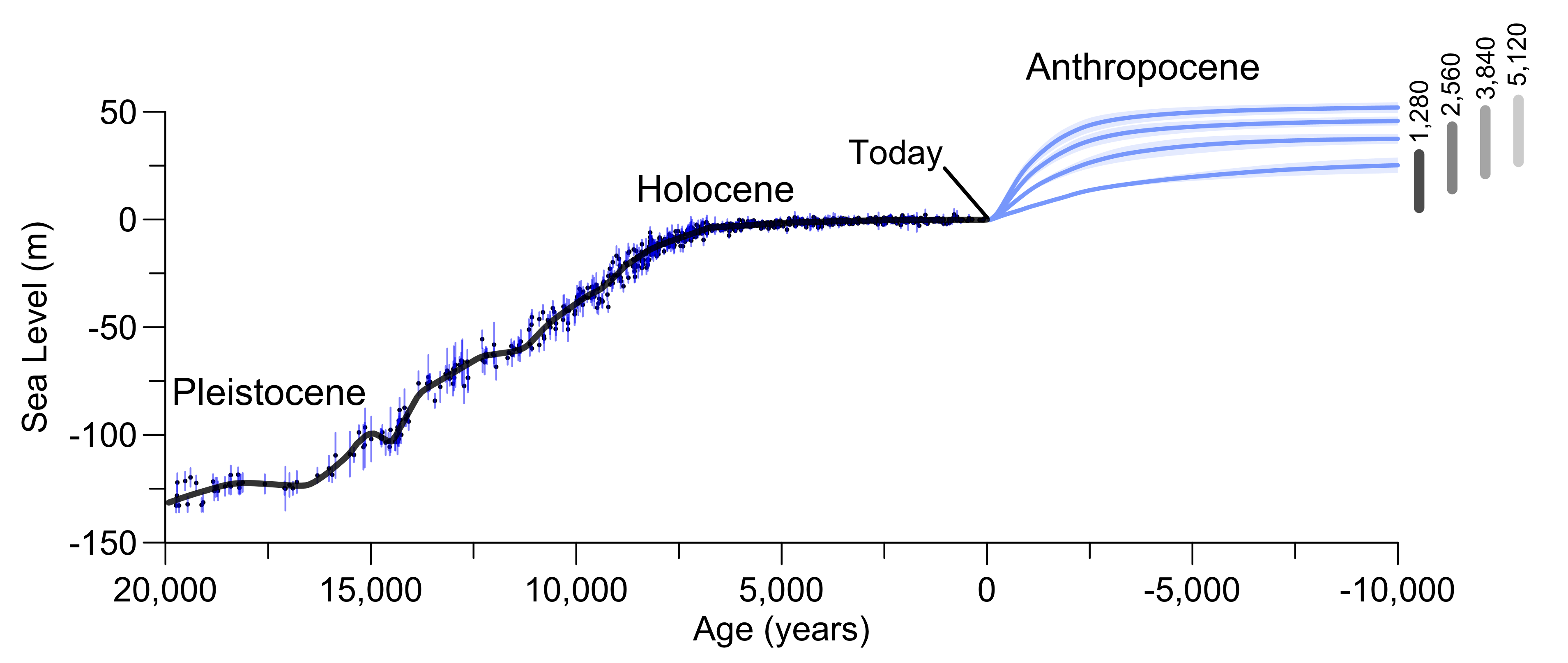 Figure 13: Long-term projected future in the perspective of past changes in atmospheric CO2, surface temperature and sea level. Top: maps show model simulated temperature anomalies (with respect to the preindustrial) for the Last Glacial Maximum (21,000 years ago at the end of the Pleistocene) and projections for the year 2100 based on the RCP8.5 emission scenario. Center and bottom: changes in CO2, global surface temperature and sea level from paleo data and model projections. Intermediate complexity models were used for the future projections assuming a total of 1,280, 2,560, 3840, and 5,120 PgC emissions shown in the blue lines with shading indicating uncertainty. Red squares indicate results from years 2100 (solid) and 2300 (open) for the RCP8.5 scenario for comparison. Vertical gray bars show the range of uncertainty based on a range for climate sensitivity from 1.5 to 4.5ºC. Modified from Clark et al. (2016). Figure courtesy of Shaun Marcott and Peter Clark. |
Sea level rise will have tremendous effects on people living in coastal regions. Clark et al. (2016) estimate that their low emission scenario (1,280 PgC) would submerge an area where currently 1.3 billion people live (19% of the global population) including 25 megacities such as Calcutta, New York, Tokyo, Shanghai, and Cairo. Due to the time lag associated with sea level rise we are already committed to future sea level rise from past emissions. By the year 2000, e.g. humans had emitted ~470 PgC and were committed to a sea level rise of about 2 m. Releasing another 470 PgC would commit us to another 9 m of long-term sea level rise.
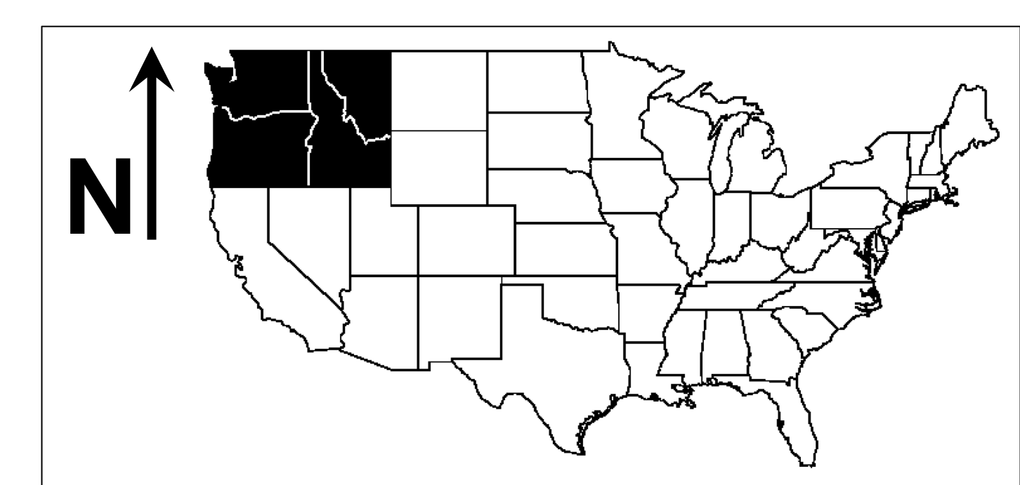
Projected climate impacts vary strongly depending on the region. Small islands and coastal regions will be affected by sea level rise. Polar and alpine regions will be affected by snow and ice loss. Dry regions such as the subtropics will get drier. Detailed regional projections exist for some regions such as North America and Europe. A good resource for regional impacts is part B of this IPCC (2014) report. Here we will only look at one example, which is the western United States of America. Fig. 13 shows that the snowpack there has decreased dramatically during the past 60 years. On average the April 1st snowpack has declined by 15-30% or 25-30 km3, which is similar in volume to the region’s largest man-made reservoir, Lake Mead. Further decreases in snowpack in this region can be expected due to continued warming with impacts on summer stream flows, agriculture and other human water use downstream.
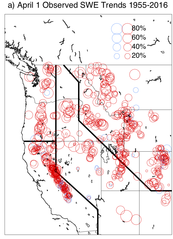
Figure 13: Linear trends in April 1
st Snow Water Equivalent (SWE) observed for the period 1955-2016. Red circles indicate decreased snowpack, blue increased. From
Mote et al. (2018).
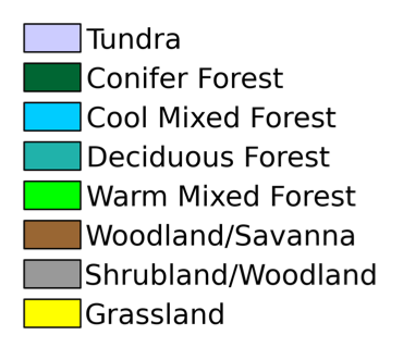
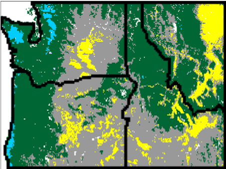
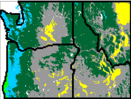
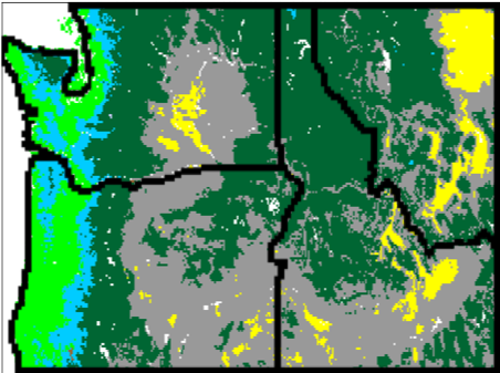
Fig. (14) illustrates that vegetation west of the Cascades mountain range in Oregon and Washington is projected to shift from conifer to more drought-tolerant mixed forest, whereas some of the grassland that occupies the eastern portions of those states as well as parts of Idaho and Montana is projected to be replaced by shrubs and conifer forest. Fires are projected to increase in frequency from 37 to 9 years on average in the full region. Modeled fires for the past are infrequent west of the Cascades (~80 year recurrence time on average), but they are projected to become much more common for high emission scenarios (~27 year recurrence time for RCP8.5) due to warmer and dryer summers. Intermediate emission scenarios lead to less dramatic changes in fire and vegetation.
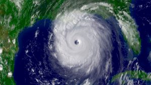
Figure 15: Satellite Image of Hurricane Katrina.
A warming climate implies a shift in the probability distribution such that hot extremes become more frequent and cold extremes become less frequent. This is what is currently observed and we can expect this trend to continue into the future. Due to the intensification of the hydrological cycle we can also expect more droughts and more floods. Changes in other extreme events are less well understood. Occurrences of total hurricanes and typhoons (tropical cyclones) are projected to decrease but the strongest hurricanes are projected to become more frequent (Knutson et al., 2010). This is a concern because those are the ones that inflict the most damage. Hurricane development depends on warm ocean water as an energy source. Latent heat release is also an important fuel for hurricanes and other storms. Thus warmer sea surface temperatures and more latent heat release due to more water vapor in the warmer air will strengthen hurricanes, consistent with observations of increases in the destructiveness of tropical storms in the past decades (Emanuel, 2005). Another important factor for hurricane development, particularly in its early stages, is wind shear. That is how fast winds increase with elevation. Storms require low shear to develop into a coherent vortex, which may become less likely in the future. The end result of changes in wind shear and changes in temperatures is that in a warmer climate the total number of hurricanes will decrease, but strong hurricanes will become more frequent and they will cause more rainfall.
Climate change is already affecting people and more changes can be expected for the future. The decline of sea ice in the Arctic, for example, already affects native people there such as the Inuit. Their life depends on sea ice for hunting and travel and will be greatly affected by the expected future sea ice loss (Watt-Cloutier, 2015; watch her talk here). Sea ice also dampens waves and their effect on erosion of shorelines. Some villages are already threatened by increased erosion due to sea ice loss. On the other hand, a seasonally ice free Arctic will allow for ships to take a shortcut through the Northwest Passage and reduce travel time between the North Atlantic and North Pacific.
Similarly, some mining companies are already planning operations in Greenland in areas that were previously inaccessible due to ice cover. But this opportunity for resource extraction comes of course at the price of sea level rise, which will affect millions of people who live close to shore. Many people will also be affected by the loss of mountain glaciers and their summer water supply. Many current ski areas may no longer be viable in the future due to less snow cover and a shorter season, which will result in job losses there.
Climate change can also lead to conflict. The ongoing civil war in Syria, for example, has been partly caused by a drought, which has been attributed to anthropogenic climate change (Kelley et al., 2015). This attribution is in line with climate model projections that indicate dryer conditions around the Mediterranean in a warmer world (Fig. 6) and paleoclimate data (Cook et al., 2016). Violent conflict about freshwater resources is not new in the history of this and other regions but the current conflict may be the first that is partly caused by anthropogenic climate change. The resulting migrants, many of which fled to central Europe, may be one of the first climate refugees. Conflict and climate refugees may be also be expected from people displaced by sea level rise, such as in Bangladesh or low laying islands. Sea level rise affects people not only through flooding but also by saltwater seeping into the freshwater lens that exists below the ground and provides islanders often with the only source of freshwater. This can also be a problem in other coastal regions.
Questions
- What is the difference between prediction and projection?
- List two uncertainties in climate projections.
- Which tool do climate scientists use for climate projections?
- Are climate models perfect?
- Describe scenarios RCP2.6 and RCP8.5 in terms of carbon emissions and climate change. For which scenario will the impacts be greater?
- How does the global average surface temperature change projected for the end of the 22nd century compare with that between the Last Glacial Maximum and the preindustrial?
- Is projected surface temperature change larger on land or on the ocean? What are the reasons for these differences?
- Where is projected surface temperature change larger, in the tropics or at the poles? What are the reasons for these differences?
- Where are atmospheric temperatures projected to increase most in the tropics? At the surface or at high elevations? What is the reason for this?
- Where is precipitation projected to increase, where to decrease?
- How is evaporation projected to change?
- How is Arctic sea ice projected to change?
- List five different possible impacts of future climate change.
- How much carbon have humans emitted so far, cumulatively?
- How much carbon can we emit in the future if we want to stay below 2ºC above preindustrial global mean temperature?
- What is a tipping point?
- Which ice sheet is closer to a tipping point, Greenland or East Antarctica?
- Why is the West Antarctic ice sheet vulnerable to a warming climate?
- How is the tundra ecosystem projected to change in the future?
- What will be some of the long-term global impacts of past and future anthropogenic carbon emissions?
- What will be some of the regional impacts in the Pacific Northwest?
- How would you expect the frequency of heat waves and cold spells change in the future?
- How are hurricanes expected to change?
- How do you expect future climate change to impacts humans?
Explore Impacts
Explore regional impacts of possible future climate change using this websites:
Lecture: Projections
Lecture: Impacts
Lecture: Tipping Points
Abatzoglou, J. T., and A. P. Williams (2016), Impact of anthropogenic climate change on wildfire across western US forests, Proceedings of the National Academy of Sciences, 113(42), 11770. doi: 10.1073/pnas.1607171113.
Bakker, P., A. Schmittner, J. T. M. Lenaerts, A. Abe-Ouchi, D. Bi, M. R. van den Broeke, W. L. Chan, A. Hu, R. L. Beadling, S. J. Marsland, S. H. Mernild, O. A. Saenko, D. Swingedouw, A. Sullivan, and J. Yin (2016), Fate of the Atlantic Meridional Overturning Circulation: Strong decline under continued warming and Greenland melting, Geophys Res Lett, 43(23), 12,252-212,260, doi: 10.1002/2016GL070457.
Clark, P. U., J. D. Shakun, S. A. Marcott, A. C. Mix, M. Eby, S. Kulp, A. Levermann, G. A. Milne, P. L. Pfister, B. D. Santer, D. P. Schrag, S. Solomon, T. F. Stocker, B. H. Strauss, A. J. Weaver, R. Winkelmann, D. Archer, E. Bard, A. Goldner, K. Lambeck, R. T. Pierrehumbert, and G.-K. Plattner (2016), Consequences of twenty-first-century policy for multi-millennial climate and sea-level change, Nature Clim. Change, 6, 360-369, doi: 10.1038/nclimate2923.
Collins, M., R. Knutti, J. Arblaster, J.-L. Dufresne, T. Fichefet, P. Friedlingstein, X. Gao, W.J. Gutowski, T. Johns, G. Krinner, M. Shongwe, C. Tebaldi, A.J. Weaver and M. Wehner, 2013: Long-term Climate Change: Projections, Commitments and Irreversibility. In: Climate Change 2013: The Physical Science Basis. Contribution of Working Group I to the Fifth Assessment Report of the Intergovernmental Panel on Climate Change [Stocker, T.F., D. Qin, G.-K. Plattner, M. Tignor, S.K. Allen, J. Boschung, A. Nauels, Y. Xia, V. Bex and P.M. Midgley (eds.)]. Cambridge University Press, Cambridge, United Kingdom and New York, NY, USA. pdf
Cook, B. I., K. J. Anchukaitis, R. Touchan, D. M. Meko, and E. R. Cook (2016), Spatiotemporal drought variability in the Mediterranean over the last 900 years, Journal of Geophysical Research: Atmospheres, 121(5), 2060-2074, doi: 10.1002/2015JD023929.
DeConto, R. M., and D. Pollard (2016), Contribution of Antarctica to past and future sea-level rise, Nature, 531(7596), 591-597, doi: 10.1038/nature17145.
Dutkiewicz, S., J. J. Morris, M. J. Follows, J. Scott, O. Levitan, S. T. Dyhrman, and I. Berman-Frank (2015), Impact of ocean acidification on the structure of future phytoplankton communities, Nature Climate Change, 5, 1002, doi: 10.1038/nclimate2722.
Emanuel, K. (2005), Increasing destructiveness of tropical cyclones over the past 30 years, Nature, 436(7051), 686-688, doi: 10.1038/nature03906.
GEA (2012) Global Energy Assessment – Toward a Sustainable Future, Cambridge University Press, Cambridge, UK and New York, NY, USA and the International Institute for Applied Systems Analysis, Laxenburg, Austria. link
Gonzalez, P., R. P. Neilson, J. M. Lenihan, and R. J. Drapek (2010), Global patterns in the vulnerability of ecosystems to vegetation shifts due to climate change, Global Ecology and Biogeography, 19(6), 755-768, doi: 10.1111/j.1466-8238.2010.00558.x.
IPCC (2014) Climate Change 2014: Impacts, Adaptation, and Vulnerability. Part B: Regional Aspects. Contribution of Working Group II to the Fifth Assessment Report of the Intergovernmental Panel on Climate Change [Barros, V.R., C.B. Field, D.J. Dokken, M.D. Mastrandrea, K.J. Mach, T.E. Bilir, M. Chatterjee, K.L. Ebi, Y.O. Estrada, R.C. Genova, B. Girma, E.S. Kissel, A.N. Levy, S. MacCracken, P.R. Mastrandrea, and L.L. White (eds.)]. Cambridge University Press, Cambridge, United Kingdom and New York, NY, USA, pp. 688. link
Kelley, C. P., S. Mohtadi, M. A. Cane, R. Seager, and Y. Kushnir (2015), Climate change in the Fertile Crescent and implications of the recent Syrian drought, Proceedings of the National Academy of Sciences, 112(11), 3241. link
Knutson, T. R., J. L. McBride, J. Chan, K. Emanuel, G. Holland, C. Landsea, I. Held, J. P. Kossin, A. K. Srivastava, and M. Sugi (2010), Tropical cyclones and climate change, Nat Geosci, 3, 157, doi: 10.1038/ngeo779.
Larsen, J.N., O.A. Anisimov, A. Constable, A.B. Hollowed, N. Maynard, P. Prestrud, T.D. Prowse, and J.M.R. Stone, 2014: Polar regions. In: Climate Change 2014: Impacts, Adaptation, and Vulnerability. Part B: Regional Aspects. Contribution of Working Group II to the Fifth Assessment Report of the Intergovernmental Panel on Climate Change [Barros, V.R., C.B. Field, D.J. Dokken, M.D. Mastrandrea, K.J. Mach, T.E. Bilir, M. Chatterjee, K.L. Ebi, Y.O. Estrada, R.C. Genova, B. Girma, E.S. Kissel, A.N. Levy, S. MacCracken, P.R. Mastrandrea, and L.L. White (eds.)]. Cambridge University Press, Cambridge, United Kingdom and New York, NY, USA, pp. 1567-1612. link
Manabe, S., and R. F. Strickler (1964), Thermal Equilibrium of the Atmosphere with a Convective Adjustment, J. Atmos. Sci., 21, 361-385. pdf
Marzeion, B., A. H. Jarosch, and M. Hofer (2012), Past and future sea-level change from the surface mass balance of glaciers, The Cryosphere, 6(6), 1295-1322, doi: 10.5194/tc-6-1295-2012.
Matthews, H. D., N. P. Gillett, P. A. Stott, and K. Zickfeld (2009), The proportionality of global warming to cumulative carbon emissions, Nature, 459(7248), 829-U823, doi: 10.1038/Nature08047.
Moritz, M. A., M.-A. Parisien, E. Batllori, M. A. Krawchuk, J. Van Dorn, D. J. Ganz, and K. Hayhoe (2012), Climate change and disruptions to global fire activity, Ecosphere, 3(6), 1-22, doi: 10.1890/ES11-00345.1.
Mote, P. W., S. Li, D. P. Lettenmaier, M. Xiao, and R. Engel (2018), Dramatic declines in snowpack in the western US, npj Climate and Atmospheric Science, 1(1), 2, doi: 10.1038/s41612-018-0012-1.
Robinson, A., R. Calov, and A. Ganopolski (2012), Multistability and critical thresholds of the Greenland ice sheet, Nature Climate Change, 2, 429, doi: 10.1038/nclimate1449.
Sheehan, T., D. Bachelet, and K. Ferschweiler (2015), Projected major fire and vegetation changes in the Pacific Northwest of the conterminous United States under selected CMIP5 climate futures, Ecological Modelling, 317, 16-29, doi: 10.1016/j.ecolmodel.2015.08.023.
Stocker, T.F., D. Qin, G.-K. Plattner, L.V. Alexander, S.K. Allen, N.L. Bindoff, F.-M. Bréon, J.A. Church, U. Cubasch, S. Emori, P. Forster, P. Friedlingstein, N. Gillett, J.M. Gregory, D.L. Hartmann, E. Jansen, B. Kirtman, R. Knutti, K. Krishna Kumar, P. Lemke, J. Marotzke, V. Masson-Delmotte, G.A. Meehl, I.I. Mokhov, S. Piao, V. Ramaswamy, D. Randall, M. Rhein, M. Rojas, C. Sabine, D. Shindell, L.D. Talley, D.G. Vaughan and S.-P. Xie, 2013: Technical Summary. In: Climate Change 2013: The Physical Science Basis. Contribution of Working Group I to the Fifth Assessment Report of the Intergovernmental Panel on Climate Change [Stocker, T.F., D. Qin, G.-K. Plattner, M. Tignor, S.K. Allen, J. Boschung, A. Nauels, Y. Xia, V. Bex and P.M. Midgley (eds.)]. Cambridge University Press, Cambridge, United Kingdom and New York, NY, USA. link
Watt-Cloutier, S. (2015) The Right to Be Cold, Penguin Canada Books, Ontario, Toronto. link youtube
Weertman, J. (1961) Stability of Ice-Age Ice Sheets, J. Geophys. Res. 66 (11), 3783-3792, doi: 10.1029/JZ066i011p03783.


 . Some are a little faster, others are a little slower. Only the fastest will be able to leave the water phase and make it to the vapor phase (air). (
 , where R = 18O/16O is the heavy over light ratio of a sample, relative to that of a standard Rstd. Fig. B2 illustrates how fractionation during evaporation and condensation affects the isotope values of water, vapor, and ice in the global hydrological cycle.
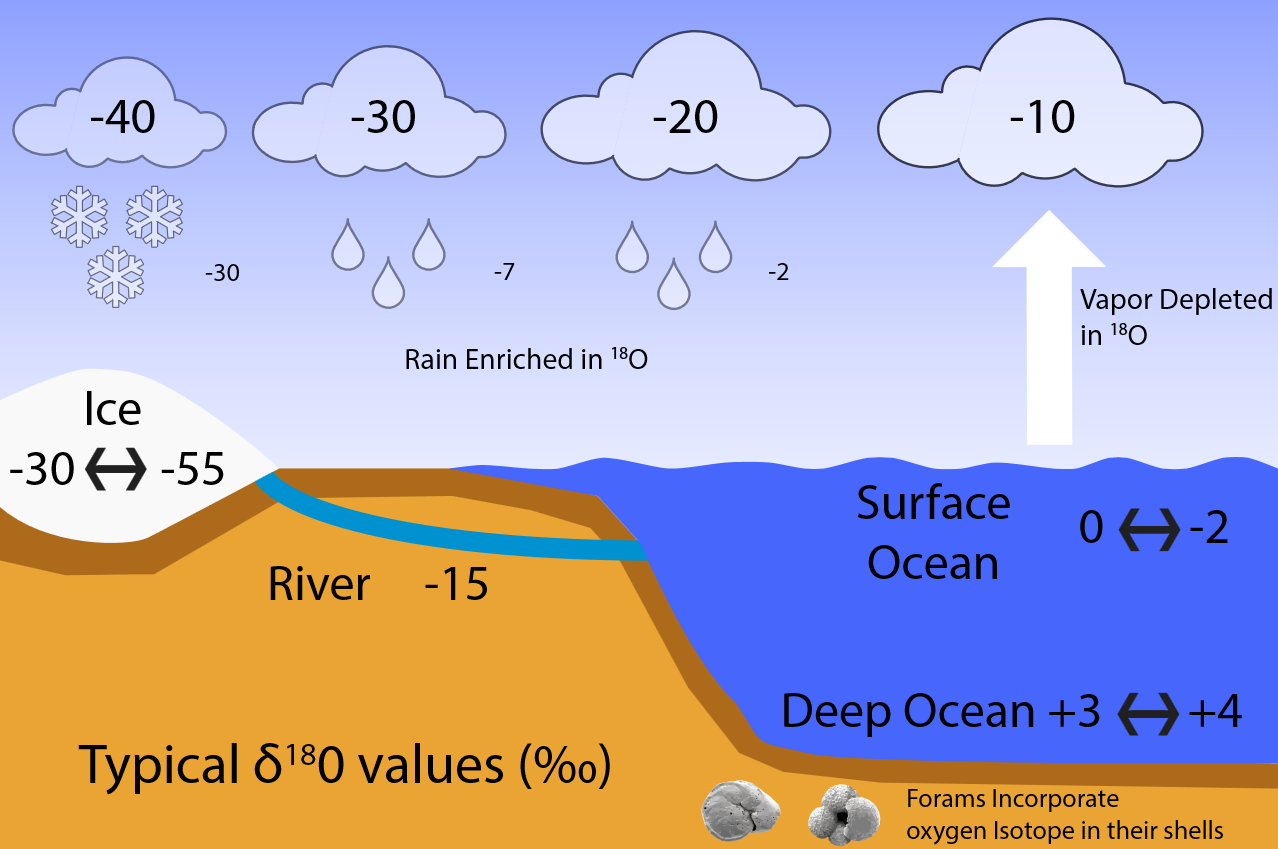
![Glacial-interglacial Cycles. Top: Antarctic temperature anomaly estimated from deuterium ratios measured in the ice (Jouzel et al., 2007). Deuterium (D) is the heavy hydrogen isotope 2H. In H2O it works similar to the heavy oxygen isotope as a local temperature proxy. Center: Atmospheric CO2 concentrations from ice cores (Lüthi et al., 2008). Bottom: Global sea level changes (ΔSL = [δ18O - 3.2 ‰]×[-120 m / 1.69 ‰]) estimated from oxygen isotopes (δ18O) measured in benthic foraminifera from deep-sea sediments (Lisiecki and Raymo, 2004). This is a key figure.](https://open.oregonstate.education/app/uploads/sites/37/2019/07/f10_co2_temp_d18o_t3-1024x735.png)


 of its molecules. The faster they move the higher the temperature. At absolute zero temperature T = 0 K all motions would cease.
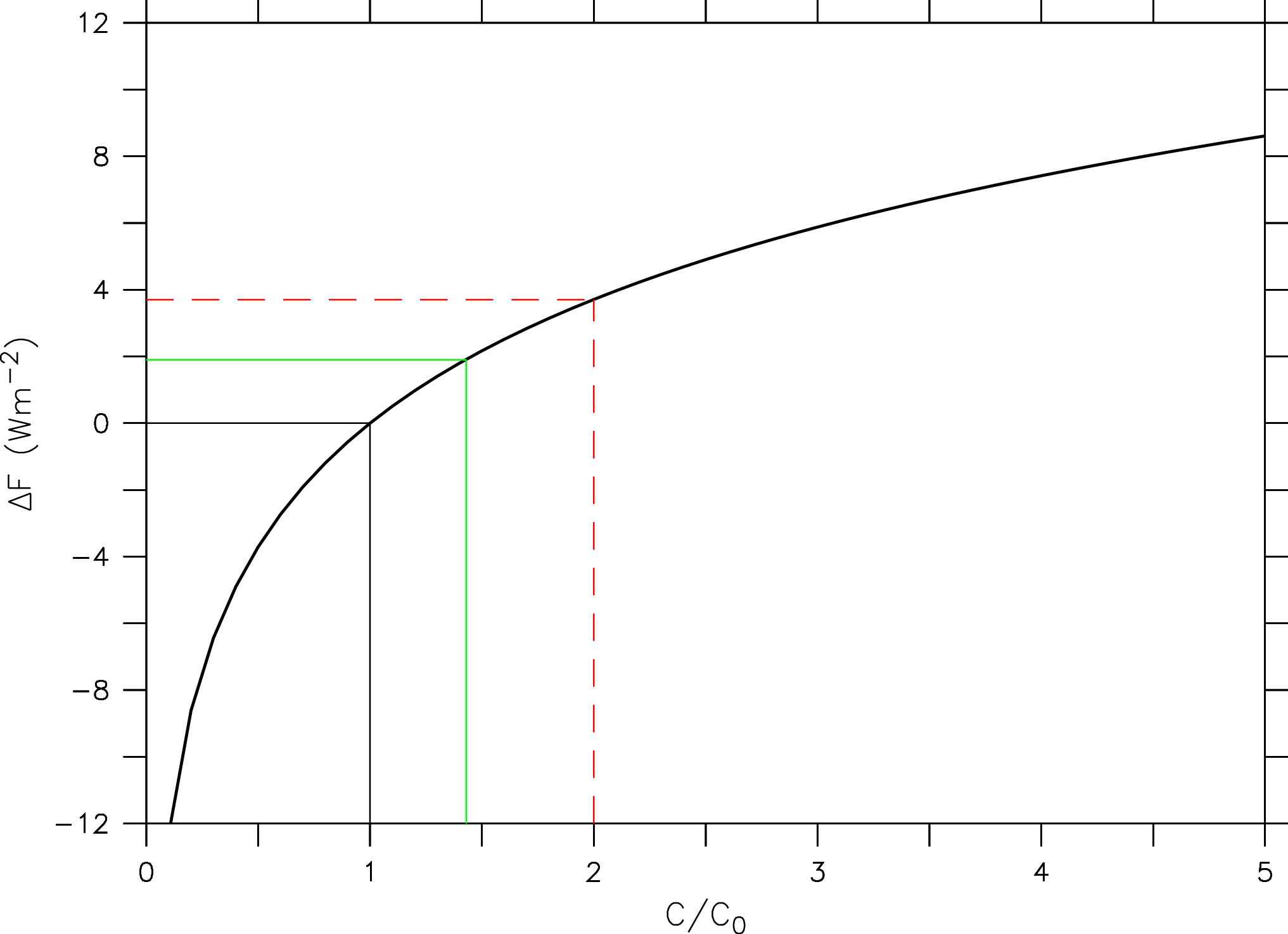
![\begin{equation*} \Delta F = 5.35 [\mathrm{Wm^{-2}}] \ln (C / C_{0}), \end{equation*}](https://open.oregonstate.education/app/uploads/quicklatex/quicklatex.com-2a2bafa1897664c0bc5791dde075c809_l3.svg "Rendered by QuickLaTeX.com")