Appendix B: Probability
B.0.1 Probability Distributions
Probability Mass Function
A probability mass function for a discrete random variable [latex]k[/latex] is defined such that [latex]P(k)[/latex] is the probability of the variable taking the value [latex]k[/latex]. These distributions are normalized, meaning summing over all possible values will equal [latex]1[/latex]. In other words:
[latex]\sum_k P(k) = 1[/latex]
Probability Density Functions
For continuous random variables [latex]x[/latex], a Probability Density Function gives the value [latex]f(x)[/latex] corresponding to the likelihood of the random variable taking on that value, and probabilities are computed from
[latex]P(a \le x \le b) = \int_a^b f(x)dx[/latex]
Integrating over all values of [latex]x[/latex] will equal [latex]1[/latex].
[latex]\int_{-\infty}^{\infty} f(x)dx = 1[/latex]
B.0.2 Conditional Probability
In probability, we often want to talk about conditional probability, which gives us the probability of an event given that we know that another event has occurred.
[latex]P(A|B) = \frac{P(A \cap B)}{P(B)}[/latex]
Bayes’ Theorem tells us that:
[latex]P(A|B) = \frac{P(B|A)P(A)}{P(B)}[/latex]
We can also expand a probability of an event into the conditional probabilities of each other condition, times the probability of these other events.
[latex]P(x) = \sum_{i=1}^N P(x|A_i)P(A_i)[/latex]
This expression [latex]P(x)[/latex] is often called the evidence. We can express the probability of [latex]A[/latex] given [latex]x[/latex], which is called the posterior probability by
[latex]P(A|x) = \frac{P(x|A)P(A)}{P(x)}[/latex]
Also in this equation, [latex]P(x|A)[/latex] is called the likelihood, and [latex]P(A)[/latex] is called the prior.
B.0.3 Bernouli Distribution
One of the simplest probability distributions we should consider is the Bernoulli Distribution. It is essentially a single event, with a probability of success denoted [latex]p[/latex], and a probability of failure of [latex]q=1-p[/latex].
Example 1: A coin toss. Heads or tails? Typically for a fair coin, this will be such that [latex]p=q=0.5[/latex].
Example 2: Selecting a single nucleotide from the genome at random. Is it purine (A or G) or is it pyrimidine (C or T)? For the human genome, the GC content is about [latex]0.417[/latex], but it varies from chromosome to chromosome.
B.0.4 Binomial Distribution
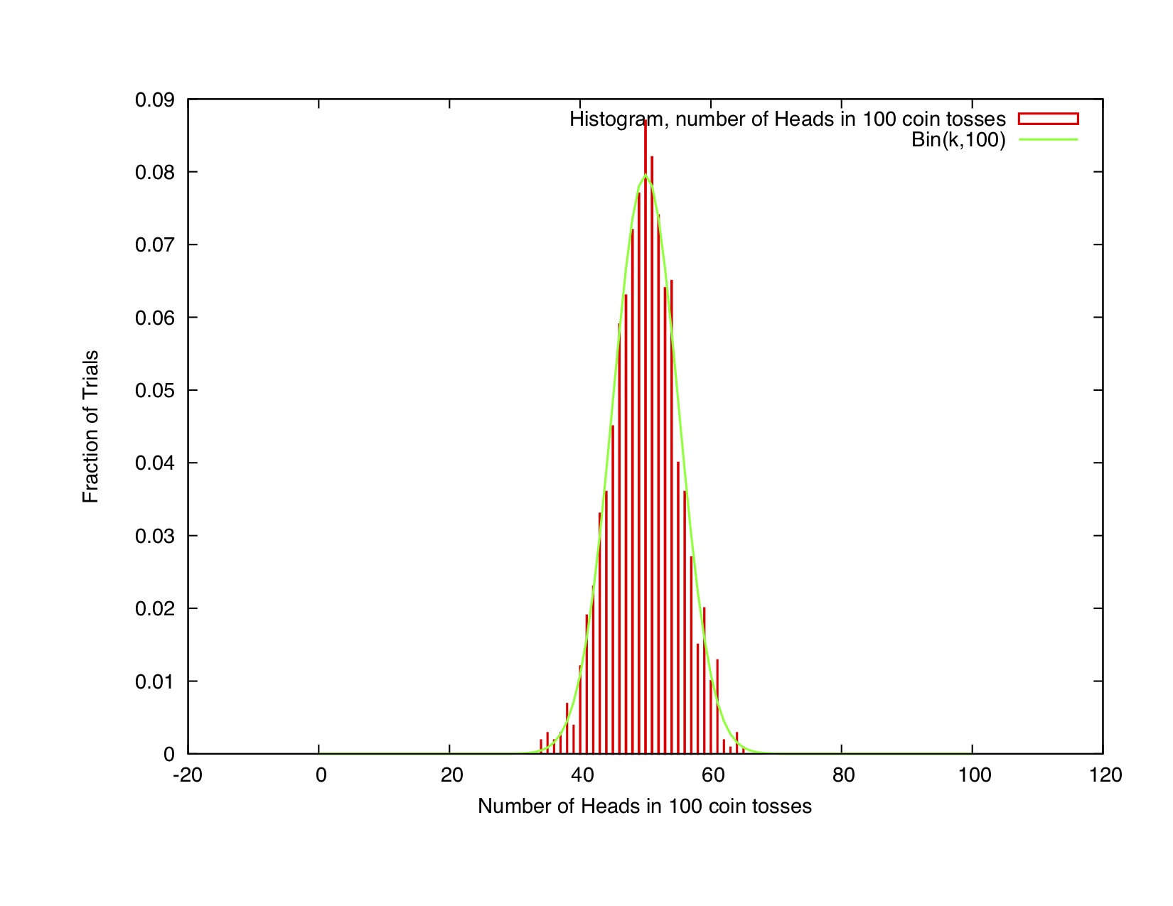
Central to the Binomial distribution is the binomial coefficient [latex]{n \choose k} = \frac{n!}{(n-k)!k!}[/latex] The number of ways to have [latex]k[/latex] successes out of [latex]n[/latex] trials is [latex]{n \choose k}[/latex]. The probability of observing [latex]k[/latex] successes out of [latex]n[/latex] trials is [latex]P(k|p,n) = {n \choose k} p^k q^{n-k}[/latex]. Since [latex]p+q=1[/latex], and [latex]1[/latex] raised to the [latex]n[/latex]th power is still [latex]1[/latex], we can see that these probabilities are normalized (sum to one) by the equation:
[latex]1 = (p+q)^n = \sum_{k=0}^n {n \choose k} p^k q^{n-k}[/latex]
Example 1: Consider tossing a fair coin 100 times, and repeating this for 1000 trials. A histogram for [latex]k[/latex], number of heads in [latex]n[/latex] tosses is shown in Figure B.1. The expected value of [latex]k[/latex] is [latex]E[k] = np[/latex], and the variance is [latex]ar(k) = npq[/latex].
B.0.5 Multinomial Distribution
The multinomial distribution deals which situations when there are more than two possible outcomes (for example, DNA nucleotides). The multinomial coefficient, [latex]M(\vec{n})[/latex], in this example describes the number of ways to have a sequence of length [latex]n[/latex], with the number of occurrences of A,C,G,and T to be [latex]n_A, n_C, n_G,[/latex] and [latex]n_T[/latex] respectively.
[latex]M(\vec{n}) = \frac{n!}{n_A! n_C! n_G! n_T!}[/latex]
The probability of a particular set of observed counts [latex]\vec{n} = (n_A, n_C, n_G,n_T)[/latex] depends on the frequencies [latex]\vec{p} = (p_A, p_C, p_G,p_T)[/latex] by the expression:
[latex]P(\vec{n}|\vec{p}) = \frac{n!}{n_A! n_C! n_G! n_T!} \prod_{i=A}^T p_i^{n_i}[/latex]
B.0.6 Poisson Distribution
The Poisson Distribution describes the number of observed events given an expected number of occurrences [latex]\lambda[/latex]. Consider, for example, the probability of a red car driving past a particular street corner in your neighborhood. The Poisson distribution probability mass function is given by:
[latex]P(k|\lambda) = \frac{\lambda^k e^{-\lambda}}{k!}[/latex]
It has one parameter [latex]\lambda[/latex], which is also the expected value of [latex]k[/latex] and the variance ([latex]E[k] = var(k) = \lambda[/latex]).
It can be shown that for fixed [latex]\lambda = np[/latex], and for [latex]n \rightarrow \infty[/latex], the Binomial distribution is equivalent to the Poisson distribution.
In many applications, the [latex]\lambda[/latex] parameter for the Poisson distribution is treated as a rate. In this case, the expected value of [latex]k[/latex] is [latex]E[k] = \lambda \ell[/latex], so that [latex]\lambda[/latex] describes the rate of occurrence of the event per unit time (or per unit distance, or whatever the application is). The probability distribution is given by:
[latex]P(k,\ell|\lambda) = \frac{(\lambda \ell)^k e^{-\lambda \ell}}{k!}[/latex]
Example: Consider modeling the number of mutations [latex]k[/latex] observed in a length of DNA [latex]\ell[/latex].
Consider the important case when [latex]k=0[/latex] for the Poisson Distribution.
[latex]P(k=0,\ell|\lambda) = e^{-\lambda \ell}[/latex]
The probability that [latex]k[/latex] is not zero, is therefore:
[latex]P(k \leq 0,\ell|\lambda) = 1 - e^{-\lambda \ell}[/latex]
Now consider [latex]\ell[/latex] being replaced by a random variable [latex]x[/latex].
B.0.7 Exponential Distribution
The Exponential distribution is related to the Poisson by equation [latex]B.1[/latex]. It is the probability of an event occurring in a length [latex]x[/latex]. The cumulative distribution function [latex]F(x)[/latex] is the same as this last equation:
[latex]F(x|\lambda) = 1 - e^{- \lambda x}[/latex]
And the probability density function is the derivative of the cumulative distribution function:
[latex]P(x|\lambda) = \lambda e^{- \lambda x}[/latex]
Note that whereas the Poisson distribution is a discrete distribution, the Exponential distribution is continuous and [latex]x[/latex] can take on any real value such that [latex]x \ge 0[/latex].
B.0.8 Normal Distribution
A very important distribution for dealing with data, the normal distribution models many natural processes. We already saw that the binomial distribution looks like the normal distribution for large [latex]n[/latex]. Indeed, the Central Limit Theorem states that the sum of random variables approaches normal distribution for a large [latex]n[/latex]. Here is the probability density function:
[latex]P(x|\mu,\sigma) = \frac{1}{\sqrt{2 \pi \sigma^2}} e^{\frac{-(x - \mu)^2}{2 \sigma^2}}[/latex]
B.0.9 Extreme Value Distribution
The maximum value in a set of random variables [latex]X_1, ... , X_N[/latex] is also a random variable. This variable is described by the Extreme Value Distribution, also known as the Gumbel Distribution.
[latex]F(x|\mu,\sigma,\xi) = \exp \left\{ - \left[ 1+\xi \left( \frac{x - \mu}{\sigma} \right) \right]^{-1/\xi} \right\}[/latex]
For [latex]{1+\xi(x - \mu)/\sigma \gt 0}[/latex], and with a location parameter [latex]\mu[/latex], a location parameter [latex]\sigma[/latex], and a shape parameter [latex]\xi[/latex]. In the limit that [latex]xi \rightarrow 0[/latex], the distribution reduces to:
[latex]F(x|\mu,\sigma) = \exp \left\{ - \exp \left( - \frac{x - \mu}{\sigma} \right) \right\}[/latex]
In many cases, for practical purposes, one makes the assumption that [latex]\xi \rightarrow 0[/latex].
