Prologue
1 The Human Age
It happened, one day about noon going towards my boat, I was exceedingly surprised, with the print of a man’s naked foot on the shore, which was very plain to be seen in the sand. I stood like one thunder-struck, or as if I had seen an apparition . . .
—Daniel Defoe, The Life and Adventures of Robinson Crusoe
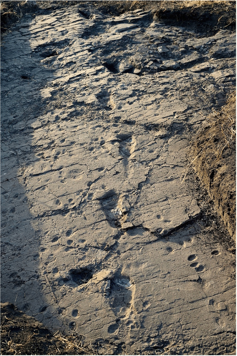
One day about 3.7 million years ago, a group of our close relatives in the genus Australopithecus went for a walk in the open savanna of what would many years later be named Laetoli, Tanzania. A recent rain had turned a deposit of volcanic ash into a sticky runway of mud. Undaunted by the minor obstacle, the group trudged onward, leaving behind what was at the time a rather unremarkable set of footprints.1 The folks who made those footprints were not exactly us, but it is hard to look at their footprints and not feel a deep sense of kinship (Fig. 1.1). Their tracks, along with the dozen or so other fossil hominin footprints that have been found around the world, could quite easily have been humanity’s lasting mark on the planet. It was far from certain that our lineage would persist. Indeed, with the exception of Homo sapiens, all the other members of our hominin family tree have gone extinct. That includes relatives that were seemingly just as skilled and accomplished as us. Homo erectus designed and manufactured sophisticated tools, had complex social interactions, and inhabited myriad different environments across two continents.2 That wasn’t enough to prevent them from going extinct 100,000 years ago and ending an almost 2-million-year run. Similarly, Neanderthals (H. neanderthalensis) made tools, wore clothes, built homes, controlled fire, buried their dead, and even had children with us, none of which prevented their extinction about 40,000 years ago.
We don’t know why we were the sole hominin survivors. Perhaps it was the unique skills that we possessed compared to our relatives.3 But it could also have simply been random luck.4
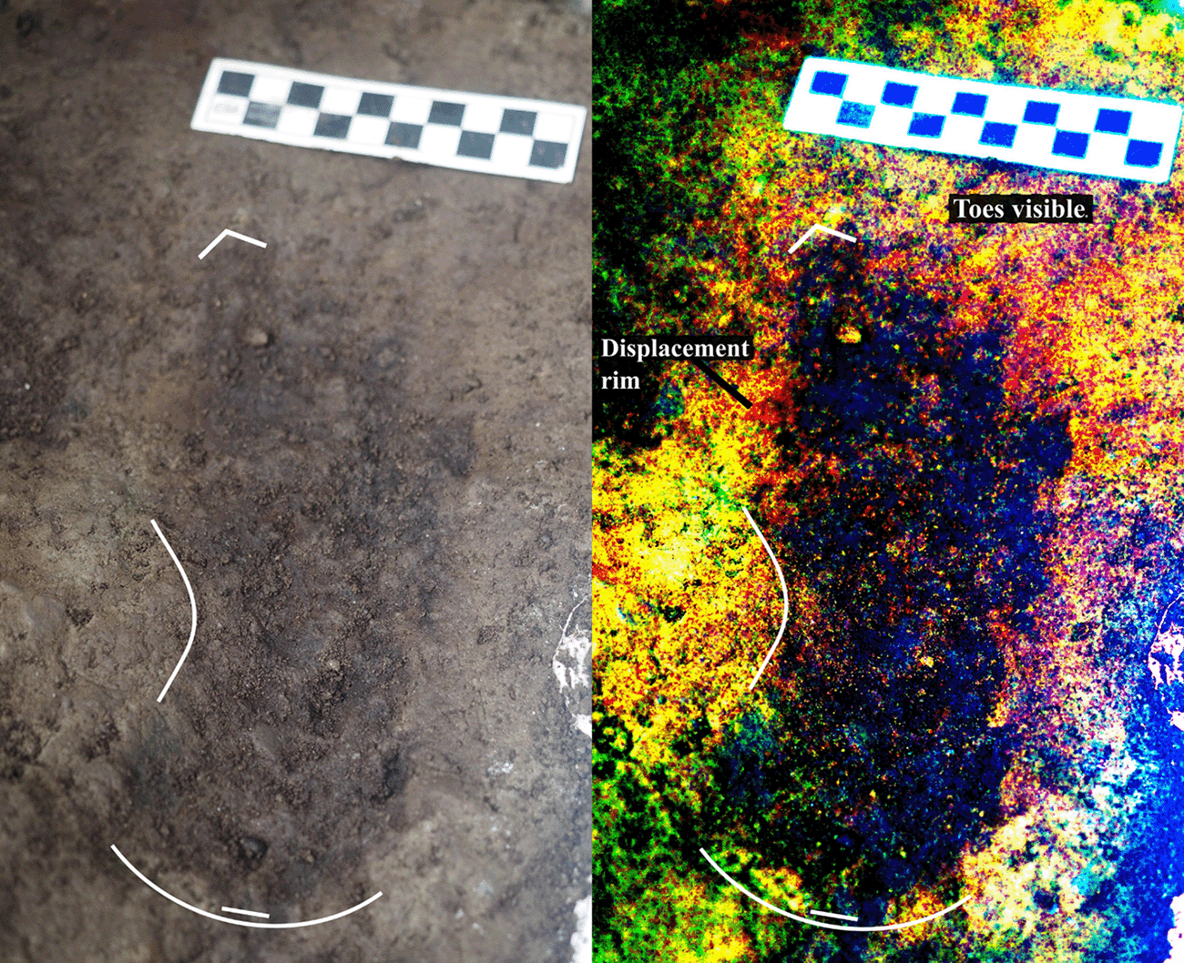
Whatever the reason, we certainly didn’t look back. By the end of the Pleistocene, humans had spread to almost every corner of the planet. We also were beginning to leave more lasting marks than just a few footprints. Early evidence of our growing influence on the planet comes from a group of people that were living along the coastline of British Columbia, Canada, 13,000 years ago. Those people also left behind a few footprints (Fig 1.2), along with prodigious shell mounds that were by-products of their adept skill at exploiting the region’s marine resources. Calcium leaching from the shell mounds slowly increased the pH of the surrounding soil, which in turn increased the availability of phosphorous to plants. That fertilization made the surrounding forest far more productive than it otherwise would be, and the increased productivity persists today.5
It is not clear whether the forest fertilization was deliberate or an accident of unplanned waste disposal. But other evidence indicates that across the planet, our Pleistocene ancestors were beginning to deliberately shape and manage the world around them. There is fairly strong evidence that they deliberately set fires in order to promote plant and animal species they liked to eat,6 and there is suggestive evidence that some of them may have manipulated the plants around them in more direct ways, such as weeding less desirable species and planting preferred ones.7 They also developed deadly efficient hunting techniques.8
That was just the beginning. The pace, sophistication, and magnitude of our manipulation of the planet (both planned and unplanned) has steadily increased over the past 13,000 years. Today, Earth is as much a reflection of us as we are of it. Our influence has become so ubiquitous, measurable, and durable that a group of scientists are now convinced that we have entered a new geologic epoch known as the Anthropocene.9 In this chapter, I catalog some of the evidence that led these scientists to their conclusion, and I explore some of the reasons why humans are having such an inordinate impact on the planet.
1.1 Time Signatures
Section 1.1: Time Signatures
As far as we can tell, Earth is about 4.5 billion years old. A lot has happened over those years. A list of the greatest moments in Earth’s history might include the appearance of cellular life (3.5 billion years ago, or bya), the first diversification of multicellular organisms (541 million years ago, or mya), the first land animals (428 mya), the first flowering plants (136 mya), and the demise of the dinosaurs (65 mya). That list barely scratches the surface of all the wild and amazing things that have happened on our planet. You can probably tell from the list that I am biased toward biology; a chemist or a geomorphologist might come up with a different list. Describing the long history of the planet can quickly become complex, muddled, subjective, and confusing. To avoid such complications, we need a way of organizing events into a standard timeline that places them in context with one another.
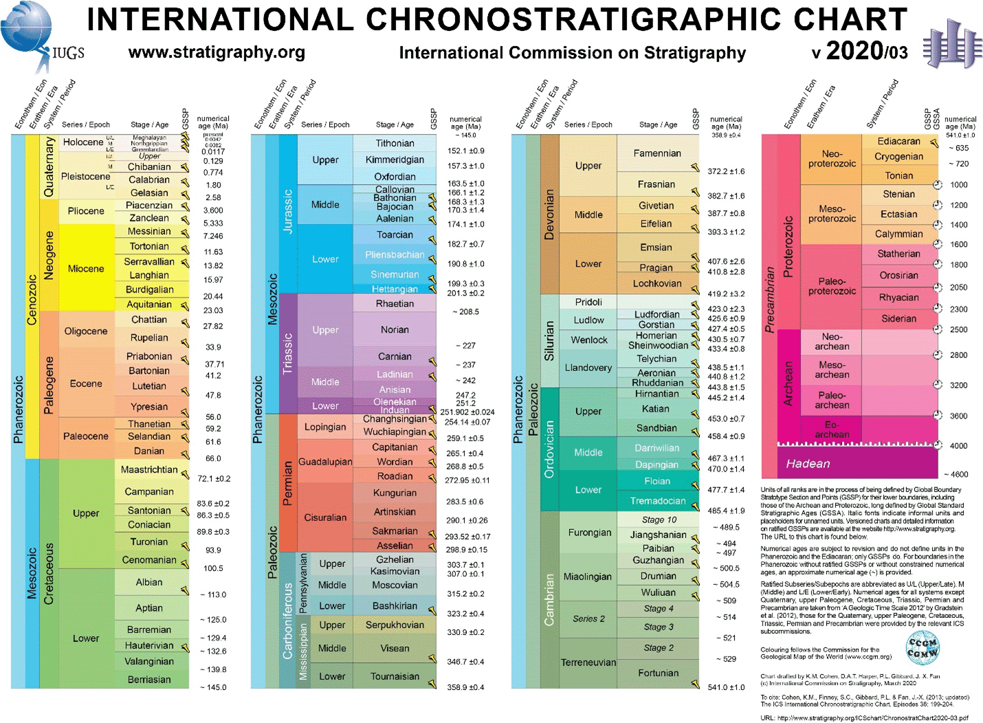
Geologists have come to the rescue. The International Commission on Stratigraphy has developed a standard timeline for the history of Earth that stretches from the formation of the planet to the present day. It is more than just a list of important dates. The International Chronostratigraphic Chart (Fig. 1.3) organizes the history of Earth into a series of nested periods—eons, eras, periods, epochs, and ages—that reflect distinct stages in how the planet looked and felt and what organisms populated it. It somewhat resembles a fancy layer cake, which is no accident: geologists view the world mostly through its rocks. These rocks generally get deposited in progressive layers, with the oldest at the bottom and the youngest at the top. Various geologic processes such as plate tectonics can jumble up that progressive layering a bit, but geologists have gotten good at discerning the original sequence of deposition in complex landscapes. That sequence of rocks as well as the fossils and artifacts contained in them is known as stratigraphy. Much of our understanding of Earth history comes from studying its stratigraphy.
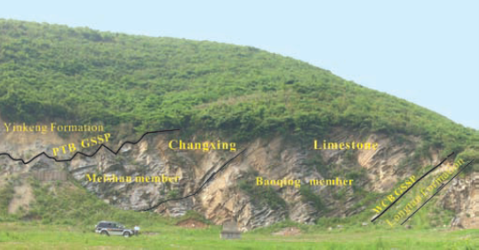
The boundaries that separate the various groupings in the International Chronostratigraphic Chart correspond to an observable shift in stratigraphy. For example, at about 252 mya, something went terribly wrong for most of the species on the planet. It is not clear what exactly happened, but the stratigraphy indicates that during this period, Earth experienced massive volcanic eruptions, was hit by one or more large meteors, and the physical characteristics of its oceans were changing.10 Whatever the exact cause, by the time the dust settled, about 96% of its marine species and about 70% of its terrestrial species had gone extinct. The enormity of this shift is depicted in the International Chronostratigraphic Chart as a transition between two geologic periods (the Permian and Triassic) as well as between two eras (the Paleozoic and Mesozoic). We can see the actual physical changes in stratigraphy that identify the transition at numerous locations around the world, but the International Commission on Stratigraphy thinks the best place to see them is an eroding hillslope near Meishan, China (Fig. 1.4). They have designated the spot as the official example location for the start of the Triassic, the first period of the Mesozoic era.
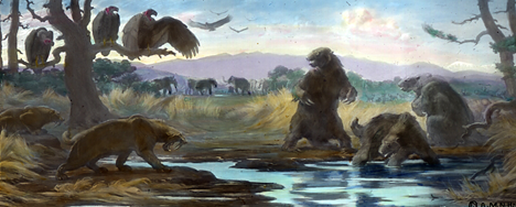
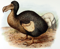
As currently defined by the International Commission on Stratigraphy, we are living in the Holocene epoch, part of the Quaternary period. The Holocene began about 12,000 years ago, when the climate warmed and the latest large-scale retreat of global glaciers began. The shift in climate was also accompanied by a modest (at least at the start) extinction event that was most pronounced among large terrestrial mammals. We know that these changes occurred because of the signatures they left in the stratigraphic record. Analysis of trapped atmosphere in the massive Greenland ice sheet provides a detailed picture of what Earth’s climate was like over the past 123,000 years. This includes warming at the end Pleistocene that is recorded as a shift in concentration of the stable isotopes 2H (deuterium) and 18O. Additionally, at sites around the world, there is a conspicuous loss of large mammals from the fossil record. In North America, 35 genera of mammals went extinct over the span of just a few thousand years.11 While many small- and medium-sized species such as coyotes, skunks, and squirrels survived, a host of oversized megafauna did not (Fig. 1.5).
Like the other shifts in the long stratigraphic record of Earth, we are a bit uncertain about what exactly was driving the shifts in climate and species at the end of the Pleistocene. For unclear reasons, oceans started releasing large amounts of CO2 into the atmosphere toward the end of the Pleistocene, likely triggering the rapid period of warming.12 Climate change is in turn one hypothesis for what caused the extinctions. But the connection is not clear-cut because something else was happening at this time as well: humans were becoming a global species. In many regions, such as North America, extinctions are suspiciously coincident with the first arrival of humans and their increasingly sophisticated hunting skills. The degree to which humans contributed to megafauna extinctions by overhunting is still not well understood, and it is a topic of often heated debate among scientists. It is likely that a combination of factors (including hunting by humans) contributed to the extinctions, and the relative importance of the factors varied across regions.13
The question of what caused extinctions at the end Pleistocene would be a minor academic curiosity if not for the fact that something strange happened as the Holocene epoch progressed. The changes that ushered in the start of the epoch did not stop. In fact, the warming climate and species extinctions have continued to accelerate. In addition, a host of other changes have taken place. The world today looks vastly different than it did 12,000 years ago. Imagine what the Paleolithic fishermen of British Columbia would make of commercial trawlers, aquaculture, logging operations, cattle ranches, freeways, streaming episodes of Twilight, and cities like Vancouver. In contrast to the equivocal evidence that humans helped push megafauna to extinction at the start of the epoch, there is strong evidence that humans have been the main driving force reworking the planet ever since. The accumulating evidence that the world we live in has rapidly changed from the start of the Holocene put the International Commission on Stratigraphy into a bit of a bind. Folks began to ask the obvious question: If the world looks radically different from when the Holocene started, doesn’t that mean we should define a new epoch?
1.2 The Great Acceleration
Section 1.2: The Great Acceleration
Like any good international scientific body, the International Commission on Stratigraphy convened a working group (the Anthropocene Working Group) to study whether a new geologic epoch should be declared. Specifically, the Anthropocene Working Group set out to answer two questions:14
- Have humans changed the Earth System such that geologic deposits forming now and in the recent past include a fingerprint distinct from that of the Holocene Epoch, with high potential to remain in the geological record?
- If so, when did that change become recognizable worldwide?
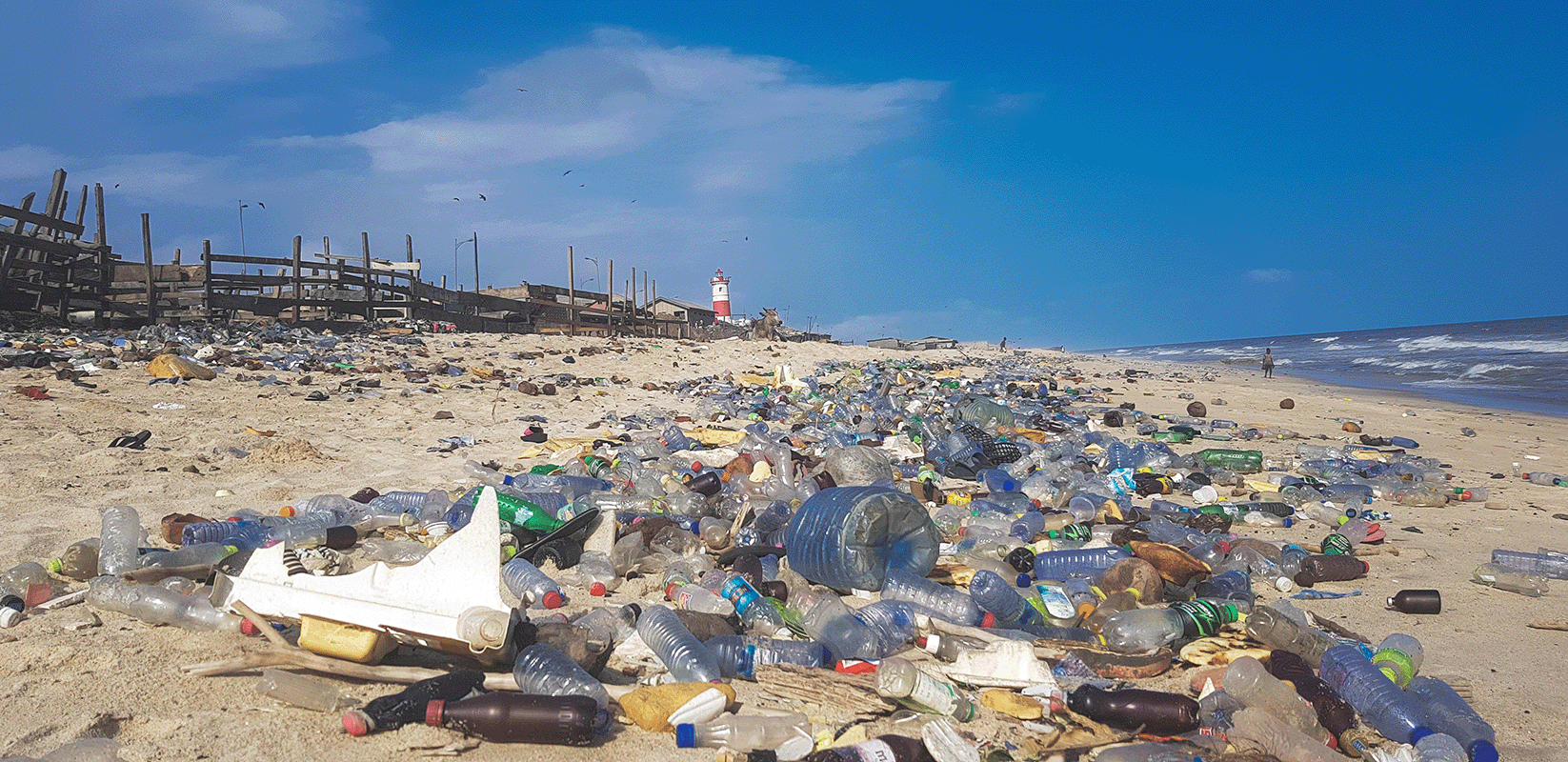
On the first question, the Anthropocene Working Group concluded that there were indeed numerous distinct signatures of humanity that either already have left or were likely to leave a lasting mark in the geologic record (Table 1.1) Our influence is seen in almost all the traits that define our unique planet. We have altered the chemistry of its oceans, changed its climate, reshaped its geomorphology, redesigned its biochemistry, and transformed its biology. Importantly, these changes are global in extent, not just isolated to particular regions. The signatures of humanity have even been found in the most remote and inaccessible parts of the planet. For example, long-lived industrial pollutants such as polychlorinated biphenyls (PCBs), polybrominated diphenyl ethers (PBDEs), and plastics have been found in the tissues of amphipods living in ocean trenches more than 10,000 m deep.15 Remarkably, pollutant levels at the bottom of the trenches rival those of rivers flowing through heavily industrialized regions in China.
| The Stratigraphy of the Anthropocene | ||
|---|---|---|
| Stratigraphic Layer | Signature | Description |
| Layer One | Manufactured materials | These include plastics, ceramics, concrete, black carbon, elemental aluminum, and persistent organic pollutants such as polychlorinated biphenyls (PCB’s). |
| Layer Two | Radiogenic pollution | Fallout from nuclear weapons testing and pollution from other nuclear reactions has left a ubiquitous radiogenic signature across the planet in the form of isotopes such as 14C, 239Pu, and 3H. |
| Layer Three | Altered biogeochemical cycles | Our influence on the C and N cycles is most notable. Combustion of fossil fuels has pushed atmospheric CO2 to levels not seen since the Pliocene Epoch. We have increased the amount of reactive N in the biosphere 120% relative to the Holocene baseline. |
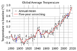
| Layer Four | Altered climate | As of 2020, global average temperature was 1.2°C higher than it was at the start of the industrial revolution; 10 warmest years in the historical record have occurred since 2005 |
| Layer Five | Altered sedimentation | Activities such as agriculture, mineral extraction, and dams have globally altered the creation and transportation of sediment. |
| Layer Six | Changes to the biota | Since the start of the 19th century species extinction rates have spiked above long-term background levels likely driving the Earth toward its 6th mass extinction event within the next few hundred years. |

We can use our understanding of the stratigraphic record to place the current period of Earth System change into historical context. Doing that reveals how unique this period of change is, even in comparison to all the amazing things that have happened over Earth’s 4.5 billion years. Some of the changes are happening for the first time ever, such as the range of new chemical compounds that we invented and made ubiquitous such as PCBs and plastics. In other cases, the type of change is not particularly new but the speed or magnitude of the change is exceptional. We are changing a number of Earth System metrics remarkably quickly compared to the baseline conditions that have existed during most of the Holocene (Table 1.2). That rapid departure from baseline Holocene conditions is a core part of the argument for declaring a new geologic epoch.
| Parameter | Holocene baseline rate of change | Current rate of change | Comparative magnitude |
|---|---|---|---|
| Atmospheric CO2 | -0.17 ppm/century until 7K years ago | 166 ppm/century (1970-2015 average) | 550 times faster than Holocene baseline;10 times faster than during the Paleocene-Eocene Thermal Maximum |
| Global average temperature | -0.01°C/century | 1.7°C/century (1970-2015 average) | 170 faster than the Holocene baseline |
| N cycle | Total nitrogen fixation from natural sources: 203 Tg N/year | Additional nitrogen fixation from human modification: 210 Tg N/year | Reactive nitrogen has doubled compared to the Holocene baseline. Possibly the largest change to the nitrogen cycle in the last 2.5 billion years. |
| P cycle | 10-15 Tg P/yr input to soil (from weathering) | 10-15 Tg P/yr input to soil from enhanced weathering and P mining for fertilizer | 3 times more P released to the environment compared to Holocene baseline |
| Species extinctions | 0.1 extinctions per million species years | 1-10 extinctions per million species years | 10-100 times background rate. |
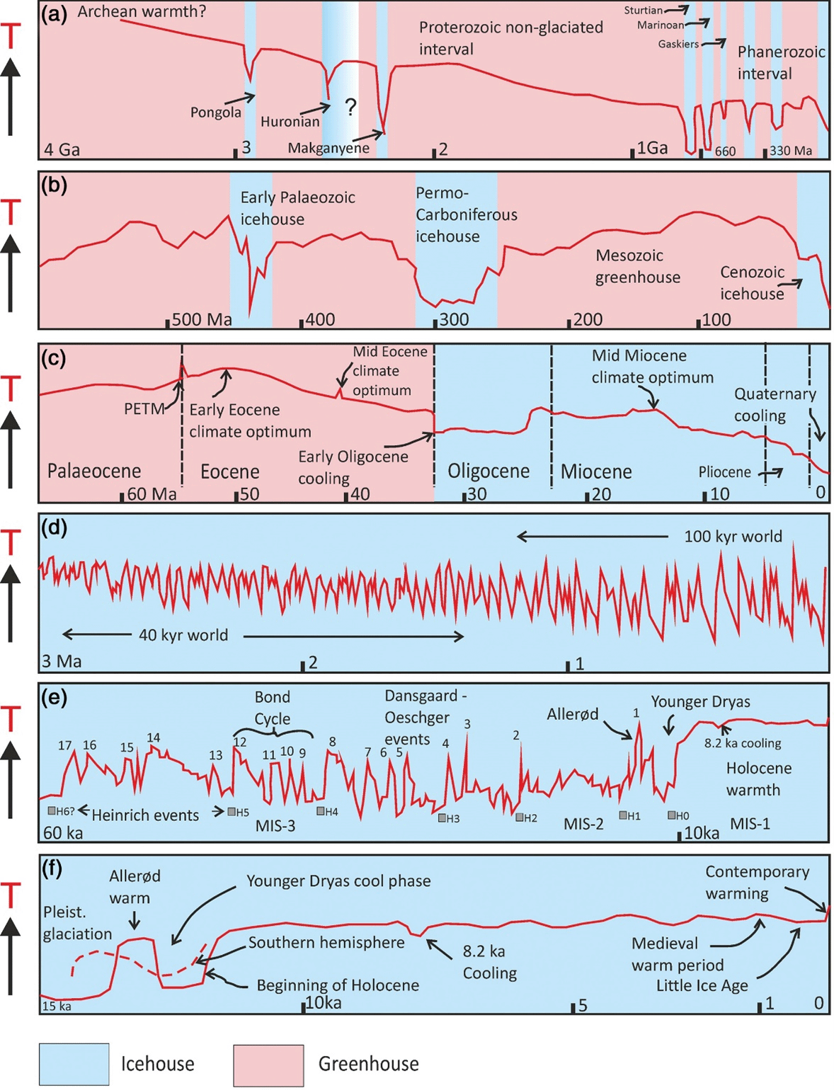
We have compiled relatively good stratigraphic records for some Earth System metrics that go back even further in time. Global climate is one example. Over its history, Earth’s climate has fluctuated between relatively warm greenhouse periods when the poles were ice-free and cooler icehouse periods when large ice sheets dominated the high latitudes. You can see the start of the Anthropocene in Figure 1.6. Look closely; the 1°C warming that has occurred over the past 140 years or so is just a tiny blip at the very end. It can be easy to view that tiny blip as an insignificant hiccup compared to past climate change. That would be wrong. Keep in mind the 4-billion-year timescale of Figure 1.6. On that scale, 140 years is almost impossible to see. The fact that we can nevertheless see a spike in temperature over such a comparatively infinitesimal period is amazing. The stratigraphic record of global temperature records other blips, both up and down. Relative to those, the speed of our current blip is notable. For example, about 55 million years ago, global average temperature rose by about 5°C over a period of just 10,000 years (more or less) during a time known as the Paleocene–Eocene Thermal Maximum (PETM).17 That’s incredibly fast. You can see the spike in Figure 1.6C (see the arrow labeled PETM). The pace of global warming during the PETM was about 0.05°C per century. Since 1880, global average temperature has been increasing at 0.07°C per decade18 —more than 10 times as fast as the spike during the PETM.
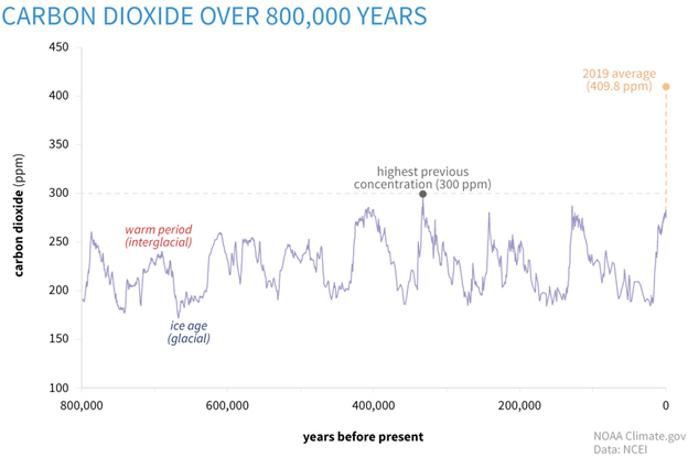
Even more remarkable is the fact that the pace of change has been accelerating. Since 1981, global temperature has increased an average of 0.18°C per decade, more than twice the average since 1880.18 We can get a more detailed picture of this acceleration by looking at one of the underlying drivers of global temperature: atmospheric CO2.By combining data from Greenland ice cap cores with an even longer ice record from the Antarctic ice cap, we can string together a continuous history of atmospheric CO2 that goes back about 800,000 years (Fig. 1.7). Prior to the agro-industrial revolution that began in the late 1700s, levels of CO2 had fluctuated within a range between about 172 and 300 ppm. These fluctuations corresponded with a fairly dynamic period in Earth’s climate that saw the repeated advance and retreat of massive glaciers in the Northern Hemisphere. This pattern changed distinctly after the agro-industrial revolution. At the start of the nineteenth century, atmospheric CO2 was about 280 ppm. By 2019, it had climbed to 409.8 ppm,19 the highest it has ever been in the annals of the ice core record, and likely the highest it has been since about the middle of the Pliocene, 3-5 mya.20Even in comparison to the dynamic swings in atmospheric CO2 seen in the ice cores, the recent spike in CO2 is exceptional. During the first decade of the twenty-first century, atmospheric CO2 increased about 100 times faster than during any other period of the ice record, including during the surge in CO2 that heralded the end of the last ice age and the beginning of the Holocene. Since about 1950, the annual rate of increase has averaged about 2 ppm per year, but this average rate masks the fact that the pace of emissions has been accelerating over that time. In the 1960s, the annual rate of increase was about 0.7 ppm per year; by the start of the twenty-first century, it had increased to 2.1 ppm per year; and in 2016, it reached a record 3.0 ppm per year, although the growth rate has been slightly less in recent years—2.5 ppm per year in 2019.21
We can estimate the level of atmospheric CO2 even further back in time using Earth System models and proxy metrics that are correlated with CO2 abundance, such as the density of stomata on fossilized leaves, although these approaches yield much less certain estimates than the ice core record. Despite the uncertainty, atmospheric CO2 has been impressively high at times in the past. In the early Eocene (51 mya), the latest estimate pegs atmospheric CO2 at 1,400 ppm.22 CO2 levels might even have been well above 3,000 ppm during the early epochs of the Paleozoic era. Compared to these, the current level of atmospheric CO2 might seem unremarkable, but the future (or past) is closer than it appears. If we continue emitting CO2 at the current pace, we will reach 950 ppm by the end of this century.23
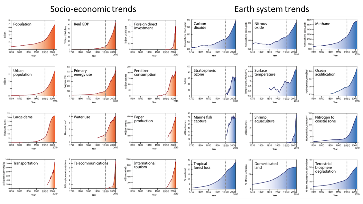
The rate of change has also been accelerating for other Earth System metrics. There was a coordinated acceleration in Earth System change that started abruptly around the middle of the twentieth century. The acceleration in Earth System change coincided with equally dramatic accelerations in traits that characterize the social, political, and economic organization of human societies, such as the global integration of trade, increased urbanization, and intensive energy use (Fig. 1.8). This broad spike in human societal and planetary change that occurred after 1950 has been termed the Great Acceleration.24 Don’t gloss over the word acceleration. The Earth is not only changing quickly; it is also on a runaway trajectory. That puts immense pressure on us as well as the rest of life to try and keep up.
In their final report, the Anthropocene Working Group argued that 1950, the start of the Great Acceleration, would be a good time point to mark the start of the Anthropocene. It is after 1950 that we begin to observe significant global changes across a wide range of Earth System metrics. Not everyone agrees with their suggestion, and there are other ideas. The Anthropocene Working Group’s recommendations are currently still just recommendations. The full International Commission on Stratigraphy must now decide whether to declare a new epoch, and if so, when it should start. As you might suspect of an organization of geologists, they are not particularly impatient to do so.
1.3 Force Multipliers
Section 1.3: Force Multipliers
A remarkable aspect of the Great Acceleration in Earth System change is that it is being caused entirely by a single species. Only a handful of other organisms over the entire history of the planet are even in the same league in terms of their impact. Cyanobacteria living 295 mya are a contender.
When they evolved oxygen-producing photosynthesis, they started to fill the world with the previously rare and highly toxic chemical O2. This eventually caused atmospheric O2 levels to spike about 250 mya (an episode known as the Great Oxygenation Event). This triggered one of the greatest mass extinctions Earth has ever seen. Although the Great Oxygenation Event was perhaps one of the most profound ways that life has ever shaped the planet, its timing was remarkably sedate compared to the changes taking place in the Anthropocene. Our understanding of the exact timing is pretty sketchy, but it seems that cyanobacteria started pumping out O2 many years before its levels spiked in the atmosphere. Many, many years before—perhaps something like half a billion years before.25 Moreover, cyanobacteria seem to have been only one part (albeit a critical one) of a complex series of interactions and feedbacks between many parts of the Earth System that played out over millions of years.
In comparison, the speed of human-driven change has been nearly instantaneous. It is even more amazing that we have been able to cause such a fundamental shock to the Earth System even though our numbers are relatively modest. As of 2019, there were about 7.7 billion people on the planet. That is a trifling rounding error compared to the estimated 3 trillion trees on the planet.26 Yet, just like those trees, we have become integral players regulating the global climate system. How have we managed to pull off this feat?
Even though the social and ecological changes that are now taking place are dizzying, the forces and conditions that aligned to ignite the Great Acceleration developed over a long period of human history. The pathways (evolutionary, ecological, social, economic, political) that converged into making humans such a powerful force were long and convoluted. But our profound influence on the planet is generally related to three things:
- Rapid human population growth.
- Rapid technological innovation.
- Increasingly intensive resource use.
You should not think about these as isolated factors. They interact and feed back onto each other in myriad complex ways. Trying to work through all the possible interactions, feedback loops, and their consequences can make your head hurt. I will try to simplify things by exploring the history of how these forces have combined to influence just one important aspect of our interaction with the planet: how we get our food.
1.4 The Rise of Agriculture
Section 1.4: The Rise of Agriculture
For most of human history, our numbers have been few. It is difficult to know just how few, but we can make estimates based on the genetic variation present in contemporary human genomes. One analysis suggests that around 150,000 years ago, there were roughly 120,000–325,000 humans living on Earth, all of them in Africa. Our effective population size (the number of breeding individuals) was even less, perhaps as few as 12,000 people.27 This period was right after anatomically modern humans first appeared in the fossil record and about 50,000 years before migrating out of Africa.28 Even as we expanded around the world, our numbers did not grow very much. Local population sizes often got perilously low. During the Pleistocene, our numbers in Europe rose and fell with the retreating and expanding glaciers. There may have been as few as 130,00 people living in all of Europe during the Last Glacial Maximum, 23,000 years ago.29
Our rarity was in part a reflection of our limited ability to get food. Paleolithic people made their living hunting and harvesting wild foods such as game, shellfish, nuts, and fruit. Compared to your average modern city dweller, Paleolithic people were masters at this. They developed deadly stone weapons and (as I mention above) may even have promoted the growth of their favorite plants and animals in order to make hunting and foraging for them easier.
Compared to other animals, however, humans are mediocre in terms of innate physical skills. We don’t see or smell all that well, we don’t run very fast, and we are pretty weak and scrawny. About the only physical trait we have going for us is that we are exceptionally good long-distance runners. One of our most effective hunting techniques may have simply been to follow prey for long periods, pestering them with our stone arrowheads until they finally succumbed to exhaustion.30 While this strategy allowed us to carve out a niche for ourselves, it took a herculean amount of time, effort, and energy. The returns on that lifestyle in terms of net calories that could be extracted from the environment were meager. But at the start of the Holocene, we developed a new technology that would forever change our and the planet’s history: agriculture.
The development and spread of agriculture around the world is often called the Neolithic Revolution. Revolution is a good way to describe the profound impact that the transition to agriculture had on the world. It reorganized our societies, it reshaped our cultures, and it radically altered how we interact with the biosphere. But this revolution wasn’t like a modern political revolution that plays out over a few weeks and involves a few charismatic players. Instead, agriculture slowly developed over thousands of years. It also developed independently in several distant parts of the world. The first evidence that humans had successfully domesticated plants and animals dates to about 12,000 years ago in West and East Asia, followed a couple thousand years later in Mesoamerica and South America. By 8,000 years ago, independent centers of agriculture had also developed in Africa, South Asia, New Guinea, and North America.31
Despite their considerable skills, early hunter-gatherers were largely dependent on the behaviors, traits, and inconstant natures of other species for their food. With agriculture, we created a radically different relationship. We made other species dependent on us. That might not have been our explicit goal at first. We probably started out just giving a helping hand to the species and individuals we found most useful. But that general favoritism gradually became more intensive and planned. We began to manage the basic reproductive biology of our favored species, dictating when, where, and with whom they could mate. We sifted through the resulting offspring, choosing individuals with traits that were most useful to us and discarding the rest. In doing so, we developed organisms whose traits were designed to benefit us as much as the organisms themselves. We developed pigs that were fat and friendly but not very good at defending themselves from predators. We developed squash that produced large, tasty fruits but that were poor competitors for soil nutrients. We developed grasses whose seeds remained firmly attached to the plant instead of dispersing to start a new generation.
To compensate for the shortcomings of our domesticated species, we built environments specifically designed to support and nurture them. At first, the main tool we used to build domesticated habitats was our old standby, fire. But instead of setting fires to promote the natural establishment of species we liked, we used it to clear the way for our domesticated species. For example, about 7,700 years ago, the first farmers of domesticated rice in the Lower Yangtze region of China made room for their cultivated plots by burning down the alder-dominated wetlands of the region.32
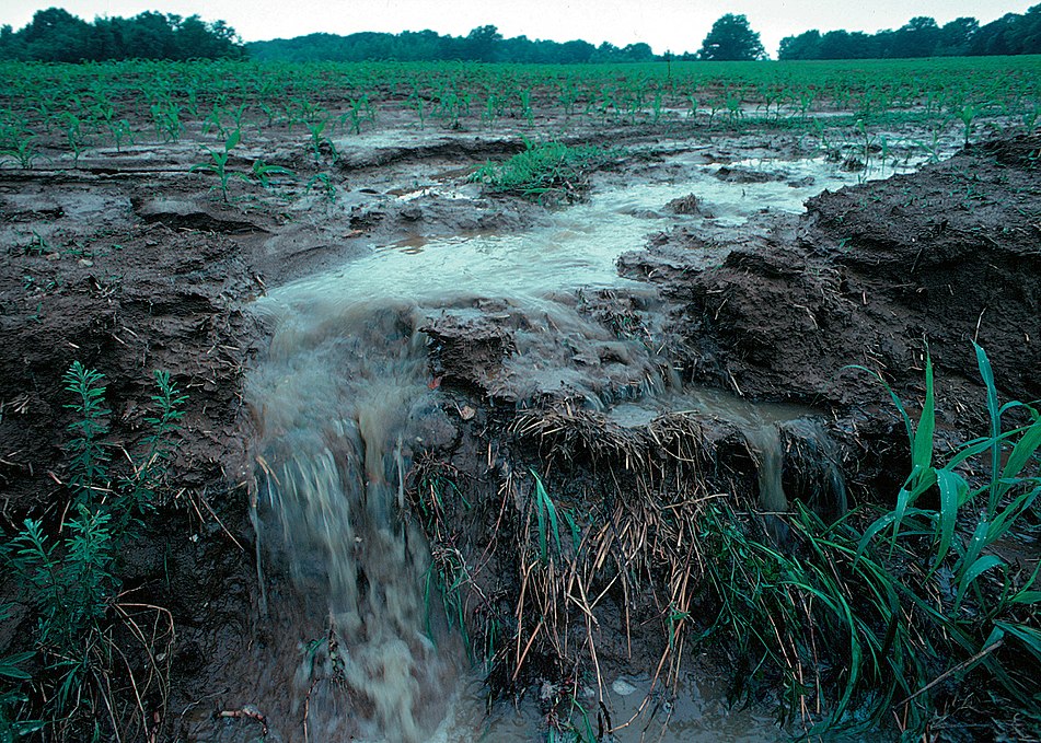
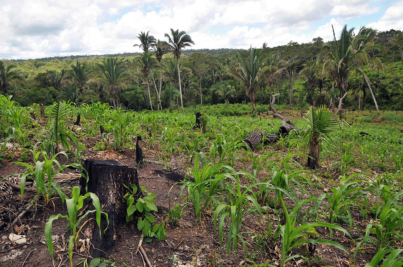
Some of the early fire-dependent farming systems probably resembled the shifting cultivation systems that are still practiced in some tropical regions today (Fig. 1.9). In these systems, cleared plots are cultivated for a few years, then abandoned and allowed to return to natural vegetation for a period. We also quickly developed more place-based systems that involved maintaining permanently cultivated fields near to where we lived. For example, the first farmers in western Norway practiced a form of shifting agriculture, but they also created more permanent cultivated fields centered around settlements.33
Maintaining permanently cultivated fields required more intensive management. We couldn’t just wait for natural processes to restore nutrient levels and reduce the herbaceous weeds that competed with our crops. There is considerable evidence that even the earliest forms of farming involved the use of fertilizers, perpetual weed management, and sophisticated water management. There is evidence that 5,900 years ago, farmers across Europe were using livestock manure and supplemental water to increase the productivity of permanently cultivated fields.34 About 7,000 years ago, rice farmers in eastern China were carefully managing the flooding and drying out of fields to maximize production.35 Around the world, early Neolithic farmers were developing sophisticated stone and wood tools that allowed them to more efficiently clear land, till soil, and harvest crops.36 All of that investment in effort and resources allowed us to transform natural landscapes into novel ecosystems that were organized primarily to feed us.
As impressive as that sounds, the benefits of farming for human well-being were at first dubious. Aficionados of the paleo diet will not be surprised to hear that hunter-gatherers had far better nutrition and overall health than the first farmers.37 Hunter-gatherers ate a diverse array of nutritious fruits, vegetables, and nuts mixed in with an occasional bit of lean meat or fish. In contrast, the first farmers ate a much more monotonous and less nutritious diet dominated by starches and grains, in part because only a handful of plant species were domesticated. In addition, the more sedentary and dense settlements that resulted from farming facilitated the spread of disease and even spurred the evolution of new human pathogens. In many cases, people probably only adopted agriculture out of desperation when the supply of game and other wild foods became scarce, either because of overexploitation or climate change at the beginning of the Holocene.
Despite the clear drawbacks, farming set in motion a cascade of events that triggered a profound shift in human demography. By co-opting the lives of other organisms, farming gave us a small escape from the daily demand and uncertainty of foraging for a meal. Instead of spending days searching for food, chasing it across long distances, or engaging it in dangerous combat, we could organize set work schedules to tend tidy plots close to home. As we got better at farming, we also got more confident that there would be enough food tomorrow, next week, or at the end of the growing season. More consistent surpluses of food freed up time for people to do other things besides tracking down ground sloths and digging for clams. Things like designing better farming techniques, inventing new tools, improving communication and record keeping, developing trade routes and knowledge networks, building cities, inventing mathematics, and pondering our existence and place in the universe. It also freed up time and resources for having babies.
In a bit of a paradox, although early farmers had a higher death rate compared to hunter-gatherers, they also had a higher birth rate. The cemeteries of early farming communities have proportionally far more juveniles in them than the cemeteries of hunter-gatherers.38 In a foreshadowing of the high-calorie diets that would plague modern human societies, folks in early farming communities ate far more calories far more consistently than hunter-gatherers. This consistent flow of calories, even if it was a bit less nutritious than a diverse paleo diet, could nevertheless feed more young mouths. In addition, a more sedentary lifestyle might have made it easier for the community to care for more children. As a consequence, the women in early farming communities gave birth to a child about every 2.5 years, compared to every 3.5 years for women in hunter-gatherer communities. The increased frequency of childbearing was a powerful demographic driver that outweighed the demographic downsides of farming, and it nudged human populations into a growth trajectory.
We can also view the agricultural advantage in a more broadly ecological way. All animals extract energy from their local environment and convert it into themselves and their offspring. The total energy available in a particular environment sets a fundamental cap on the population density of the organisms that live there. That’s why plants and animals are relatively sparse in a desert and relatively dense in a wet tropical forest. Population density is also a function of the size of individuals. Big individuals use more per capita energy than small ones. That results in an inverse relationship between body size and population density. There are always more mice around than elephants. Human hunter-gatherer populations roughly fit this size-density relationship, although their densities were on the low side compared to other land mammals their size.39 In contrast, early farming communities had population densities that were an order of magnitude higher (Fig. 1.10). Agriculture allowed us to leverage energy out of the environment in a way that no other animal could. Our design and management of agroecosystems fundamentally increased the amount of energy that flowed to us. We went from being weak competitors with other organisms to managers of our own bespoke ecosystems. It is hard to overstate the importance of that change.
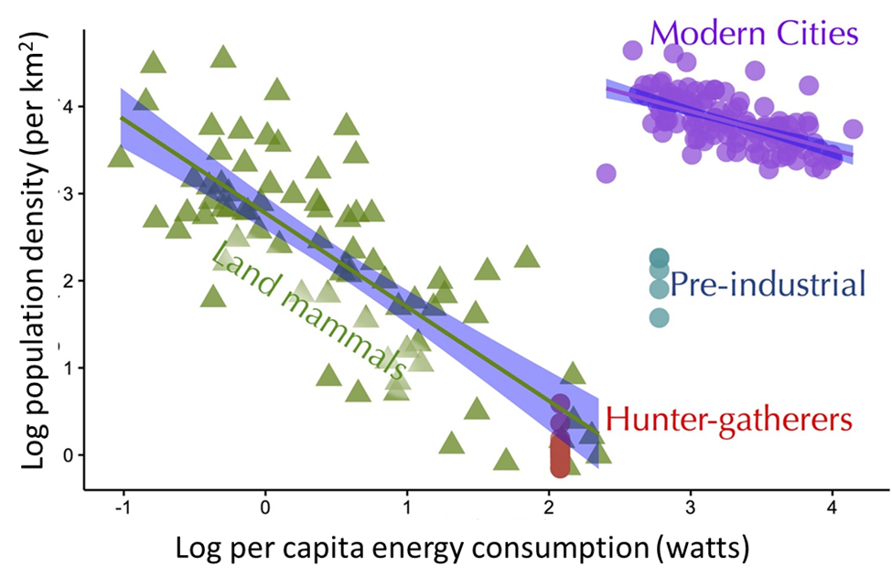
But there was yet more change to come. Modern city dwellers live at densities that are up to four orders of magnitude greater than those of hunter-gatherers, yet they consume up to two orders of magnitude more energy per capita (Fig. 1.10). How we managed that is the next stage of the story.
1.5 Agro-Industrialization
Section 1.5: Agro-Industrialization
After the transition to agriculture, human populations began to grow, but slowly. At the start of the Neolithic Revolution, there were probably about 4 million people living on Earth. Over the next 8,000 years, the population grew on average only about 0.04% per year. By the start of the Renaissance in Europe and the height of the Aztec Empire in central Mexico, the world population was less than 400 million.40 This modest population was dominated by young people in the prime of their reproductive lives—or about to enter it. In terms of fecundity alone, the human population had a lot of demographic potential. But its potential fecundity was held back by a range of limiting factors. Although agriculture greatly improved food security, it was far from perfect. Early farmers were still often powerless against the vagaries of weather and pests, so that even a modest string of cool springs or dry summers could create a crop production crisis. Conversely, good farming years often just set the stage for misery down the road. Agricultural surpluses spurred population growth, which then put intense pressure on the food system. In a story that would sadly repeat itself over most of our history, innovations in farming would generate food surpluses that fed population growth. The increased demand for food would put intense pressure on the food system to expand capacity. To meet the demand, farmers would often start growing crops on marginal land, overdraw water resources, and stop investing in soil fertility. In many cases, these unsustainable agricultural practices likely contributed to an erosion of agricultural capacity just at the moment when food demand was highest. There is a lot of suggestive evidence that agricultural management failures have contributed to many of the most tumultuous periods of social, political, and economic upheaval in history.41
But how could farmers that were skilled enough to spark population growth in the first place not be able to keep pace with demand? One significant reason was that farmers had a difficult time sustainably managing soil fertility. In shifting cultivation systems, farmers just move on to another plot when fertility declines or pests became too much of a problem. But those types of system require large amounts of land. Simultaneously maintaining fertility and agricultural output on finite amounts of arable land became a big problem that societies often failed to solve. Classic examples come from the ancient civilizations of Mesopotamia. Sumerian society rose to dominance in part because of the extensive irrigation systems it developed. That irrigation also gradually caused soils to become saline and waterlogged. The resulting decline in agricultural production contributed to a massive shift of people and political power from Sumer in the south to Babylon in the north. Babylon society fared no better. Deforestation for timber and grazing as well as large-scale tillage caused massive soil erosion that clogged the critical network of irrigation canals. Like Sumer before it, the political power and social influence of Babylon declined along with agricultural productivity.42
If the technical shortcomings of early agriculture weren’t enough to tamp down population growth, our usually filthy, cramped, and harsh living conditions; our rudimentary health care; and our propensity to violently kill each other helped do the job. But we slowly began to unfetter ourselves from these demographic constraints. A short and ecologically oriented answer for how we managed the feat is that we developed a series of technologies that allowed us to exert even more control over the natural world. We used that greater control to co-opt even more of Earth’s energy and materials into supporting our well-being. We commonly think of that process as starting in the mid-eighteenth century with the invention of mechanical tools powered by fossil fuels: the industrial revolution. The year 1750 is often used as an arbitrary date to divide the preindustrial and industrial periods of human history. Like the rise of agriculture, however, industrialization developed over thousands of years in different places and in different ways. It also was more than just steam-powered machines. Industrialization involved fundamental changes to how we organized our societies and interacted with each other. Importantly, it also changed how we grew our food. Industrialization was as much about farms as it was about factories.
We can see the early beginnings of agro-industrialization 1,700 years earlier, during the height of the Roman Empire and the Han Dynasty. Agriculture in both of those societies had already developed much of the industrialized feel and scale that it has today. Landscape-scale water systems provided flood control and irrigation water, along with clean drinking water and sanitation to city dwellers. Iron farming tools powered by domesticated animals reduced the time and human power needed to farm, allowing farm sizes to increase. Preservation techniques (such as fermentation) and transportation networks allowed food and other agricultural products to become globally traded commodities. Agricultural scientists tested new approaches to nutrient management, such as crop rotation.4344
At the height of both empires, world population was probably about 300 million people. Had agro-industrial innovation (along with the socioeconomic structures that supported it) continued to grow at the pace they were on, the Great Acceleration might have occurred much earlier. Indeed, some of the earliest evidence that humans were changing the global climate system comes from this time. Levels of methane (CH4) in the atmosphere rose significantly about 2,000 years ago, likely as a result of widespread deforestation in Europe and Asia to make way for farming and to fill a growing need for fuel in the form of firewood and charcoal.45 But for a range of reasons, both Roman and Han societies declined not long after they achieved their peaks in power and technological prowess. The resulting turmoil and displacements plunged much of the world into a long innovation hiatus that kept human population growth stagnant for more than a millennium. There is some evidence that the inability of both Roman and Han societies to sustainably manage their rapidly increasing environmental impact contributed to their demise. For example, extensive deforestation in the Huang He watershed led to massive erosion and increased runoff that eventually overwhelmed the ability of the Han government to build the effective flood control and water management systems upon which the agricultural productivity of the region was based.46
The English Industrial Archetype
It wasn’t until the seventeenth century that conditions aligned to catalyze another transformative spurt of innovation. Bursts of agricultural and technological advances began happening around the world, most notably in China and South Asia. For instance, farmers in the Yangtze Delta used fertilizer called bean cake, a byproduct of pressing soybeans for oil. The soybeans were largely grown in northern China, and then the manufactured bean cake was shipped south via a sophisticated transportation network. Partly as a result of the steady supply of external fertilizer, agricultural yields in the Yangtze Delta were nine times greater than those in England from the early 1600s through to the early 1800s.47 In South Asia, similar agricultural advances such as sophisticated irrigation systems helped support the economic rise of the Moghul Empire. In addition to food crops, Indian farmers grew a variety of raw material commodities, such as cotton and indigo, that fed a thriving globalized trade in manufactured goods, most notably textiles. In 1750, India contributed a quarter of the world’s entire industrial output.48
By comparison, the agricultural changes that were happening in England during this time were not particularly unique or advanced. Indeed, many of them were just adaptations of basic concepts that were developed thousands of years earlier in other places. But England’s story is notable for what happened next. For complicated reasons, over the next 200 years, agricultural innovation and industrialization stalled in other parts of the world while they accelerated in England. Some of the reasons for this growth reflect the negative influence of British colonialism and imperialism (see Unequal Industrialization below). But a complex array of local political, social, and economic conditions also played a role. Whatever the reasons, by the middle of the nineteenth century, England had transformed into the first fully industrialized society. The pattern that began in England would spread to become the archetype of our current world.
Although the new farming technologies that were introduced in England during the sixteenth and seventeenth centuries weren’t particularly novel, they nevertheless played a critical role in launching England’s industrial trajectory. One of the most important advances was the development of sophisticated crop rotation systems that integrated nitrogen-fixing legumes and other forage crops such as turnips, cereal grains, and livestock. During the Middle Ages in England, crop rotations were much simpler. Farmers would alternate fields between crop production and being left fallow for a year or more to restore fertility. Nitrogen-fixing species weren’t often specifically used as a way to restore fertility. Also, animals weren’t an integral part of the crop production system. They were often grazed on marginal lands and permanent communal pastures. The new, more complex rotations allowed farmers to sustainably intensify the use of agricultural land. By growing fodder cover crops such as legumes and turnips, farmers could raise livestock on the land while simultaneously restoring soil fertility and reducing weed and pest abundance. In 1700, about 20% of the arable land in England was fallow at any given time, but by the late 1800s, that figure had fallen to 4%.49 The rotation systems also allowed farmers to convert tracts of relatively low productivity single-purpose pasture into more productive integrated farmland. Other innovations included applying the scientific method to the breeding of new crop and livestock varieties, the development or refinement of mechanized farm machinery such as the automated seed drill, and the development of new fertilizer sources such as mined sodium nitrate.
The social network of English farmers was just as important as the technology itself. The intensity of information exchange and entrepreneurship made eighteenth-century England something like the Silicon Valley of its day. Although there were no formal agricultural schools, English farmers developed their own learning and technology transfer networks. They organized farm tours and exhibitions to demonstrate new approaches and share ideas. They wrote books and articles about new agricultural practices, and they developed on-farm research trials to evaluate new approaches and to adapt technologies to local conditions.50 In aggregate, all the innovation began to significantly improve the efficiency and productivity of English agriculture. In 1600, English farms had an average cereal grain yield of 8.89 bushels per acre (in wheat equivalents); by 1800, it had increased to 21.58 bushels per acre. Total cereal grain output almost tripled over that same time.51
The technical advances in farming had several important consequences. Perhaps most importantly, the increased output helped support a growing population. In 1650, the English population was about 5.3 million. That represented a rebound from the dip caused by the Black Death pandemic in the fourteenth century.51 There had been 5 million people in England at other times in the past, but never more than that. Five million people seemed to be the maximum that the English ecosystem could support, but not after 1650. By 1800, the population was 8.7 million; 50 years later, it was 16.7 million.51
The growth in agricultural output was not just used to feed people. Surpluses allowed farmers to channel more food to their farm animals, including the animals that were used to power machinery. Increasing numbers of healthy and well-fed draft animals such as horses provided power that transcended the limits of human labor alone. The growing importance of animals (horses in particular) can be seen in the statistics for oats. In medieval times, an estimated 30% of the oats grown in England were fed to animals. By 1800, the percentage had increased to 70%.52 More farm animals also allowed English farmers to produce raw materials for manufactured goods such as wool and leather. This helped farmers diversify their incomes and hedge their risks.53 Ironically, as farmers improved their efficiency, it decreased the need for farmers. The yield increases meant not only that farmers could grow more food on the same amount of land, but also that they could grow more food with roughly the same number of people. The increased mechanization and work provided by draft animals further reduced the need for human labor. This is reflected in the fact that from 1600 to 1850, the agricultural output per English farmworker steadily increased while the number of farmworkers steadily decreased.52
The changes in agricultural technology interacted with economic, cultural, and political changes to generate a wave of profound social change in England over a short period. England’s transformation during the seventeenth and eighteenth centuries was a preview of changes that would spread globally over the next two centuries. The socioeconomic patterns that emerged have become hallmarks of today’s industrialized societies. One of these is the largely privately owned and entrepreneurial nature of farms. In the Middle Ages, England (like much of the world) was organized under a feudal system. Large chunks of land were controlled by a few privileged lords and the church. These manor holdings were subdivided into small strips that were farmed by indentured tenants who rented (in a broad and euphemistic sense of the word) the land from the lord. Much of the rest of the land was managed communally, and all the members of the manor community had rights to use it and took responsibility for managing it. This basic arrangement persisted even as feudalism declined as a formal social system. All of that began to change in the seventeenth century. The change was partly catalyzed by the increased profitability of farming. There began to be more value in what the land could produce than in how much rent a lord could squeeze out of impoverished peasants. Communal lands began to be reorganized into privately held farms. These tended to be much larger than the tiny strips of land that most feudal peasants had. They also were run more like commercial businesses, with an eye toward shaving costs and maximizing returns.
Just as the privatized and more efficient farms needed fewer people to run them, emerging manufacturing industries began to need workers. Mills and factories offered an alternative livelihood for the rising number of increasingly marginalized farmworkers. During the Middle Ages, 80% of England’s population lived on farms. At the start of the eighteenth century, slightly more than half the population still lived on farms. Then, in just over 100 years, England was transformed from a rural agrarian society into an urban industrial one. In 1850, just 20% of England’s population still lived on farms.52 Today, most of the world’s population lives in cities, but globally that has only been the case since the start of the twenty-first century.
England’s new urbanites were geographically separated from sources of food. An integrated system developed to reconnect them with farmers. Extensive transportation networks linked farmers to distributers, storage facilities, and retailers. Improvements in storage, sanitation, and preservation allowed for additional time between when food was harvested and when it needed to be eaten. An organized system was developed to price commodities and make sure everyone got paid. The English market for agricultural commodities as well as manufactured goods also became increasingly connected to other markets around the world. Of course, global trade had existed for thousands of years. But the difficulties and high costs of transportation, low agricultural outputs, and restrictive laws tended to keep markets regional and insular. This was particularly so for bulky and perishable food. That began to change in the eighteenth century, and England was right in the middle of it. The global trade in wheat is an example.
In the 1700s, a fledgling trade in wheat developed between England and its American colonies. By the late 1700s, American wheat supplied up to 4% of England’s wheat consumption.54 The American Revolution put a kink in the expanding trade. Another factor was a product of global interconnection itself. The Hessian fly (Mayetiola destructor), a serious pest of wheat and other cereal grains, had been introduced to North America, supposedly in the straw bedding of Hessian troops fighting in the American Revolution. The fly caused serious crop losses in America and contributed to an English ban on American wheat imports in an effort to keep the pest out of England.54 Despite that hiccup, the global trade in wheat continued to expand, and by the mid-nineteenth century, it had become a global commodity. Consumers were no longer tied to buying local.
More than a third of the wheat consumed in England during the mid-1800s was imported.54 As a result, the price of wheat became global as well. Before the nineteenth century, wheat prices varied a lot between regions, and the price fluctuated more or less independently in response to local conditions, such as weather and politics. By the start of the twentieth century, wheat prices in different—even distant—parts of the world became more synchronized.55 As a result, the daily lives of people became more globally interdependent. A crop failure in Russia could raise the income of farmers in the United States and increase the cost of bread for residents of London.
Unequal Industrialization
Despite a remarkable spurt of industrialization during the nineteenth century, the Great Acceleration in global social and Earth System metrics was still a century away. In part, that was because the spread of industrialization around the world was patchy and uneven. England’s comprehensive transformation was an anomaly. In other regions, the suite of technological, social, and economic changes developed in unique and often slower ways. For example, although the United States was rapidly developing its manufacturing and industrial infrastructure in the nineteenth century, it was still primarily an agrarian society. The vast majority of its population was rural, and more than half of its working-age population was either employed or enslaved on farms.56 England’s unique status was not simply a result of idiosyncratic circumstances. It was also a conscious product of imperialism.
England and other European countries weaponized industrialization as a way to secure new markets and raw materials for their agricultural and manufactured goods. Their industrial advance became intricately linked and dependent on the political and economic subjugation of other people around the world.57 For example, in the mid-1800s, English workers were weaving textiles using cotton grown by enslaved people in the Americas. British military and political power simultaneously forced open markets around the world for their artificially low-priced textiles, undercutting local textile industries and cotton farmers.58
In the twentieth century, the global inequity in industrialization began to diminish as countries expelled colonial rulers. Many countries, such as India, made industrialization an explicit goal of their independent development.59 The political upheaval of the twentieth century created, at least in some respects, a more equitable world. More of its people were free to choose their own political, social, and economic paths. Given the freedom to choose, most countries (with a few exceptions) embarked on a period of industrialization that mirrored the one England had pioneered.
That included changes to their agricultural practices. Starting in the 1950s, newly industrializing countries were assisted in that by a coordinated set of research, education, and technology transfer programs that would come to be called the green revolution.60 The explicit goal of these programs was to spread the yield and output benefits of the new agro-industrial systems to less industrialized regions like Asia. The green revolution was centered around plant-breeding programs that produced improved crop varieties that were explicitly designed to work within an industrialized system. As the twentieth century developed, that agro-industrial system became increasingly dependent on two things: nitrogen and energy.
1.6 Nitrogen and Energy
Section 1.6: Nitrogen and Energy
Ongoing and rapid technological innovation was an important aspect of the agro-industrialization that swept the world. In aggregate, these innovations fundamentally reshaped our relationship to the biosphere in just as profound a way as our initial invention of agriculture had. Many of these technological advances were incremental. For instance, increasingly efficient farm equipment made with new materials such as steel continued to reduce the per capita effort needed to farm. Two innovations were radically transformative. We figured out a way to inexpensively synthesize ammonia from nitrogen gas, and we developed systems to readily generate massive amounts of energy.
Nitrogen Fertilizer
Throughout all of human history, farmers have struggled to maintain soil fertility. Nitrogen has been the biggest challenge because it is critical for plant growth, but it quickly leaves fields in various ways—not the least being in the harvested crop itself. The eighteenth century saw sophisticated and effective approaches to maintain crop nitrogen levels. These involved variations on using animal manure and nitrogen-fixing plants to restore field nitrogen. Pairings were distinctly local, with systems like animal-integrated rotation in England, rice-fish in Asia, and legume-maize in Mesoamerica. But these systems have inherent regulating feedbacks that create a powerful constraint. In order to increase crop production, we have to concomitantly increase manure or legume production to provide the necessary nitrogen. Nitrogen management in these systems is fundamentally a zero-sum game.
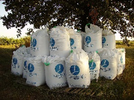
There were a couple of available nitrogen sources that did not involve these feedbacks. One was seabird manure, or guano. Seabirds forage over vast expanses of ocean but nest in a few dense colonies on land, often using the same spot over thousands of years. Seabird guano deposits provide a way to transfer a bit of the vast marine nitrogen supply to our terrestrial agroecosystems. Humans still commonly use marine nitrogen sources in agriculture, such as fish-derived fertilizers used in organic production. The other source of external nitrogen available to nineteenth-century farmers was geologic.
Organisms usually quickly suck up any loose biologically reactive nitrogen. Under a few unique environmental circumstances, however, such as hyper-arid conditions, reactive nitrogen in the form of nitrate can accumulate as geologic deposits over hundreds of thousands of years. Guano and nitrate fertilizers gave farmers access to biologically reactive nitrogen that wasn’t part of the ecological feedbacks of their local farms. They could restore field fertility without having to raise more farm animals or put a field into a nitrogen-fixing cover crop. Not surprisingly, both guano and nitrate became highly sought-after and fought-over commodities in the nineteenth century.61 Unfortunately, their supplies are both limited and costly to extract and ship. The largest deposits of both are located along the Pacific coast of South America, a long way from most of the world’s industrialized agriculture in the nineteenth century.
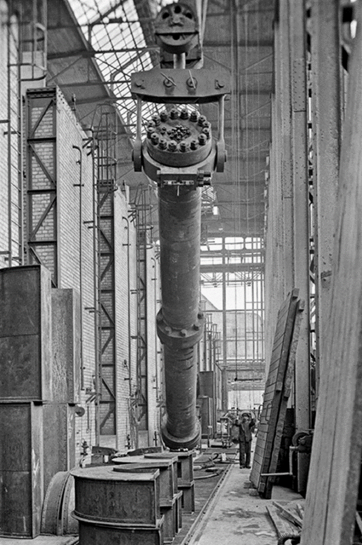
Things radically changed in the twentieth century with the development of the Haber–Bosch process, which enabled the production of inexpensive and seemingly unlimited amounts of nitrogen fertilizer. The invention was emblematic of industrialization. Fritz Haber figured out a chemical process for converting atmospheric nitrogen to ammonia using hydrogen, catalysts, and high pressure. Up until then, only a relatively few microorganisms had evolved the ability to fix nitrogen, and almost all life on the planet was directly or indirectly dependent on them. We became significantly less dependent on them after Haber’s invention. Haber’s process was developed on a small laboratory scale; Carl Bosch turned it into an industrial operation. The chemical company BASF constructed the first industrial ammonia reactor at their brand-new Oppau factory in 1913 (Fig. 1.11). In 1914, they produced 30 metric tons of ammonia per day.62 Most of their production that year went to manufacture explosives for use in World War I. A few decades later, World War II again sucked up most of the world’s ammonia production. When the war ended and the physical damage it had caused was repaired, manufacturers shifted their production to fertilizer.
The ready supply of vast amounts of biologically reactive nitrogen profoundly changed agriculture in many parts of the world. For the first time in history, farmers could consistently supply the nitrogen needs of their crops no matter how much nitrogen the crop demanded or how many acres they planted. With that in mind, crop breeders developed nitrogen-hogging crop varieties that were explicitly designed to take advantage of the all-you-can-eat nitrogen buffet that farmers could provide. Farmers also could devote fewer of their finite resources such as land to growing biological sources of nitrogen, and in many regions, they began to rely less on complex rotations and integrated animal systems to maintain soil fertility.
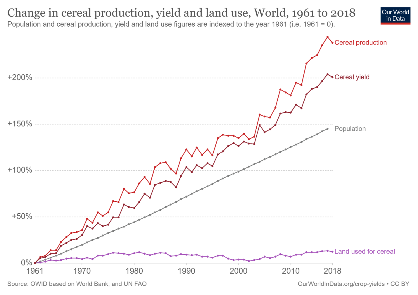
The combined result has been a dramatic increase in crop yields. For example, average global cereal grain yield has increased 175% since 1961 (Fig. 1.12). Some of those yield increases occurred in regions that were rapidly industrializing and the focus of green revolution programs. But even countries whose agro-industrialization was more developed experienced similar yield increases. For example, between 1961 and 2014, wheat yields in the United Kingdom increased by 142%.63 The yield improvements have allowed farmers to produce a lot more crops without a concomitant increase in the land needed to grow them. From 1961 to 2014, global cereal production increased 280%, while the amount of land used to grow cereal crops increased only 16%.63 Over that same period, overall crop production (grains, fruits, vegetables, fiber, etc.) rose 3.5 times, while the amount of land being farmed increased only 1.1 times.64 Not all of the increases have been the direct result of Haber–Bosch nitrogen, and it is difficult to precisely estimate its relative importance compared to other factors. Still, nitrogen fertilizer has played a significant role in increasing food availability. One study estimated that in 2008, about 48% of the human population was fed by crop production made possible by Haber–Bosch nitrogen.65
Energy
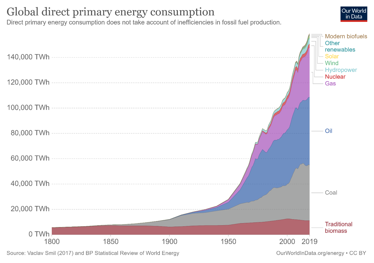
A series of technical innovations starting mainly in the nineteenth century increased our ability to find, extract, and make practical use of fossil fuels. We certainly made use of the energy windfall. Our overall energy consumption has increased dramatically since the nineteenth century (Fig. 1.13). That energy has strongly shaped almost every aspect of our global society, not the least one being agriculture. The new agro-industrial production systems, particularly those that arose after 1950, required vast amounts of energy. The list of their energy needs includes some obvious things such as running mechanized machinery and transporting harvests to market. It also includes some less obvious things, such as the energy needed to produce pesticides and fertilizer. In the early twenty-first century, just running the Haber–Bosch process accounted for about 1% of our global energy consumption and CO2 emissions.66 There are also many indirect and embedded energy costs that support agriculture, such as the energy used to build transportation, irrigation, and communication networks.
Agriculture has always required energy. But the shift to fossil fuels has been transformative. Right up through the early beginnings of agriculture, the amount of food humans could extract from the environment was limited by the energy that physical bodies could provide. It didn’t help that 20% of the energy the human body uses goes to powering big brains instead of brawny muscles.67 An important innovation was the domestication of draft animals that significantly augmented our limited physical abilities. Still, draft animals also need to eat, which constrains how much we can leverage their power to help generate excess food in the same way that using animals as a source of fertilizer does. Energy derived from fossil fuels removed that inherent biological constraint. We could tap into the accumulated residual energy fixed by ecosystems in Earth’s distant past. It was like inheriting a windfall from a rich aunt you didn’t know you had. But unlike many a trust fund youth, we collectively used our inherited energy in a range of productive ways; contributing to the prodigious growth in agricultural yields was one of the most important.
Another important aspect of the energy system that developed was that fossil fuels became more than just a source of energy. They became part of a highly interconnected agro-industrial system. This is partly because fossil fuels (i.e., various forms of hydrocarbons) are handy for doing organic chemistry. For example, not only are fossil fuels used to heat and pressurize Haber–Bosch reactor vessels, but they also provide one of the main raw ingredients. The hydrogen used in the Haber-Bosch process is derived primarily from natural gas (methane). In a process called steam reforming, methane is combined with water and a nickel catalyst to produce hydrogen gas and carbon monoxide. The ready supply of hydrocarbons from fossil fuels helped catalyze a period of amazing innovations in organic chemistry that produced an array of new chemical compounds. Just as importantly, parallel innovations in industrial engineering allowed the new chemicals to be inexpensively mass-produced. After the Haber–Bosch process, the most significant of these industrial innovations for agriculture was the development of a range of chemical insecticides and herbicides.
From a broader perspective, agriculture became a component part of a broad industrial system that extended far beyond farm fields. The increases in agricultural yields after 1950 largely reflect our ability to augment the energy and material flows of our current agroecosystems with additional flows derived from fossil fuels.68 Large segments of our agricultural system became as dependent on the constant flow of fossil hydrocarbons as they were on sunshine and water.
1.7 A Golden and Gilded Age
Section 1.7: A Golden and Gilded Age
It is always difficult to weigh the significance of recent history compared to that of the more distant past. Proximity often distorts our perceptions. We tend to bestow far more importance to events that we have directly experienced. At the same time, we often underestimate or even fail to notice changes that have accumulated over our lifetimes. Still, even accounting for our nearsighted perspective, some of the most rapid and significant changes in the history of humanity have occurred during just the past 100 years or so. You can probably trace some of the changes in your own family history. My grandfather grew up poor in a rural Greek village helping his large extended family grow olives on a tiny farm. He left Greece as a young man looking for a better life. He met his wife in Panama, and they later migrated to Detroit, Michigan. He became a barber, cutting the hair of factory workers; she became a seamstress. They bought a house, took vacations to see family back in Greece and Panama, and sent their two kids to college. Eventually, they retired to Florida, where they lived in a subdivision that a few years before had been an orange grove and a few decades before that had been a pine savannah.
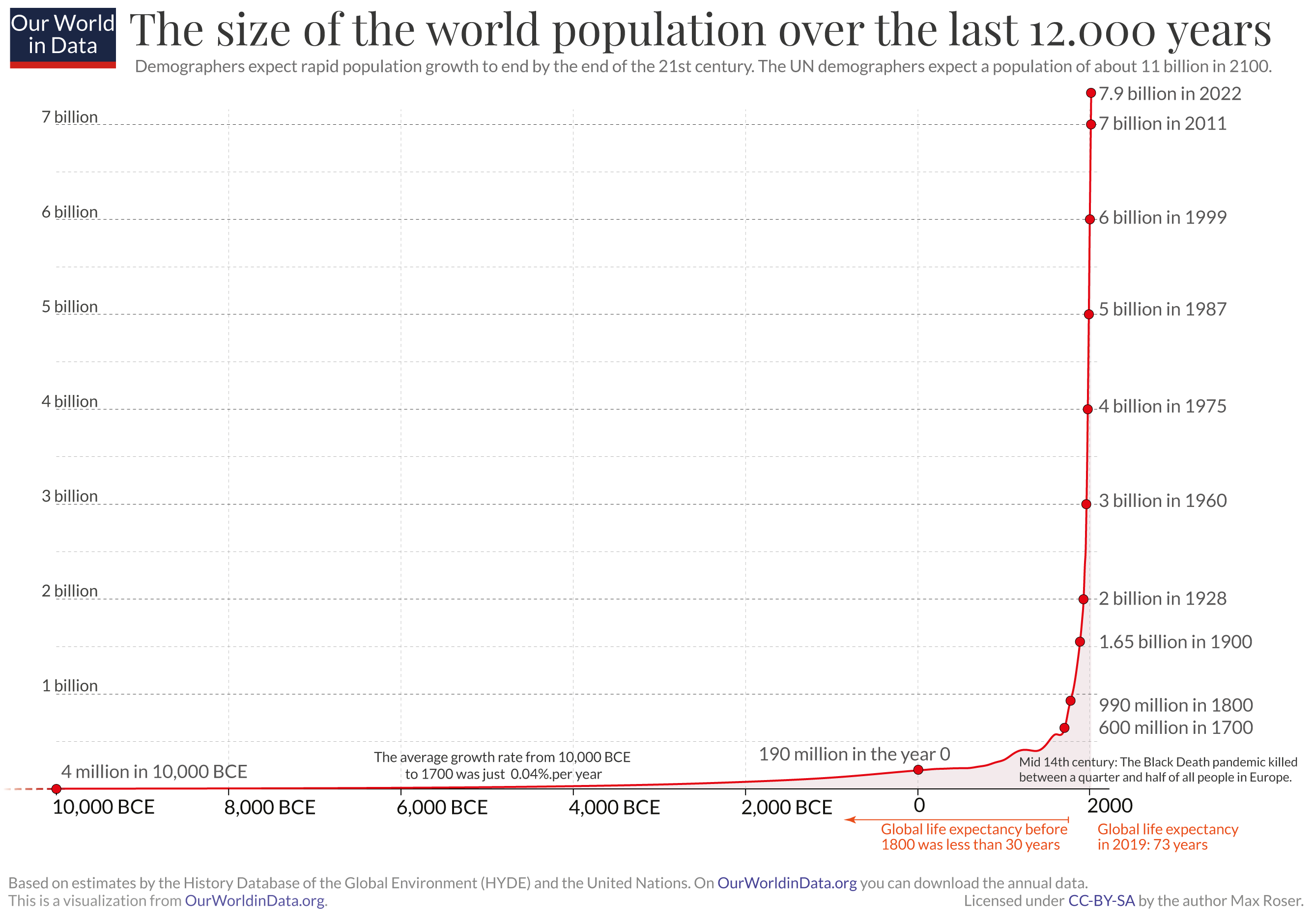
The magnitude and speed of some of these changes are described a bit more quantitatively (if dryly) in the socioeconomic statistics of the Great Acceleration (Fig. 1.8). We don’t have a lot of reliable data that extend back more than 100 years, but what we do have suggests that many of these changes are unprecedented in our history. Our current extended period of population growth is one example (Fig. 1.14). Although the population boom that we are currently experiencing became most noticeable in the twentieth century, it actually started a couple hundred years earlier, at the start of the eighteenth century, and at first it wasn’t particularly notable. We had experienced modest population booms in the past, but something always eventually nipped them in the bud. One common cause has been our inability to sustainably increase agricultural production to match rising demand for food. Medieval Europe provides a good example.
By the fourteenth century, Europe had recovered from the worst of the turmoil caused by the collapse of the Roman Empire, and this led to a population boom. Food systems in many regions were stretched to capacity. Then a series of extraordinarily wet years starting in 1314 contributed to crop failures that caused widespread food shortages and famine.69 A series of wars and the Black Death added to the woes. By the end of the fourteenth century, Europe’s population may have been half of what it was at the start of the century70 The boom in the eighteenth century was different. In a dramatic departure from our entire previous history, our population just kept growing. Moreover, the speed at which it was growing kept accelerating. By 1962, there were more than 3 billion people, and the world population was growing at an astounding 2.2% per year.
All population growth spurts are triggered by an excess of births over deaths. In the eighteenth century, the excess was created as deaths declined while births remained high. Many of the technological and social changes associated with agro-industrialization improved our living conditions in ways that reduced deaths, particularly of young children. These included radical improvements in health care, public sanitation, and housing. The net result was a global accumulation of people, mostly young ones. The growth caused alarm, in part because it was largely being driven by factors not directly tied to the food supply. Many people thought that it was just a matter of time before the perennial problem of an overstretched food system reared its head again. Most notable among these pessimistic prognosticators were Thomas Malthus in the eighteenth century71 and later Paul Ehrlich in the twentieth century.16 Both warned that human society faced impending periods of starvation, suffering, and conflict as the demand for food outstripped our ability to provide it.
A Golden Age
Thankfully, Malthus and Ehrlich underestimated the snowballing power of agro-industrialization. Throughout the period of unprecedented human population growth, our agricultural output increased at an even faster pace (Fig. 1.12). In 1968, when Ehrlich published his warning in a book titled The Population Bomb,16 the average per capita food supply was about 2,334 kcal/person/day; by 2013, food supply had risen to 2,884 kcal/person/day,73 despite the fact that there were 3.6 billion more people.
It’s understandable that Malthus and Ehrlich got their predictions so wrong. The accelerating pace of technology and innovation that kept the food supply ahead of population growth was a radical departure from the entire past human experience. Things have changed even more radically than the statistics on food supply may suggest. We didn’t just maintain living standards under a crush of new people, we substantially improved them for billions of people. This prosperity can be seen in another remarkable aspect of our recent demography. Just as population growth was booming past 2% per year in the 1960s, it then began to decline. Contrary to what Malthus and Ehrlich had predicted, the slowing population growth wasn’t caused by more deaths but by fewer births. We started having fewer babies and having them increasingly later in life. Since the 1960s, the global average birth rate has been declining, steadily narrowing the differential between births and deaths, and slowing population growth. By 2019, annual global population growth had declined to just over 1%. If the trend continues, the total human population should plateau around 11 billion people at the start of the twenty-second century.74 Population growth is one of the few Earth System metrics running counter to the Great Acceleration.
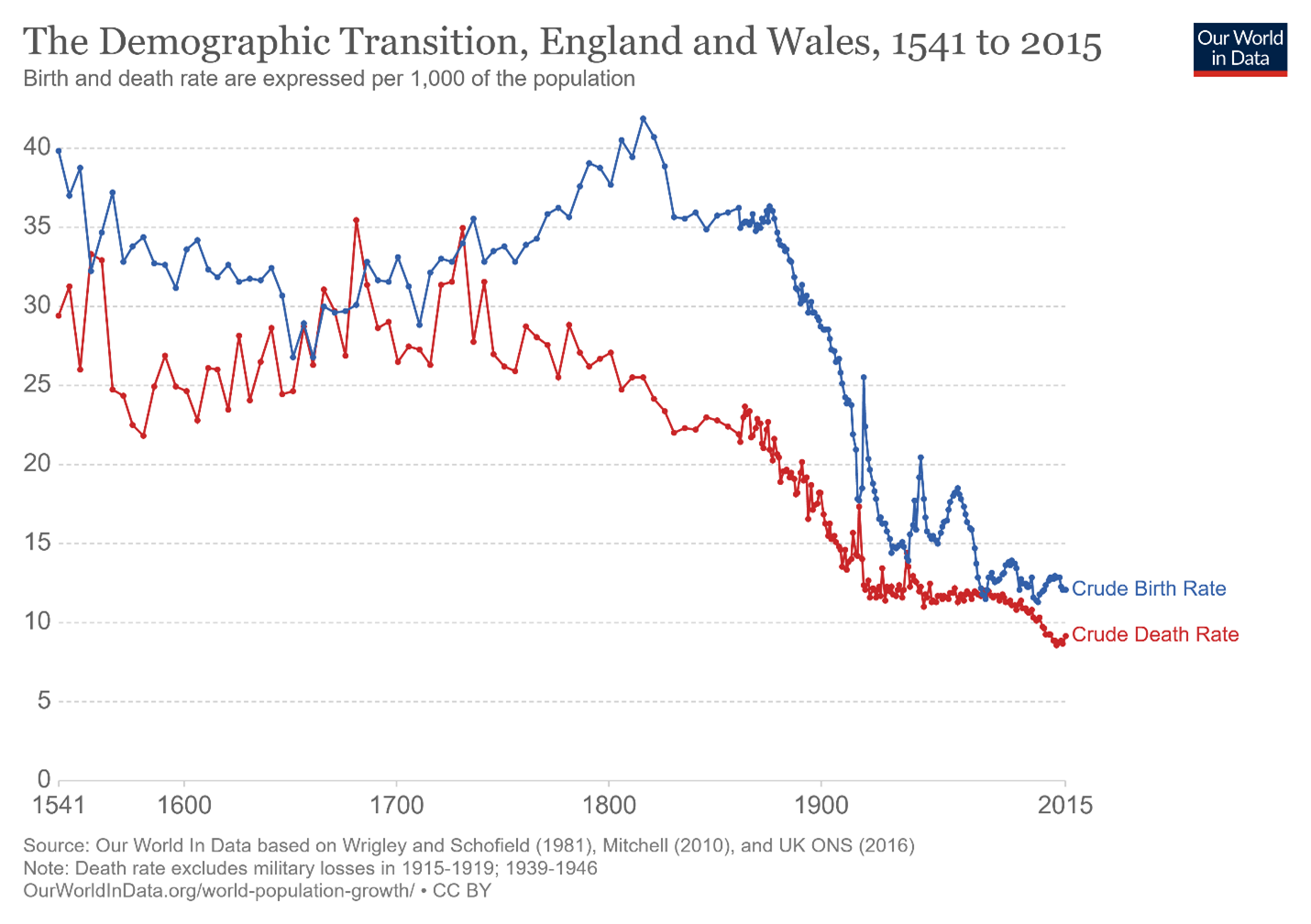
The sequence of declining death rate followed later by declining birth rate that played out globally over the past 300 years or so has been replicated in individual regions at different times. In almost every case, the demographic shift closely corresponds with the progression of agro-industrialization of the society.75 England provided the first example (Fig. 1.15). Demographers have given this distinctive pattern the rather prosaic name of the demographic transition. But its universality seems to reflect a profound change in our relationships with each other and the planet. Notably, this modern demographic transition is the mirror image of the demographic shift that happened when we invented agriculture. Back then, our adoption of agrarian lifestyles first triggered an increase in birth rates followed later by an increase in death rates.76
The causes of the modern demographic transition are a complex mix of economic, social, and cultural changes that collectively made people wealthier, healthier, and more secure. Science, technology, and political movements that prioritized public welfare all decreased the risk of dying for increasing numbers of people. The subsequent decline in birth rate is a little harder to understand.
In part, it reflects the greater autonomy that significant numbers of people have gained over their lives. Critically, that includes women. As women became more equal participants in all aspects of society, they gained greater control over their reproductive and economic decisions. Having a child became much more of an individual choice instead of a social obligation for cementing communal or economic alliances, or a burden imposed by gender inequality or crushing poverty.The broad improvement in our well-being began first in England, but it has spread globally. That can be difficult to appreciate given how many people are still desperately poor.
In 2017, 689 million people (9.2% of the world population) lived on less than $1.90 (international dollars) per day. International dollars standardize purchasing power; one international dollar anywhere in the world has the same purchasing power that one US dollar has in the United States. That is a level of extreme poverty that deprives people of basic human needs such as food, clean water, and health care. About 44% of us are a little better off than that but still struggle to meet basic needs.76
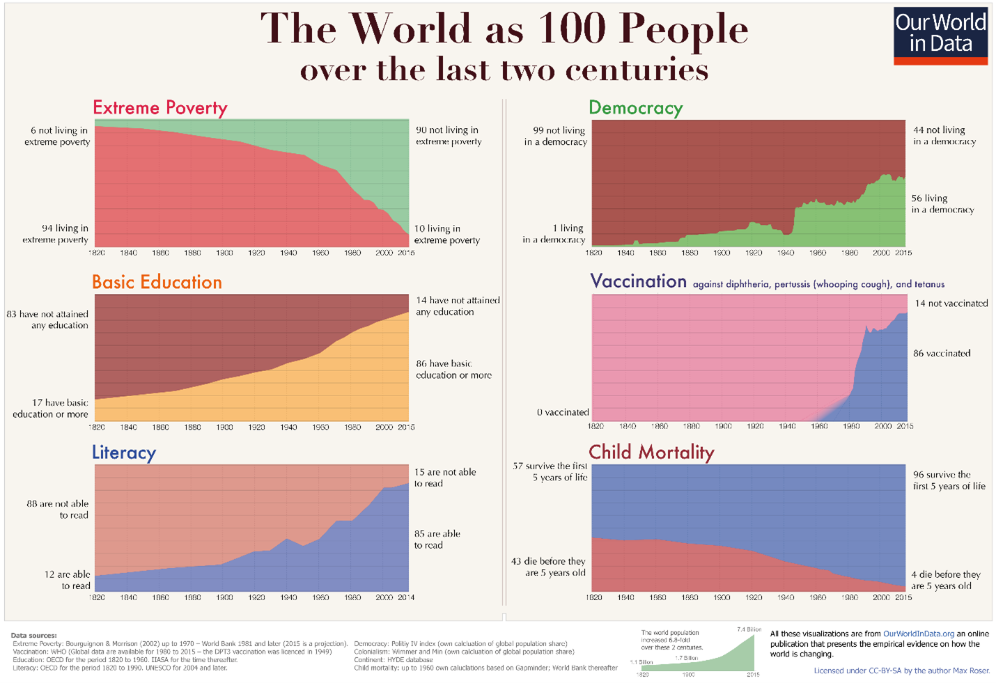
It is perhaps shocking to realize that those numbers reflect a vast improvement. Over most of our history, almost everyone lived in extreme poverty, with only a tiny elite living privileged lives. In 1820, an estimated 84% of the world’s people lived in extreme poverty. Even as late as the 1980s, more than 40% of us were extremely poor. But over the past 200 years, the proportion of people living in extreme poverty has steadily declined even as our total population boomed. Similar trends have also occurred for other aspects of well-being (Fig. 1.16). Over the same period, billions of people have moved out of poverty altogether to become middle class.
Middle class is an amorphous term, but one definition is a level of income that allows people to meet their basic needs and still have some money left over to spend on other things. Those include physical things such as houses, refrigerators, or motorcycles, as well as incorporeal things such as the occasional vacation, a subscription to an entertainment streaming service, or the financial flexibility to go back to school. More than half of the world is now middle class or rich.77 The reduction in poverty continues, but for the first time in decades, severe poverty is expected to increase as the result of the COVID-19 pandemic.78 Watch the talk by Hans Rosling in the Additional Resources for an eloquent description of the momentous increase in global prosperity that has taken place mostly since the 1950s.
Borrowed Wealth
The widespread improvement in human well-being is one of our greatest achievements. But the close association between our manipulation of the Earth System and our social achievements such as poverty reduction creates a number of philosophical and moral questions. Exploring those questions is mostly beyond the scope of this book, yet it is important not to lose sight of them. How we interpret and come to terms with these questions will shape not only human society but also the future ecology of the planet.
One significant issue that we must address is that our changes to the Earth System are beginning to compromise our own well-being. By themselves, the statistics of change in Figure 1.8 and Tables 1.1 and 1.2 don’t describe what the implications of those changes are. One broad way of contextualizing the change is to compare current conditions and trajectories with those of the past. More specifically, we can compare current conditions to those that have prevailed over the past 10,000 years, during which time we developed much of what we now view as our humanity. We have largely designed our social, economic, political, and technological systems to operate optimally under a relatively narrow range of environmental conditions that have existed for most of the Holocene. Our human systems are also supported by a specific suite of functions and services that the Earth System has been providing in characteristic ways over that period. Presumably, the further that we push environmental conditions beyond Holocene conditions, the greater stress we put on the ability of our human systems to support our well-being. In addition, as we increasingly change conditions, we risk degrading the biophysical feedbacks that help stabilize the Earth System. This could in turn drive even more changes that are largely outside of our ability to influence.
Using Holocene conditions as a reference, scientists have defined planetary boundaries for Earth System components that, if exceeded, risk tipping the Earth System into a radically different state that would significantly threaten our well-being (Table 1.3). Collectively, these planetary boundaries define a known safe operating space for humanity.79 As you might suspect, defining planetary boundaries involves a fair bit of uncertainty. We can’t set boundaries for some Earth System components because we don’t yet clearly understand how changes to the component influence the system. The large amount of plastic that we are adding to the Earth is one example. For other components, we have a basic understanding of how changes to them influence the Earth System, but we are uncertain about important details. Biodiversity loss is a good example. We are still broadly uncertain about how much and what type of biodiversity we can lose before Earth System functions are radically compromised. For other components, we have a far clearer picture of the risks. Climate is one example. Based on our detailed understanding of past atmospheric CO2 concentrations (Fig. 1.7), we have good reason to believe that the planetary boundary for atmospheric CO2 should be 350 ppm. Between 350 and 550 ppm is a zone of uncertainty, where our risks are elevated but not fully understood.79 We are currently in that zone of uncertainty (409.8 ppm in 2019), and we are indeed experiencing a range of disruptions linked to climate change, such as increased wildfire risk, more intense weather, and disruptions to our agricultural systems.23
| Estimated Range of Safety for Planetary Boundaries of Planet Earth as of 2015. | |||
|---|---|---|---|
| Earth System Component [measurement] | Safety zone | Planetary Boundary | Current Value |
| Freshwater use (blue water consumption) |
4000 km3 yr–1 | 4000–6000 km3 yr–1 | Still in the Safe Zone Measurement: ~2600 km3 yr–1 |
| Stratospheric ozone (% of preindustrial level) |
< 5% | 5%–10% | Safe, but not as safe as it could be: Measurement: <5% |
| Climate (atmospheric CO2 concentration) |
75% | 75–54% | Worrisome: Measurement: 62% |
| Biodiversity (extinctions) |
< 10 E/MSY | 10–100 E/MSY | Problematic: Measurement: 100–1000 E/MSY |
| Biogeochemical flows (human N fixation) |
62 Tg N yr–1 | 62–82 Tg N yr–1 | Straight Super Dangerous: Measurement: ~150 Tg N yr–1 |
Another way to think about planetary boundaries is that they define the limits to how much we can sustainably convert the Earth System into our well-being. As we use the Earth System to generate our well-being, we push Earth System metrics toward the planetary boundaries. Going past the boundaries risks compromising the Earth’s ability to continue providing services in the amounts and forms that we have become accustomed to. These risks are often not immediately apparent. Complex feedbacks exist both within and between the Earth System and our human system that create considerable time lags as well as other uncertainties.80 In addition, the further that we push the Earth System in new directions, the less likely it is that we will be able to easily reverse conditions. For example, many scientists worry that we are pushing the climate system toward multiple tipping points that could trigger abrupt changes to the climate regime that will largely be beyond our ability to control.81 As a result, many of the consequences of our current use of the Earth System will be borne by future generations. We are currently subsidizing our current well-being by taking a lien out against our children’s well-being. It is a debt that we have no intention of ever repaying ourselves.
A Gilded Age
The burden we are leaving future generations is not the only moral problem with the way that we use the Earth System. Another is that the benefits and costs of our use are not equally shared among us. The safe operating space below planetary boundaries is narrow. Few of us would be happy with a world where our impact on the Earth System was minimal but where most of us lived in extreme poverty. Ideally, there is a safe and just space where we use enough of the Earth System to provide all of us a fundamental level of well-being, but not so much that we push the Earth System beyond its biophysical boundaries. The economist Kate Raworth has described this sweet spot as the Anthropocene doughnut (Fig. 1.17). We are currently much more in the hole than the doughnut. Even as we are exceeding several planetary boundaries, we are falling short in several aspects of human well-being. That pattern reflects fundamental inequalities that still exist in our society.
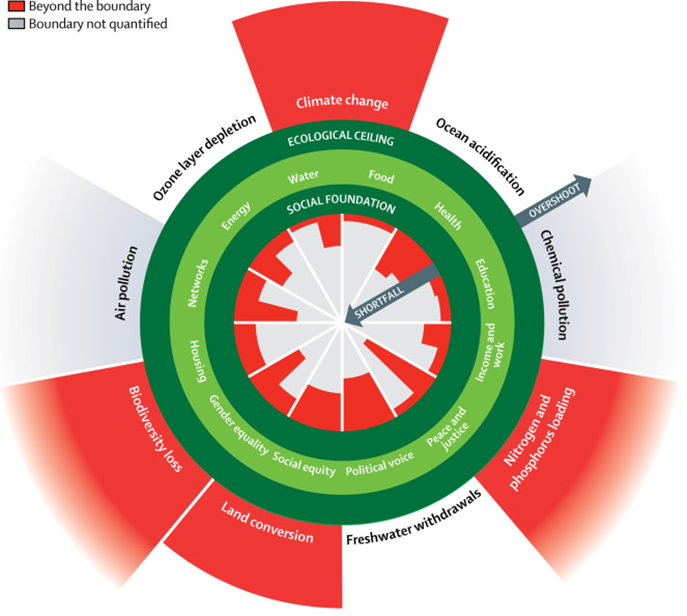
Roughly half of us struggle to get the basic things such as food and clean water that the other half of us take for granted. Even more unfairly, the people who have benefitted the most from agro-industrialization are also the most intensive users of the Earth System. In contrast, the poorest folks who have benefitted the least hardly register on the Earth’s ecological balance sheet. Figure 1.18 illustrates the inequality at the country scale. Some countries such as Germany and the Netherlands have achieved high levels of social well-being but disproportionately contribute to pushing us past Earth System boundaries. At the other end are countries like the Philippines that contribute almost nothing to environmental change but whose people suffer a low level of social well-being. Moreover, poor countries, as well as poor people no matter where they live, are the most vulnerable to the disruptions caused by changes to the Earth System.82 They have the least capacity to adapt to long-term environmental changes such as climate change. They also have no economic buffer that would allow them to recover from acute disturbances. For example, a recent analysis estimates that climate change threatens the lives and well-being of 19 million children in Bangladesh.83 The children live in poor communities that are predicted to suffer increased risks of flooding, storm damage, and severe drought.

Lots of countries are spread out along the gradient between the rich and poor extremes. But there is a conspicuous lack of countries in the top left corner of Figure 1.18; no country has yet achieved the ideal of sustainably providing a high level of well-being to its residents. At first glance, this paints a bleak picture of our future. It suggests that in order to achieve a more socially equitable world, we need to push the Earth System even further past biophysical boundaries. One model estimated that given the population in 2019 (7.7 billion), we could eliminate extreme poverty without significantly transgressing planetary boundaries, but if we wanted to make sure that everyone attained at least some level of middle-class life satisfaction, it would require us to push the Earth significantly past boundaries.84
Even so, there are a few reasons to think that this pessimistic view may be as wrong as those of Thomas Malthus and Paul Ehrlich. One is the fact that the relationship between well-being and resource consumption is asymptotic. We use the Earth System to generate prosperity and well-being. At low levels of well-being and Earth System consumption, there is a strong positive relationship between the two: more consumption leads to greater well-being. But growing resource consumption eventually produces diminishing returns in well-being. You can see this pattern in the asymptotic relationship between per capita CO2 and the Human Development Index (HDI) (Fig. 1.19). HDI is a statistic that incorporates three important dimensions of well-being: a long and heathy life, access to education, and a decent standard of living. Similarly, CO2 emissions integrate several aspects of how we consume the Earth System. HDI and CO2 emissions are strongly correlated when both are at low levels. But the correlation breaks down at the higher end of the scale. Someone living in the United States emits four times more CO2 than someone living in Sweden even though the two countries have nearly the same HDI. The extra CO2 emissions from the United States and other similarly positioned countries are a vast inefficiency that is pushing us past the climate planetary boundary without improving our well-being. There are similar patterns for a range of other metrics of human well-being and resource consumption. This suggests that we could vastly improve the efficiency of our well-being-generating systems. Our well-being generators include our food systems, our cities, and our overall economies.
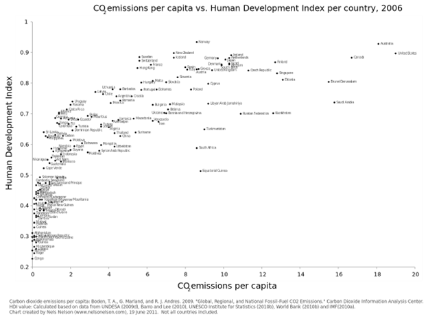
Another point for optimism is that until recently, we haven’t thought about our relationship to the planet in this way. We have tended to think about our well-being as flowing from economic and social systems that largely operated independently from the natural world. We certainly understood that we depended on the natural world for basic things such as soil fertility and clean water that we used to support our well-being. But as a global society, we often haven’t asked how our well-being in turn affected the natural world. As a result, the systems that we developed to generate our well-being were typically not explicitly designed as integrated parts of the Earth System. That was particularly the case for the agro-industrial systems that we developed over the past 200 years. Many people, including many economists, think that we can sustainably achieve a more equitably prosperous society by rethinking our basic approach. This not only involves redesigning individual well-being-generating systems, but also restructuring the overarching cultural and political structures that shape how we interact with the Earth System. For an example, see Kate Raworth’s book Doughnut Economics: Seven Ways to Think Like a 21st Century Economist (reference in the Additional Resources). Reshaping our entire global society may sound daunting, but it is no more transformative than the changes that have already happened since we left a few muddy footprints in East Africa.
Chapter Summary
The Human Age
Humans are changing Earth’s physical and biological characteristics. Many of these changes are large in magnitude, global in extent, and likely to leave a unique signature in Earth’s geologic record. As a result, many scientists now believe we are in a new geologic epoch: the Anthropocene.
- Epochs are one of the nested categories of time that geologists use to demarcate notable changes in Earth’s history (Figures 1.3, 1.4, 1.5, 1.6).
- Human activities are changing a number of Earth System properties (Table 1.1). The pace of many of these changes is remarkably quick relative to past periods of change (Table 1.2, Figures 1.6, 1.7). Since the 1950’s the pace of change has also been accelerating, an inflection point known as the Great Acceleration (Figure 1.8).
- Our ability to change the Earth System has been driven by the interaction of our rapid population growth, technological innovation, and intensive resource use.
- Our invention of agriculture and its progressive industrialization exemplify these changes. Technological innovations have allowed us to channel a transgressive amount of agroecosystem productivity to our own use (Figure 1.9, 1.10, 1.11). In the process we also transform and use prodigious amounts of resources and energy (Figure 1.13). This has helped to spur a human population boom (Figure 1.14).
- This period of rapid Earth System change has helped to improve the wellbeing of many people (Figure 1.16).
- But it has also pushed the Earth System toward critical boundaries beyond which the ability of the system to support our wellbeing is jeopardized (Table 1.3).
- The great challenge of our time is to develop ways of continuing to equitably improve the wellbeing of humanity while staying below critical planetary boundaries (Figures 1.17, 1.18).
Additional Resources
- The International Commission on Stratigraphy is where to go to catch up on the latest news about what geologic epoch we are currently living in: The International Commission on Stratigraphy.
- Will Steffen is one of the scientists who has led the effort to define the Anthropocene. He provides a nice overview in this TED talk: Will Steffen at TEDxCanberra: The Anthropocene.
- Vaclav Smil, professor emeritus at the Massachusetts Institute of Technology, has written a history of how our quest for energy shaped our society: Energy and Civilization: A History (Cambridge: Massachusetts Institute of Technology Press, 2018).
- Hans Rosling was, among other things, passionate about making our world a more equitable place. He also innovated ways of communicating science. In this TED talk, Rosling eloquently describes human population growth in the context of the demographic transition: Hans Rosling at TED: Global Population Growth, Box by Box.
- Many people are reimagining ways of making our society more just and sustainable. Economist Kate Raworth has a compelling vision she calls doughnut economics: Doughnut Economics: Seven Ways to Think Like a 21st-Century Economist (Chelsea, VT: Chelsea Green, 2017).
References
57Alam, M.S., 2012. Colonialism and Industrialization: Empirical Results. SSRN Scholarly Paper 2031131. Rochester, NY: Social Science Research Network. https://doi.org/10.2139/ssrn.2031131
47Allen, R.C., 2009. Agricultural productivity and rural incomes in England and the Yangtze Delta, c.1620–c.18201. Econ. Hist. Rev. 62, 525–50. https://doi.org/10.1111/j.1468-0289.2008.00443.x
22Anagnostou, E., John, E.H., Edgar, K.M., Foster, G.L., Ridgwell, A., Inglis, G.N., Pancost, R.D., Lunt, D.J., Pearson, P.N., 2016. Changing atmospheric CO2 concentration was the primary driver of early Cenozoic climate. Nature 533, 380–84. https://doi.org/10.1038/nature17423
2 Antón, S.C., 2003. Natural history of Homo erectus. Am. J. Phys. Anthropol. 122, 126–70. https://doi.org/10.1002/ajpa.10399
5252b52cAposolides, A., Broadberry, S., Campbell, B., Overton, M., van Leeuwen, B., 2008. English agricultural output and labour productivity, 1250-1850: some preliminary estimates. Working paper, Warwick University, Warwickshire, UK, https://ore.exeter.ac.uk/repository/handle/10871/13985.
69Baek, S.H., Smerdon, J.E., Dobrin, G.-C., Naimark, J.G., Cook, E.R., Cook, B.I., Seager, R., Cane, M.A., Scholz, S.R., 2020. A quantitative hydroclimatic context for the European Great Famine of 1315–1317. Commun. Earth Environ. 1, 1–7. https://doi.org/10.1038/s43247-020-00016-3
8Barnosky, A.D., Koch, P.L., Feranec, R.S., Wing, S.L., Shabel, A.B., 2004. Assessing the causes of Late Pleistocene extinctions on the continents. Science 306, 70–75. https://doi.org/10.1126/science.1101476
59Baru, S., 1988. State and industrialisation in a post-colonial capitalist economy: the experience of India. Econ. Polit. Wkly. 23, 143–50.
58Beckert, S., 2015. Empire of Cotton: A Global History. New York: Vintage Books.
19Blunden, J., Arndt, D.S. (Eds.), 2020. State of the climate in 2019. Bull. Am. Meteorol. Soc. 101, S1-S429.
3876Bocquet-Appel, J.-P., 2011. When the world’s population took off: the springboard of the Neolithic demographic transition. Science 333, 560–61. https://doi.org/10.1126/science.1208880
66Boerner, L.K., 2019. Industrial ammonia production emits more CO2 than any other chemical-making reaction. Chemists want to change that. Chem. Eng. News 97.
34Bogaard, A., Fraser, R., Heaton, T.H.E., Wallace, M., Vaiglova, P., Charles, M., Jones, G., Evershed, R.P., Styring, A.K., Andersen, N.H., Arbogast, R.-M., Bartosiewicz, L., Gardeisen, A., Kanstrup, M., Maier, U., Marinova, E., Ninov, L., Schäfer, M., Stephan, E., 2013. Crop manuring and intensive land management by Europe’s first farmers. Proc. Natl. Acad. Sci. 110, 12,589–594. https://doi.org/10.1073/pnas.1305918110
42Brevik, E.C., Hartemink, A.E., 2010. Early soil knowledge and the birth and development of soil science. CATENA 83, 23–33. https://doi.org/10.1016/j.catena.2010.06.011
$Broughton, J.M., Weitzel, E.M., 2018. Population reconstructions for humans and megafauna suggest mixed causes for North American Pleistocene extinctions. Nat. Commun. 9, 5441. https://doi.org/10.1038/s41467-018-07897-1
80Brown, C., Alexander, P., Arneth, A., Holman, I., Rounsevell, M., 2019. Achievement of Paris climate goals unlikely due to time lags in the land system. Nat. Clim. Change 9, 203–8. https://doi.org/10.1038/s41558-019-0400-5
*39Burger, J.R., Weinberger, V.P., Marquet, P.A., 2017. Extra-metabolic energy use and the rise in human hyper-density. Sci. Rep. 7, 43869. https://doi.org/10.1038/srep43869
61Clark, B., Foster, J.B., 2009. Ecological imperialism and the global metabolic rift: unequal exchange and the guano/nitrates trade. Int. J. Comp. Sociol. 50, 311–34. https://doi.org/10.1177/0020715209105144
*Cohen, K.M., Harper, D.A.T., Gibbard, P.L., 2020. ICS International Chronostratigraphic Chart. Episodes 36. https://stratigraphy.org/ICSchart/ChronostratChart2020-03.pdf
26Crowther, T.W., Glick, H.B., Covey, K.R., Bettigole, C., Maynard, D.S., Thomas, S.M., Smith, J.R., Hintler, G., Duguid, M.C., Amatulli, G., Tuanmu, M.-N., Jetz, W., Salas, C., Stam, C., Piotto, D., Tavani, R., Green, S., Bruce, G., Williams, S.J., Wiser, S.K., Huber, M.O., Hengeveld, G.M., Nabuurs, G.-J., Tikhonova, E., Borchardt, P., Li, C.-F., Powrie, L.W., Fischer, M., Hemp, A., Homeier, J., Cho, P., Vibrans, A.C., Umunay, P.M., Piao, S.L., Rowe, C.W., Ashton, M.S., Crane, P.R., Bradford, M.A., 2015. Mapping tree density at a global scale. Nature 525, 201–5. https://doi.org/10.1038/nature14967
28deMenocal, P.B., Stringer, C., 2016. Climate and the peopling of the world. Nature 538, 49–50. https://doi.org/10.1038/nature19471
55Dobado-González, R., García-Hiernaux, A., Guerrero, D.E., 2012. The integration of grain markets in the eighteenth century: early rise of globalization in the West. J. Econ. Hist. 72, 671–707. https://doi.org/10.1017/S0022050712000332
1616b16cEhrlich, P.R., 1968. The Population Bomb. New York: Ballantine.
65Erisman, J.W., Sutton, M.A., Galloway, J., Klimont, Z., Winiwarter, W., 2008. How a century of ammonia synthesis changed the world. Nat. Geosci. 1, 636–39. https://doi.org/10.1038/ngeo325
10Erwin, D.H., Bowring, S.A., Yugan, J., 2002. End Permian mass extinction: a review. In: Koeberl, C., MacLeod, K. (Eds.), Catastrophic Events and Mass Extinctions: Impacts and Beyond. Boulder, CO: Geological Society of America, 363–83.
60Evenson, R.E., Gollin, D., 2003. Assessing the impact of the green revolution, 1960 to 2000. Science 300, 758–62. https://doi.org/10.1126/science.1078710
11Faith, J.T., Surovell, T.A., 2009. Synchronous extinction of North America’s Pleistocene mammals. Proc. Natl. Acad. Sci. 106, 20,641–45. https://doi.org/10.1073/pnas.0908153106
64FAOSTAT, 2016. Food and Agriculture Organization of the United Nations (FAO) Food and agriculture data. https://www.fao.org/faostat/en/#data
70Fraser, E.D.G., 2011. Can economic, land use and climatic stresses lead to famine, disease, warfare and death? Using Europe’s calamitous 14th century as a parable for the modern age. In: Paavola, J., Fraser, E.D.G. (Eds.), Ecological Economics and Environmental History, special issue, Ecol. Econ. 70, 1269–79. https://doi.org/10.1016/j.ecolecon.2010.02.010
*Gaffney, O., Steffen, W., 2017. The Anthropocene equation. Anthr. Rev. 4, 53–61. https://doi.org/10.1177/2053019616688022
33Halvorsen, L.S., Hjelle, K.L., 2017. Prehistoric agriculture in western Norway—evidence for shifting and permanent cultivation based on botanical investigations from archaeological sites. J. Archaeol. Sci. Rep. 13, 682–96. https://doi.org/10.1016/j.jasrep.2017.05.011
92Higgs, K., 2017. Limits to growth: human economy and planetary boundaries. J. Popul. Sustainability 2, 15–36.
43Hsu, P.C.-Y., Xu, Z., Hsu, C., 1980. Han Agriculture: The Formation of Early Chinese Agrarian Economy, 206 B.C.–A.D. 220. Seattle: University of Washington Press.
15Jamieson, A.J., Malkocs, T., Piertney, S.B., Fujii, T., Zhang, Z., 2017. Bioaccumulation of persistent organic pollutants in the deepest ocean fauna. Nat. Ecol. Evol. 1, 0051. https://doi.org/10.1038/s41559-016-0051
*Jin, Y., Wang, Y., Henderson, C., Wardlaw, B.R., Shen, S., Cao, and C., 2006. The Global Boundary Stratotype Section and Point (GSSP) for the base of Changhsingian Stage (Upper Permian). Episodes J. Int. Geosci. 29, 175–82. https://doi.org/10.18814/epiiugs/2006/v29i3/003
77Kharas, H., Hamel, K., 2018. A global tipping point: half the world is now middle class or wealthier. Brookings Institute, September 27, 2018. https://www.brookings.edu/blog/future-development/2018/09/27/a-global-tipping-point-half-the-world-is-now-middle-class-or-wealthier/.
46Kidder, T.R., Zhuang, Y., 2015. Anthropocene archaeology of the Yellow River, China, 5000–2000 BP. The Holocene 25, 1627–39. https://doi.org/10.1177/0959683615594469
31Larson, G., Piperno, D.R., Allaby, R.G., Purugganan, M.D., Andersson, L., Arroyo-Kalin, M., Barton, L., Climer Vigueira, C., Denham, T., Dobney, K., Doust, A.N., Gepts, P., Gilbert, M.T.P., Gremillion, K.J., Lucas, L., Lukens, L., Marshall, F.B., Olsen, K.M., Pires, J.C., Richerson, P.J., Rubio de Casas, R., Sanjur, O.I., Thomas, M.G., Fuller, D.Q., 2014. Current perspectives and the future of domestication studies. Proc. Natl. Acad. Sci. USA. 111, 6139–46. https://doi.org/10.1073/pnas.1323964111
37Latham, K., 2013. Human health and the Neolithic Revolution: an overview of impacts of the agricultural transition on oral health, epidemiology, and the human body. Neb. Anthropol. 187.
56Lebergott, S., 1975. Industrialization, regional change, and the sectoral distribution of the U.S. labor force, 1850-1880: reply. Econ. Dev. Cult. Change 23, 749–50.
75Lee, R., 2003. The demographic transition: three centuries of fundamental change. J. Econ. Perspect. 17, 167–90. https://doi.org/10.1257/089533003772034943
81Lenton, T.M., Rockström, J., Gaffney, O., Rahmstorf, S., Richardson, K., Steffen, W., Schellnhuber, H.J., 2019. Climate tipping points—too risky to bet against. Nature 575, 592–95. https://doi.org/10.1038/d41586-019-03595-0
30Lieberman, D.E., Bramble, D.M., Raichlen, D.A., Shea, J.J., 2009. Brains, brawn, and the evolution of human endurance running capabilities. In: Grine, F.E., Fleagle, J.G., Leakey, R.E. (Eds.), The First Humans—Origin and Early Evolution of the Genus Homo. Vertebrate Paleobiology and Paleoanthropology. Dordrecht, Netherlands: Springer, 77–92. https://doi.org/10.1007/978-1-4020-9980-9_8
21*Lindsey, R., 2022. Climate change: atmospheric carbon dioxide. National Oceanic and Atmospheric Administration, June 23, 2022. https://www.climate.gov/news-features/understanding-climate/climate-change-atmospheric-carbon-dioxide
1818bLindsey, R., Dahlman, L., 2022. Climate change: global temperature. National Oceanic and Atmospheric Administration, June 28, 2022. https://www.climate.gov/news-features/understanding-climate/climate-change-global-temperature.
35Luo, W., Yang, Y., Zhuang, L., Gan, H., Gu, C., Huang, C., Lin, L., Zhang, J., 2020. Phytolith evidence of water management for rice growing and processing between 8,500 and 7,500 cal years bp in the middle Huai River valley, China. Veg. Hist. Archaeobotany. 30, 243-54. https://doi.org/10.1007/s00334-020-00782-2
71Malthus, T.R., 1798. An Essay on the Principle of Population, as It Affects the Future Improvement of Society. With Remarks on the Speculations of Mr. Godwin, M. Condorcet and Other Writers. London: J. Johnson.
44Margaritis, E., Jones, M.K., 2009. Greek and Roman agriculture. In: Oleson, J.P. (Ed.), The Oxford Handbook of Engineering and Technology in the Classical World. Oxford: Oxford University Press, 158-74. https://doi.org/10.1093/oxfordhb/9780199734856.013.0008
1*Masao, F.T., Ichumbaki, E.B., Cherin, M., Barili, A., Boschian, G., Iurino, D.A., Menconero, S., Moggi-Cecchi, J., Manzi, G., 2016. New footprints from Laetoli (Tanzania) provide evidence for marked body size variation in early hominins. eLife 5, e19568. https://doi.org/10.7554/eLife.19568
88McLaren, D., Fedje, D., Dyck, A., Mackie, Q., Gauvreau, A., Cohen, J., 2018. Terminal Pleistocene epoch human footprints from the Pacific coast of Canada. PloS One 13, e0193522. https://doi.org/10.1371/journal.pone.0193522
41Montgomery, D.R., 2012. Dirt: The Erosion of Civilizations. Berkeley: University of California Press.
47Morcote-Ríos, G., Aceituno, F.J., Iriarte, J., Robinson, M., Chaparro-Cárdenas, J.L., 2020. Colonisation and early peopling of the Colombian Amazon during the Late Pleistocene and the Early Holocene: new evidence from La Serranía La Lindosa. Quat. Int. 578, 5-19. https://doi.org/10.1016/j.quaint.2020.04.026
8484bO’Neill, D.W., Fanning, A.L., Lamb, W.F., Steinberger, J.K., 2018. A good life for all within planetary boundaries. Nat. Sustainability 1, 88–95. https://doi.org/10.1038/s41893-018-0021-4
49Overton, M., 1996. Agricultural Revolution in England: The Transformation of the Agrarian Economy, 1500-1850. Cambridge: Cambridge University Press.
23Pachauri, R.K., Allen, M.R., Barros, V.R., Broome, J., Cramer, W., Christ, R., Church, J.A., Clarke, L., Dahe, Q., Dasgupta, P., Dubash, N.K., Edenhofer, O., Elgizouli, I., Field, C.B., Forster, P., Friedlingstein, P., Fuglestvedt, J., Gomez-Echeverri, L., Hallegatte, S., Hegerl, G., Howden, M., Jiang, K., Jimenez Cisneroz, B., Kattsov, V., Lee, H., Mach, K.J., Marotzke, J., Mastrandrea, M.D., Meyer, L., Minx, J., Mulugetta, Y., O’Brien, K., Oppenheimer, M., Pereira, J.J., Pichs-Madruga, R., Plattner, G.-K., Pörtner, H.-O., Power, S.B., Preston, B., Ravindranath, N.H., Reisinger, A., Riahi, K., Rusticucci, M., Scholes, R., Seyboth, K., Sokona, Y., Stavins, R., Stocker, T.F., Tschakert, P., van Vuuren, D., van Ypserle, J.-P., 2014. Climate Change 2014: Synthesis Report. Contribution of Working Groups I, II and III to the Fifth Assessment Report of the Intergovernmental Panel on Climate Change. Geneva: Intergovernmental Panel on Climate Change, 151 pp.
82Pachauri, R.K., Meyer, L.A. (Eds.), 2014. Climate Change 2014: Synthesis Report. Contribution of Working Groups I, II and III to the Fifth Assessment Report of the Intergovernmental Panel on Climate Change. Geneva: Intergovernmental Panel on Climate Change.
62Pattabathula, V., Richardson, J., 2016. Introduction to ammonia production. CEP Magazine (September 2016): https://www.aiche.org/resources/publications/cep/2016/september/introduction-ammonia-production.
6Pausas, J.G., Keeley, J.E., 2009. A burning story: the role of fire in the history of life. BioScience 59, 593–601. https://doi.org/10.1525/bio.2009.59.7.10
25Planavsky, N.J., Asael, D., Hofmann, A., Reinhard, C.T., Lalonde, S.V., Knudsen, A., Wang, X., Ossa, F., Pecoits, E., Smith, A.J.B., Beukes, N.J., Bekker, A., Johnson, T.M., Konhauser, K.O., Lyons, T.W., Rouxel, O.J., 2014. Evidence for oxygenic photosynthesis half a billion years before the Great Oxidation Event. Nat. Geosci. 7, 283–86. https://doi.org/10.1038/ngeo2122
50Pretty, J.N., 1991. Farmers’ extension practice and technology adaptation: agricultural revolution in 17–19th century Britain. Agric. Human Values 8, 132–48. https://doi.org/10.1007/BF01579666
67Raichle, R., Gusnard, D., 2002. Appraising the brain’s energy budget. Proc. Natl. Acad. Sci. 99, 10,237–39.
86Raworth, K., 2017. A doughnut for the Anthropocene: humanity’s compass in the 21st century. Lancet Planet. Health 1, e48–e49. https://doi.org/10.1016/S2542-5196(17)30028-1
91Ritchie, H., Roser, M., 2018. Energy. Our World in Data, https://ourworldindata.org/energy.
6363b[63c]Ritchie, H., Roser, M., 2019. Crop yields. Our World in Data, revised June 2021. https://mjstocks.org/crop-yields.html.
3Roberts, P., Louys, J., Zech, J., Shipton, C., Kealy, S., Carro, S.S., Hawkins, S., Boulanger, C., Marzo, S., Fiedler, B., Boivin, N., Mahirta, Aplin, K., OʼConnor, S., 2020. Isotopic evidence for initial coastal colonization and subsequent diversification in the human occupation of Wallacea. Nat. Commun. 11, 2068. https://doi.org/10.1038/s41467-020-15969-4
85Roser, M., 2019. The short history of global living conditions and why it matters that we know it. Our World in Data, last updated 2020. https://ourworldindata.org/a-history-of-global-living-conditions-in-5-charts.
73Roser, M., Ritchie, H., 2013. Food supply. Our World in Data, https://ourworldindata.org/food-supply.
4040b40cRoser, M., Ritchie, H., Ortiz-Ospina, E., 2019. World population growth. Our World in Data, revised May 2019, https://ourworldindata.org/world-population-growth.
45Sapart, C.J., Monteil, G., Prokopiou, M., van de Wal, R.S.W., Kaplan, J.O., Sperlich, P., Krumhardt, K.M., van der Veen, C., Houweling, S., Krol, M.C., Blunier, T., Sowers, T., Martinerie, P., Witrant, E., Dahl-Jensen, D., Röckmann, T., 2012. Natural and anthropogenic variations in methane sources during the past two millennia. Nature 490, 85–88. https://doi.org/10.1038/nature11461
12Shakun, J.D., Clark, P.U., He, F., Marcott, S.A., Mix, A.C., Liu, Z., Otto-Bliesner, B., Schmittner, A., Bard, E., 2012. Global warming preceded by increasing carbon dioxide concentrations during the last deglaciation. Nature 484, 49–54. https://doi.org/10.1038/nature10915
27Sjödin, P., E. Sjöstrand, A., Jakobsson, M., Blum, M.G.B., 2012. Resequencing data provide no evidence for a human bottleneck in Africa during the penultimate glacial period. Mol. Biol. Evol. 29, 1851–60. https://doi.org/10.1093/molbev/mss061
24Steffen, W., Broadgate, W., Deutsch, L., Gaffney, O., Ludwig, C., 2015a. The trajectory of the Anthropocene: the Great Acceleration. Anthr. Rev. 2, 81–98. https://doi.org/10.1177/2053019614564785
79Steffen, W., Richardson, K., Rockström, J., Cornell, S.E., Fetzer, I., Bennett, E.M., Biggs, R., Carpenter, S.R., de Vries, W., de Wit, C.A., Folke, C., Gerten, D., Heinke, J., Mace, G.M., Persson, L.M., Ramanathan, V., Reyers, B., Sörlin, S., 2015b. Planetary boundaries: guiding human development on a changing planet. Science 347. https://doi.org/10.1126/science.1259855
*Steffen, W., Leinfelder, R., Zalasiewicz, J., Waters, C.N., Williams, M., Summerhayes, C., Barnosky, A.D., Cearreta, A., Crutzen, P., Edgeworth, M., Ellis, E.C., Fairchild, I.J., Galuszka, A., Grinevald, J., Haywood, A., do Sul, J.I., Jeandel, C., McNeill, J.R., Odada, E., Oreskes, N., Revkin, A., Richter, D. deB, Syvitski, J., Vidas, D., Wagreich, M., Wing, S.L., Wolfe, A.P., Schellnhuber, H.J., 2016. Stratigraphic and Earth System approaches to defining the Anthropocene. Earth’s Future 4, 324–45. https://doi.org/10.1002/2016EF000379
17Steffensen, J.P., Andersen, K.K., Bigler, M., Clausen, H.B., Dahl-Jensen, D., Fischer, H., Goto-Azuma, K., Hansson, M., Johnsen, S.J., Jouzel, J., Masson-Delmotte, V., Popp, T., Rasmussen, S.O., Röthlisberger, R., Ruth, U., Stauffer, B., Siggaard-Andersen, M.-L., Sveinbjörnsdóttir, Á.E., Svensson, A., White, J.W.C., 2008. High-resolution Greenland ice core data show abrupt climate change happens in few years. Science 321, 680–84. https://doi.org/10.1126/science.1157707
29Tallavaara, M., Luoto, M., Korhonen, N., Järvinen, H., Seppä, H., 2015. Human population dynamics in Europe over the Last Glacial Maximum. Proc. Natl. Acad. Sci. 112, 8232–37. https://doi.org/10.1073/pnas.1503784112
36Terradas, X., Piqué, R., Palomo, A., Antolín, F., López, O., Revelles, J., Buxó, R., 2017. Farming practices in the early Neolithic according to agricultural tools: evidence from La Draga Site (northeastern Iberia). In: García-Puchol, O., Salazar-García, D.C. (Eds.), Times of Neolithic Transition along the Western Mediterranean. Fundamental Issues in Archaeology. Cham, Switzerland: Springer International, 199–220. https://doi.org/10.1007/978-3-319-52939-4_8
68Tilman, D., Cassman, K.G., Matson, P.A., Naylor, R., Polasky, S., 2002. Agricultural sustainability and intensive production practices. Nature 418, 671–77. https://doi.org/10.1038/nature01014
5Trant, A.J., Nijland, W., Hoffman, K.M., Mathews, D.L., McLaren, D., Nelson, T.A., Starzomski, B.M., 2016. Intertidal resource use over millennia enhances forest productivity. Nat. Commun. 7, 12491. https://doi.org/10.1038/ncomms12491
83UNICEF Bangladesh, 2019. A Gathering Storm: Climate Change Clouds the Future of Children in Bangladesh. Florence, Italy: UNICEF.
74United Nations, 2019. World Population Prospects 2019. Accessed November 29, 2020, https://population.un.org/wpp/.
4Vaesen, K., Scherjon, F., Hemerik, L., Verpoorte, A., 2019. Inbreeding, Allee effects and stochasticity might be sufficient to account for Neanderthal extinction. PloS One 14, e0225117. https://doi.org/10.1371/journal.pone.0225117
914Waters, C.N., Zalasiewicz, J., Summerhayes, C., Barnosky, A.D., Poirier, C., Gałuszka, A., Cearreta, A., Edgeworth, M., Ellis, E.C., Ellis, M., Jeandel, C., Leinfelder, R., McNeill, J.R., Richter, D. deB, Steffen, W., Syvitski, J., Vidas, D., Wagreich, M., Williams, M., Zhisheng, A., Grinevald, J., Odada, E., Oreskes, N., Wolfe, A.P., 2016. The Anthropocene is functionally and stratigraphically distinct from the Holocene. Science 351, aad2622. https://doi.org/10.1126/science.aad2622
48Williamson, J.G., Jeffrey, G., Clingingsmith, D., 2005. Deindustrialization in the 18th and 19th Centuries. Cambridge, MA: Harvard Institute of Economic Research, Harvard University.
78World Bank, 2020. Poverty and Shared Prosperity 2020: Reversals of Fortune. Washington, DC: World Bank.
76World Bank, 2022. Understanding poverty. Last updated April 26, 2022, https://www.worldbank.org/en/topic/poverty/overview.
5151b51cWrigley, E.A., 2010. Energy and the English Industrial Revolution. Cambridge: Cambridge University Press.
53Wrigley, E.A., 2018. Reconsidering the industrial revolution: England and Wales. J. Interdiscip. Hist. 49, 9–42. https://doi.org/10.1162/jinh_a_01230
20Zhang, Y.G., Pagani, M., Liu, Z., Bohaty, S.M., DeConto, R., 2013. A 40-million-year history of atmospheric CO2. Philos. Trans. R. Soc. A 371, 20130096. https://doi.org/10.1098/rsta.2013.0096
32Zong, Y., Chen, Z., Innes, J.B., Chen, C., Wang, Z., Wang, H., 2007. Fire and flood management of coastal swamp enabled first rice paddy cultivation in east China. Nature 449, 459–62. https://doi.org/10.1038/nature06135
Media Attributions
- Figure1-1 © Fidelis T Masao et al. in Masao et al. (2007) is licensed under a CC BY (Attribution) license
- Figure1-2 © Duncan McLaren, in McLaren et al. (2018) is licensed under a CC BY (Attribution) license
- Figure1-3 © Reprinted with permission from the International Commission on Stratigraphy, cited in Cohen, et al., 2020. is licensed under a All Rights Reserved license
- Figure1-4 © Jin et al. in Jin et al. (2006) is licensed under a CC BY-NC (Attribution NonCommercial) license
- Figure1-5 © FunkMonk is licensed under a Public Domain license
- Table1-1a © Wikimedia Commons; User Synth85 is licensed under a CC BY-SA (Attribution ShareAlike) license
- Table1-1b © United States Department of Energy is licensed under a Public Domain license
- Table1-1c © Wikimedia Commons; Cjp24 is licensed under a CC BY-SA (Attribution ShareAlike) license
- Table1-1d © NASA, Goddard Institute for Space Studies is licensed under a CC BY (Attribution) license
- Table1-1e © United States Department of Agriculture, Natural Resources Conservation Service; Lynn Betts, photographer is licensed under a Public Domain license
- Table1-1f © Fredrick Rothschild is licensed under a Public Domain license
- Figure1-6 © Steffen et al. (2016) is licensed under a CC BY-NC-ND (Attribution NonCommercial NoDerivatives) license
- Figure1-7 © NOAA Climate.gov; Data from the NOAA NCEI Paleonclimatology Program is licensed under a Public Domain license
- Figure1-8 © Will Steffen, modified from Higgs (2017)
- Figure1-9 © CIAT, "Bolivia slash & burn," uploaded by mrjohncummings is licensed under a CC BY-SA (Attribution ShareAlike) license
- Figure1-10 © Reprinted from Burger, et. al (2017) is licensed under a CC BY (Attribution) license
- Figure1-11 © © BASF; BASF-Negativnummer 1795-alt is licensed under a CC BY-SA (Attribution ShareAlike) license
- Figure1-12 © Our World in Data based on World Bank, Food and Agriculture Organization of the United Nations OurWorldInData.org/crop-yields cited from Ritchie and Roser (2019) is licensed under a CC BY (Attribution) license
- Figure1-13 © Our World in Data based on Vaclav Smil (2017) and BP Statistical Review of World Energy OurWorldInData.org/energy cited from Ritchie and Roser (2019) is licensed under a CC BY (Attribution) license
- Figure1-14 © Based on estimates by the History Database of the Global Environment (HYDE) and the United Nations. On OurWorldInData.org you can download the annual data. Visualization from OurWorldInData.org OurWorldInData.org/world-population-growth; Max Roser (2019) is licensed under a CC BY (Attribution) license
- Figure1-15 © Brian Mitchell - International Historical Studeis. OurWorldInData.org/world-population-growth; Cited in Roser, et al. (2019)
- Figure1-16 © Reprinted from Roser (2019). Retrieved from OurWorldInData.org/uploads/2017/01/Two-Centuries-World-as-100-people.png is licensed under a CC BY (Attribution) license
- Figure1-17 © Downloaded from Raworth (2017) is licensed under a CC BY (Attribution) license
- Figure1-18 © Data published on https://goodlife.leeds.ac.uk/download-data and provided by O'Neill, et al. (2018). Figure CC-BY-SA Lambrinos (2022). is licensed under a CC BY (Attribution) license
- Figure1-19 © Carbon dioxide emissions per capita: Boden, T.A., G. Marland, and R. J. Andres (2009). "Global, Regional, and National Fossil-Fuel CO2 Emissions." Carbon Dioxide Information Analysis Center. HDI value: Calculated based on data from UNDESA (2009), Barro and Lee (2010), UNESCO Insitute for Statistic (2010), World Bank (2010) and IMF (2010). Chart created by Nels Nelson, 19 June 2011, CC BY-SA 3.0 is licensed under a CC BY-SA (Attribution ShareAlike) license
Masao, F.T., Ichumbaki, E.B., Cherin, M., Barili, A., Boschian, G., Iurino, D.A., Menconero, S., Moggi-Cecchi, J., Manzi, G., 2016. New footprints from Laetoli (Tanzania) provide evidence for marked body size variation in early hominins. eLife 5, e19568. https://doi.org/10.7554/eLife.19568
Those relating to bipedal apes, or to the homo genera.
Antón, S.C., 2003. Natural history of Homo erectus. Am. J. Phys. Anthropol. 122, 126–70. https://doi.org/10.1002/ajpa.10399
Roberts, P., Louys, J., Zech, J., Shipton, C., Kealy, S., Carro, S.S., Hawkins, S., Boulanger, C., Marzo, S., Fiedler, B., Boivin, N., Mahirta, Aplin, K., OʼConnor, S., 2020. Isotopic evidence for initial coastal colonization and subsequent diversification in the human occupation of Wallacea. Nat. Commun. 11, 2068. https://doi.org/10.1038/s41467-020-15969-4
Vaesen, K., Scherjon, F., Hemerik, L., Verpoorte, A., 2019. Inbreeding, Allee effects and stochasticity might be sufficient to account for Neanderthal extinction. PloS One 14, e0225117. https://doi.org/10.1371/journal.pone.0225117
Trant, A.J., Nijland, W., Hoffman, K.M., Mathews, D.L., McLaren, D., Nelson, T.A., Starzomski, B.M., 2016. Intertidal resource use over millennia enhances forest productivity. Nat. Commun. 7, 12491. https://doi.org/10.1038/ncomms12491
Pausas, J.G., Keeley, J.E., 2009. A burning story: the role of fire in the history of life. BioScience 59, 593–601. https://doi.org/10.1525/bio.2009.59.7.10
Morcote-Ríos, G., Aceituno, F.J., Iriarte, J., Robinson, M., Chaparro-Cárdenas, J.L., 2020. Colonisation and early peopling of the Colombian Amazon during the Late Pleistocene and the Early Holocene: new evidence from La Serranía La Lindosa. Quat. Int. 578, 5-19. https://doi.org/10.1016/j.quaint.2020.04.026
Barnosky, A.D., Koch, P.L., Feranec, R.S., Wing, S.L., Shabel, A.B., 2004. Assessing the causes of Late Pleistocene extinctions on the continents. Science 306, 70–75. https://doi.org/10.1126/science.1101476
Waters, C.N., Zalasiewicz, J., Summerhayes, C., Barnosky, A.D., Poirier, C., Gałuszka, A., Cearreta, A., Edgeworth, M., Ellis, E.C., Ellis, M., Jeandel, C., Leinfelder, R., McNeill, J.R., Richter, D. deB, Steffen, W., Syvitski, J., Vidas, D., Wagreich, M., Williams, M., Zhisheng, A., Grinevald, J., Odada, E., Oreskes, N., Wolfe, A.P., 2016. The Anthropocene is functionally and stratigraphically distinct from the Holocene. Science 351, aad2622. https://doi.org/10.1126/science.aad2622
Erwin, D.H., Bowring, S.A., Yugan, J., 2002. End Permian mass extinction: a review. In: Koeberl, C., MacLeod, K. (Eds.), Catastrophic Events and Mass Extinctions: Impacts and Beyond. Boulder, CO: Geological Society of America, 363–83.
Faith, J.T., Surovell, T.A., 2009. Synchronous extinction of North America’s Pleistocene mammals. Proc. Natl. Acad. Sci. 106, 20,641–45. https://doi.org/10.1073/pnas.0908153106
Shakun, J.D., Clark, P.U., He, F., Marcott, S.A., Mix, A.C., Liu, Z., Otto-Bliesner, B., Schmittner, A., Bard, E., 2012. Global warming preceded by increasing carbon dioxide concentrations during the last deglaciation. Nature 484, 49–54. https://doi.org/10.1038/nature10915
Broughton, J.M., Weitzel, E.M., 2018. Population reconstructions for humans and megafauna suggest mixed causes for North American Pleistocene extinctions. Nat. Commun. 9, 5441. https://doi.org/10.1038/s41467-018-07897-1
Jamieson, A.J., Malkocs, T., Piertney, S.B., Fujii, T., Zhang, Z., 2017. Bioaccumulation of persistent organic pollutants in the deepest ocean fauna. Nat. Ecol. Evol. 1, 0051. https://doi.org/10.1038/s41559-016-0051
Gaffney, O., Steffen, W., 2017. The Anthropocene equation. Anthr. Rev. 4, 53–61. https://doi.org/10.1177/2053019616688022
Steffensen, J.P., Andersen, K.K., Bigler, M., Clausen, H.B., Dahl-Jensen, D., Fischer, H., Goto-Azuma, K., Hansson, M., Johnsen, S.J., Jouzel, J., Masson-Delmotte, V., Popp, T., Rasmussen, S.O., Röthlisberger, R., Ruth, U., Stauffer, B., Siggaard-Andersen, M.-L., Sveinbjörnsdóttir, Á.E., Svensson, A., White, J.W.C., 2008. High-resolution Greenland ice core data show abrupt climate change happens in few years. Science 321, 680–84. https://doi.org/10.1126/science.1157707
Lindsey, R., Dahlman, L., 2022. Climate change: global temperature. Climate.gov, June 28, 2022. https://www.climate.gov/news-features/understanding-climate/climate-change-global-temperature.
Blunden, J., Arndt, D.S. (Eds.), 2020. State of the climate in 2019. Bull. Am. Meteorol. Soc. 101, S1-S429.
Zhang, Y.G., Pagani, M., Liu, Z., Bohaty, S.M., DeConto, R., 2013. A 40-million-year history of atmospheric CO2. Philos. Trans. R. Soc. A 371, 20130096. https://doi.org/10.1098/rsta.2013.0096
Lindsey, R., 2022. Climate change: atmospheric carbon dioxide. National Oceanic and Atmospheric Administration, June 23, 2022. https://www.climate.gov/news-features/understanding-climate/climate-change-atmospheric-carbon-dioxide
Anagnostou, E., John, E.H., Edgar, K.M., Foster, G.L., Ridgwell, A., Inglis, G.N., Pancost, R.D., Lunt, D.J., Pearson, P.N., 2016. Changing atmospheric CO2 concentration was the primary driver of early Cenozoic climate. Nature 533, 380–84. https://doi.org/10.1038/nature17423
Pachauri, R.K., Allen, M.R., Barros, V.R., Broome, J., Cramer, W., Christ, R., Church, J.A., Clarke, L., Dahe, Q., Dasgupta, P., Dubash, N.K., Edenhofer, O., Elgizouli, I., Field, C.B., Forster, P., Friedlingstein, P., Fuglestvedt, J., Gomez-Echeverri, L., Hallegatte, S., Hegerl, G., Howden, M., Jiang, K., Jimenez Cisneroz, B., Kattsov, V., Lee, H., Mach, K.J., Marotzke, J., Mastrandrea, M.D., Meyer, L., Minx, J., Mulugetta, Y., O’Brien, K., Oppenheimer, M., Pereira, J.J., Pichs-Madruga, R., Plattner, G.-K., Pörtner, H.-O., Power, S.B., Preston, B., Ravindranath, N.H., Reisinger, A., Riahi, K., Rusticucci, M., Scholes, R., Seyboth, K., Sokona, Y., Stavins, R., Stocker, T.F., Tschakert, P., van Vuuren, D., van Ypserle, J.-P., 2014. Climate Change 2014: Synthesis Report. Contribution of Working Groups I, II and III to the Fifth Assessment Report of the Intergovernmental Panel on Climate Change. Geneva: Intergovernmental Panel on Climate Change, 151 pp.
Steffen, W., Broadgate, W., Deutsch, L., Gaffney, O., Ludwig, C., 2015a. The trajectory of the Anthropocene: the Great Acceleration. Anthr. Rev. 2, 81–98. https://doi.org/10.1177/2053019614564785
Planavsky, N.J., Asael, D., Hofmann, A., Reinhard, C.T., Lalonde, S.V., Knudsen, A., Wang, X., Ossa, F., Pecoits, E., Smith, A.J.B., Beukes, N.J., Bekker, A., Johnson, T.M., Konhauser, K.O., Lyons, T.W., Rouxel, O.J., 2014. Evidence for oxygenic photosynthesis half a billion years before the Great Oxidation Event. Nat. Geosci. 7, 283–86. https://doi.org/10.1038/ngeo2122
Crowther, T.W., Glick, H.B., Covey, K.R., Bettigole, C., Maynard, D.S., Thomas, S.M., Smith, J.R., Hintler, G., Duguid, M.C., Amatulli, G., Tuanmu, M.-N., Jetz, W., Salas, C., Stam, C., Piotto, D., Tavani, R., Green, S., Bruce, G., Williams, S.J., Wiser, S.K., Huber, M.O., Hengeveld, G.M., Nabuurs, G.-J., Tikhonova, E., Borchardt, P., Li, C.-F., Powrie, L.W., Fischer, M., Hemp, A., Homeier, J., Cho, P., Vibrans, A.C., Umunay, P.M., Piao, S.L., Rowe, C.W., Ashton, M.S., Crane, P.R., Bradford, M.A., 2015. Mapping tree density at a global scale. Nature 525, 201–5. https://doi.org/10.1038/nature14967
Sjödin, P., E. Sjöstrand, A., Jakobsson, M., Blum, M.G.B., 2012. Resequencing data provide no evidence for a human bottleneck in Africa during the penultimate glacial period. Mol. Biol. Evol. 29, 1851–60. https://doi.org/10.1093/molbev/mss061
deMenocal, P.B., Stringer, C., 2016. Climate and the peopling of the world. Nature 538, 49–50. https://doi.org/10.1038/nature19471
Tallavaara, M., Luoto, M., Korhonen, N., Järvinen, H., Seppä, H., 2015. Human population dynamics in Europe over the Last Glacial Maximum. Proc. Natl. Acad. Sci. 112, 8232–37. https://doi.org/10.1073/pnas.1503784112
2.5mya-200kmya. Age typified by the use of chipped stone tools.
Liberalesso, T., Oliveira Cruz, C., Matos Silva, C., Manso, M., 2020. Green infrastructure and public policies: an international review of green roofs and green walls incentives. Land Use Policy 96, 104693. https://doi.org/10.1016/j.landusepol.2020.104693
The critical transition that resulted in the birth of agriculture.
Larson, G., Piperno, D.R., Allaby, R.G., Purugganan, M.D., Andersson, L., Arroyo-Kalin, M., Barton, L., Climer Vigueira, C., Denham, T., Dobney, K., Doust, A.N., Gepts, P., Gilbert, M.T.P., Gremillion, K.J., Lucas, L., Lukens, L., Marshall, F.B., Olsen, K.M., Pires, J.C., Richerson, P.J., Rubio de Casas, R., Sanjur, O.I., Thomas, M.G., Fuller, D.Q., 2014. Current perspectives and the future of domestication studies. Proc. Natl. Acad. Sci. USA. 111, 6139–46. https://doi.org/10.1073/pnas.1323964111
Zong, Y., Chen, Z., Innes, J.B., Chen, C., Wang, Z., Wang, H., 2007. Fire and flood management of coastal swamp enabled first rice paddy cultivation in east China. Nature 449, 459–62. https://doi.org/10.1038/nature06135
A form of agriculture, used especially in tropical Africa, in which an area of ground is cleared of vegetation and cultivated for a few years and then abandoned for a new area until its fertility has been naturally restored.
Halvorsen, L.S., Hjelle, K.L., 2017. Prehistoric agriculture in western Norway—evidence for shifting and permanent cultivation based on botanical investigations from archaeological sites. J. Archaeol. Sci. Rep. 13, 682–96. https://doi.org/10.1016/j.jasrep.2017.05.011
Bogaard, A., Fraser, R., Heaton, T.H.E., Wallace, M., Vaiglova, P., Charles, M., Jones, G., Evershed, R.P., Styring, A.K., Andersen, N.H., Arbogast, R.-M., Bartosiewicz, L., Gardeisen, A., Kanstrup, M., Maier, U., Marinova, E., Ninov, L., Schäfer, M., Stephan, E., 2013. Crop manuring and intensive land management by Europe’s first farmers. Proc. Natl. Acad. Sci. 110, 12,589–594. https://doi.org/10.1073/pnas.1305918110
Luo, W., Yang, Y., Zhuang, L., Gan, H., Gu, C., Huang, C., Lin, L., Zhang, J., 2020. Phytolith evidence of water management for rice growing and processing between 8,500 and 7,500 cal years bp in the middle Huai River valley, China. Veg. Hist. Archaeobotany. 30, 243-54. https://doi.org/10.1007/s00334-020-00782-2
Terradas, X., Piqué, R., Palomo, A., Antolín, F., López, O., Revelles, J., Buxó, R., 2017. Farming practices in the early Neolithic according to agricultural tools: evidence from La Draga Site (northeastern Iberia). In: García-Puchol, O., Salazar-García, D.C. (Eds.), Times of Neolithic Transition along the Western Mediterranean. Fundamental Issues in Archaeology. Cham, Switzerland: Springer International, 199–220. https://doi.org/10.1007/978-3-319-52939-4_8
Latham, K., 2013. Human health and the Neolithic Revolution: an overview of impacts of the agricultural transition on oral health, epidemiology, and the human body. Neb. Anthropol. 187.
Bocquet-Appel, J.-P., 2011. When the world’s population took off: the springboard of the Neolithic demographic transition. Science 333, 560–61. https://doi.org/10.1126/science.1208880
Burger, J.R., Weinberger, V.P., Marquet, P.A., 2017. Extra-metabolic energy use and the rise in human hyper-density. Sci. Rep. 7, 43869. https://doi.org/10.1038/srep43869
Roser, M., Ritchie, H., Ortiz-Ospina, E., 2019. World population growth. Our World in Data, revised May 2019, https://ourworldindata.org/world-population-growth.
Montgomery, D.R., 2012. Dirt: The Erosion of Civilizations. Berkeley: University of California Press.
Brevik, E.C., Hartemink, A.E., 2010. Early soil knowledge and the birth and development of soil science. CATENA 83, 23–33. https://doi.org/10.1016/j.catena.2010.06.011
The process of human civilization changing from an agrarian and handicraft economy to one dominated by industry and machine manufacturing
Hsu, P.C.-Y., Xu, Z., Hsu, C., 1980. Han Agriculture: The Formation of Early Chinese Agrarian Economy, 206 B.C.–A.D. 220. Seattle: University of Washington Press.
Margaritis, E., Jones, M.K., 2009. Greek and Roman agriculture. In: Oleson, J.P. (Ed.), The Oxford Handbook of Engineering and Technology in the Classical World. Oxford: Oxford University Press, 158-74. https://doi.org/10.1093/oxfordhb/9780199734856.013.0008
Sapart, C.J., Monteil, G., Prokopiou, M., van de Wal, R.S.W., Kaplan, J.O., Sperlich, P., Krumhardt, K.M., van der Veen, C., Houweling, S., Krol, M.C., Blunier, T., Sowers, T., Martinerie, P., Witrant, E., Dahl-Jensen, D., Röckmann, T., 2012. Natural and anthropogenic variations in methane sources during the past two millennia. Nature 490, 85–88. https://doi.org/10.1038/nature11461
Kidder, T.R., Zhuang, Y., 2015. Anthropocene archaeology of the Yellow River, China, 5000–2000 BP. The Holocene 25, 1627–39. https://doi.org/10.1177/0959683615594469
Allen, R.C., 2009. Agricultural productivity and rural incomes in England and the Yangtze Delta, c.1620–c.18201. Econ. Hist. Rev. 62, 525–50. https://doi.org/10.1111/j.1468-0289.2008.00443.x
Williamson, J.G., Jeffrey, G., Clingingsmith, D., 2005. Deindustrialization in the 18th and 19th Centuries. Cambridge, MA: Harvard Institute of Economic Research, Harvard University.
Overton, M., 1996. Agricultural Revolution in England: The Transformation of the Agrarian Economy, 1500-1850. Cambridge: Cambridge University Press.
Pretty, J.N., 1991. Farmers’ extension practice and technology adaptation: agricultural revolution in 17–19th century Britain. Agric. Human Values 8, 132–48. https://doi.org/10.1007/BF01579666
Wrigley, E.A., 2010. Energy and the English Industrial Revolution. Cambridge: Cambridge University Press.
Aposolides, A., Broadberry, S., Campbell, B., Overton, M., van Leeuwen, B., 2008. English agricultural output and labour productivity, 1250-1850: some preliminary estimates. Working paper, Warwick University, Warwickshire, UK, https://ore.exeter.ac.uk/repository/handle/10871/13985.
Wrigley, E.A., 2018. Reconsidering the industrial revolution: England and Wales. J. Interdiscip. Hist. 49, 9–42. https://doi.org/10.1162/jinh_a_01230
Sharp, P.R., 2008. The Long American Grain Invasion of Britain: Market Integration and the Wheat Trade between North America and Britain from the Eighteenth Century. Department of Economics Discussion Paper 08-20. Copenhagen: University of Copenhagen. https://doi.org/10.2139/ssrn.1277989
Bateman, P.W., Fleming, P.A., 2012. Big city life: carnivores in urban environments. J. Zool. 287, 1–23. https://doi.org/10.1111/j.1469-7998.2011.00887.x
Lebergott, S., 1975. Industrialization, regional change, and the sectoral distribution of the U.S. labor force, 1850-1880: reply. Econ. Dev. Cult. Change 23, 749–50.
Alam, M.S., 2012. Colonialism and Industrialization: Empirical Results. SSRN Scholarly Paper 2031131. Rochester, NY: Social Science Research Network. https://doi.org/10.2139/ssrn.2031131
Beckert, S., 2015. Empire of Cotton: A Global History. New York: Vintage Books.
Baru, S., 1988. State and industrialisation in a post-colonial capitalist economy: the experience of India. Econ. Polit. Wkly. 23, 143–50.
The Green Revolution, also known as the Third Agricultural Revolution, was a period of technology transfer initiatives that saw greatly increased crop yields and agricultural production. These changes in agriculture began in developed countries in the early 20th Century and spread globally till the late 1980s. Considered controversial, as several of the policies would later be remembered as colonializing and would result in monocultural practice taking hold.
Evenson, R.E., Gollin, D., 2003. Assessing the impact of the green revolution, 1960 to 2000. Science 300, 758–62. https://doi.org/10.1126/science.1078710
Clark, B., Foster, J.B., 2009. Ecological imperialism and the global metabolic rift: unequal exchange and the guano/nitrates trade. Int. J. Comp. Sociol. 50, 311–34. https://doi.org/10.1177/0020715209105144
The process converts atmospheric nitrogen (N2) to ammonia (NH3) by a reaction with hydrogen (H2) using a metal catalyst under high temperatures and pressures. This reaction is slightly exothermic (i.e. it releases energy), meaning that the reaction is favored at lower temperatures and higher pressures.
Pattabathula, V., Richardson, J., 2016. Introduction to ammonia production. CEP Magazine (September 2016): https://www.aiche.org/resources/publications/cep/2016/september/introduction-ammonia-production.
Ritchie, H., Roser, M., 2019. Crop yields. Our World in Data, revised June 2021. https://mjstocks.org/crop-yields.html.
FAOSTAT, 2016. Food and Agriculture Organization of the United Nations (FAO) Food and agriculture data. https://www.fao.org/faostat/en/#data
Erisman, J.W., Sutton, M.A., Galloway, J., Klimont, Z., Winiwarter, W., 2008. How a century of ammonia synthesis changed the world. Nat. Geosci. 1, 636–39. https://doi.org/10.1038/ngeo325
Made from decomposing plants and animals. These fuels are found in Earth's crust and contain carbon and hydrogen, which can be burned for energy. Coal, oil, and natural gas are examples of fossil fuels.
Boerner, L.K., 2019. Industrial ammonia production emits more CO2 than any other chemical-making reaction. Chemists want to change that. Chem. Eng. News 97.
Raichle, R., Gusnard, D., 2002. Appraising the brain’s energy budget. Proc. Natl. Acad. Sci. 99, 10,237–39.
Tilman, D., Cassman, K.G., Matson, P.A., Naylor, R., Polasky, S., 2002. Agricultural sustainability and intensive production practices. Nature 418, 671–77. https://doi.org/10.1038/nature01014
Baek, S.H., Smerdon, J.E., Dobrin, G.-C., Naimark, J.G., Cook, E.R., Cook, B.I., Seager, R., Cane, M.A., Scholz, S.R., 2020. A quantitative hydroclimatic context for the European Great Famine of 1315–1317. Commun. Earth Environ. 1, 1–7. https://doi.org/10.1038/s43247-020-00016-3
Fraser, E.D.G., 2011. Can economic, land use and climatic stresses lead to famine, disease, warfare and death? Using Europe’s calamitous 14th century as a parable for the modern age. In: Paavola, J., Fraser, E.D.G. (Eds.), Ecological Economics and Environmental History, special issue, Ecol. Econ. 70, 1269–79. https://doi.org/10.1016/j.ecolecon.2010.02.010
Malthus, T.R., 1798. An Essay on the Principle of Population, as It Affects the Future Improvement of Society. With Remarks on the Speculations of Mr. Godwin, M. Condorcet and Other Writers. London: J. Johnson.
Ehrlich, P.R., 1968. The Population Bomb. New York: Ballantine.
Roser, M., Ritchie, H., 2013. Food supply. Our World in Data, https://ourworldindata.org/food-supply.
United Nations, 2019. World Population Prospects 2019. Accessed November 29, 2020, https://population.un.org/wpp/.
Lee, R., 2003. The demographic transition: three centuries of fundamental change. J. Econ. Perspect. 17, 167–90. https://doi.org/10.1257/089533003772034943
A long-term trend of declining birth and death rates, resulting in substantive change in the age distribution of a population.
World Bank, 2022. Understanding poverty. Last updated April 26, 2022, https://www.worldbank.org/en/topic/poverty/overview.
Kharas, H., Hamel, K., 2018. A global tipping point: half the world is now middle class or wealthier. Brookings Institute, September 27, 2018. https://www.brookings.edu/blog/future-development/2018/09/27/a-global-tipping-point-half-the-world-is-now-middle-class-or-wealthier/.
World Bank, 2020. Poverty and Shared Prosperity 2020: Reversals of Fortune. Washington, DC: World Bank.
A boundary for human changes to land systems needs to reflect not just the absolute quantity of land, but also its function, quality and spatial distribution.
There are overall nine, but four are discussed in this chapter.
Steffen, W., Leinfelder, R., Zalasiewicz, J., Waters, C.N., Williams, M., Summerhayes, C., Barnosky, A.D., Cearreta, A., Crutzen, P., Edgeworth, M., Ellis, E.C., Fairchild, I.J., Galuszka, A., Grinevald, J., Haywood, A., do Sul, J.I., Jeandel, C., McNeill, J.R., Odada, E., Oreskes, N., Revkin, A., Richter, D. deB, Syvitski, J., Vidas, D., Wagreich, M., Wing, S.L., Wolfe, A.P., Schellnhuber, H.J., 2016. Stratigraphic and Earth System approaches to defining the Anthropocene. Earth’s Future 4, 324–45. https://doi.org/10.1002/2016EF000379
Brown, C., Alexander, P., Arneth, A., Holman, I., Rounsevell, M., 2019. Achievement of Paris climate goals unlikely due to time lags in the land system. Nat. Clim. Change 9, 203–8. https://doi.org/10.1038/s41558-019-0400-5
Lenton, T.M., Rockström, J., Gaffney, O., Rahmstorf, S., Richardson, K., Steffen, W., Schellnhuber, H.J., 2019. Climate tipping points—too risky to bet against. Nature 575, 592–95. https://doi.org/10.1038/d41586-019-03595-0
Pachauri, R.K., Meyer, L.A. (Eds.), 2014. Climate Change 2014: Synthesis Report. Contribution of Working Groups I, II and III to the Fifth Assessment Report of the Intergovernmental Panel on Climate Change. Geneva: Intergovernmental Panel on Climate Change.
UNICEF Bangladesh, 2019. A Gathering Storm: Climate Change Clouds the Future of Children in Bangladesh. Florence, Italy: UNICEF.
O’Neill, D.W., Fanning, A.L., Lamb, W.F., Steinberger, J.K., 2018. A good life for all within planetary boundaries. Nat. Sustainability 1, 88–95. https://doi.org/10.1038/s41893-018-0021-4
A summary measure of average achievement in key dimensions of human development: a long and healthy life, being knowledgeable and having a decent standard of living. The HDI is the geometric mean of normalized indices for each of the three dimensions.

.jpg)
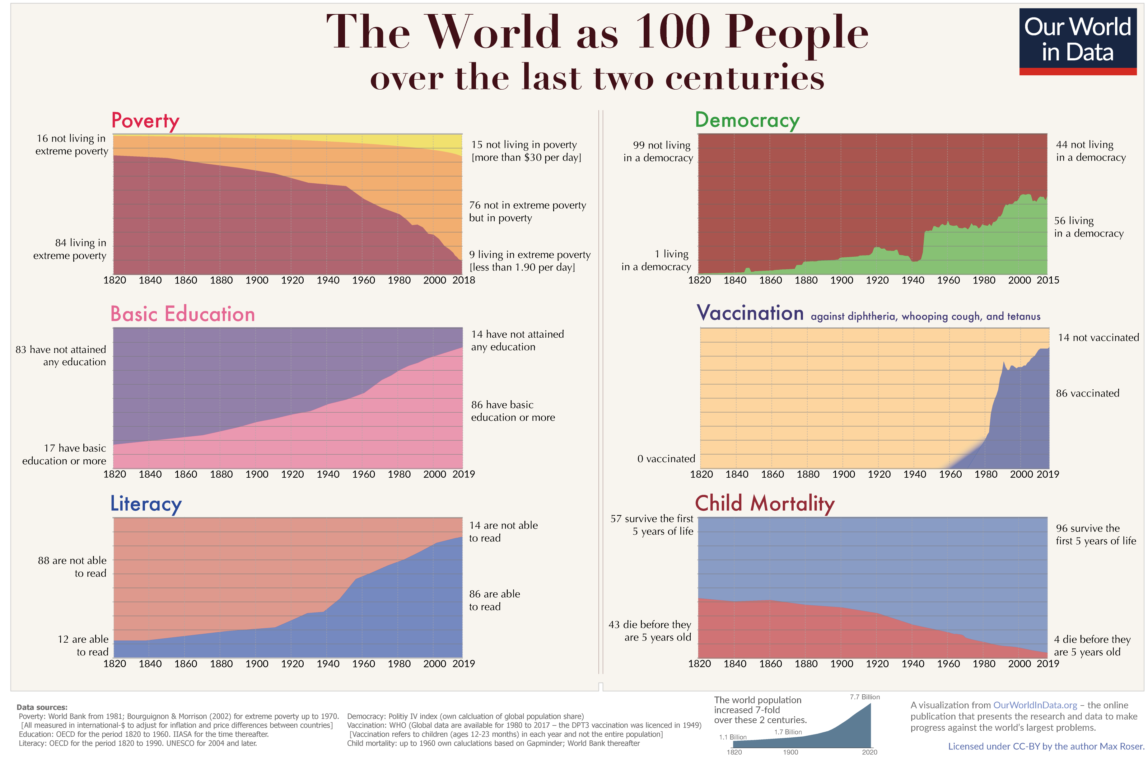