Human-Altered Systems
8 Metropolis
What Are the Characteristics of Urban Ecosystems? How Can We Build More Ecological and Equitable Cities?
Let’s meet in the city where
The rivers cross, bridges there
Let’s go float down into the stream
Of rich and poor pioneers . . .
—Sleater-Kinney, Light Rail Coyote
Sometime in the early years of the twenty-first century, someone moved to a city, triggering a major shift for humanity. For the first time ever, more people lived in a city than in the country. We don’t know who that person was or exactly when, where, or why they arrived. It could have been a baby born in Shanghai, China, a young man who left his village for a tech job in Lagos, Nigeria, or a Honduran woman fleeing poverty and violence for the relative well-being of suburban Los Angeles. Whoever they were, their arrival marked the start of a new period in human society and in our interaction with the planet. At first, all of us lived without a fixed address, extracting a living from the natural world as nomadic hunter-gatherers. Then most of us settled down as farmers and lived in small villages or scattered isolated homes. We grew food for ourselves or our close village community. Most of us never ventured beyond our village. But then, partly because we were becoming such good farmers and producing large surpluses of food, a few villages grew into towns and eventually became the first cities.
Any appeal of those first cities was likely tempered by a long list of reasons why you wouldn’t want to go to one. Even today, you are more likely to get beaten up or have your stuff stolen in a city. You are more likely to be lonely, depressed, or catch a nasty communicable disease there. You are less likely to feel connected to the natural world.1 Despite that, the lure of cities is powerful. They are centers of economic activity that attract people in need of jobs or capital. In a city, you are more likely to see something or someone new that spurs you to think of a revolutionary idea, write an epic poem, or invent a useful tool. You are more likely to find the help to market and share your ideas with other people. You are more likely to find distinct subcultures and communities of people that provide you support and acceptance or that expand your understanding of the human experience. Perhaps most basically, there is a rich variety of different things you can do in cities. Things like testing scientific hypotheses, developing ways of treating those nasty diseases, compiling compendiums of human knowledge, and dreaming about a better future world.
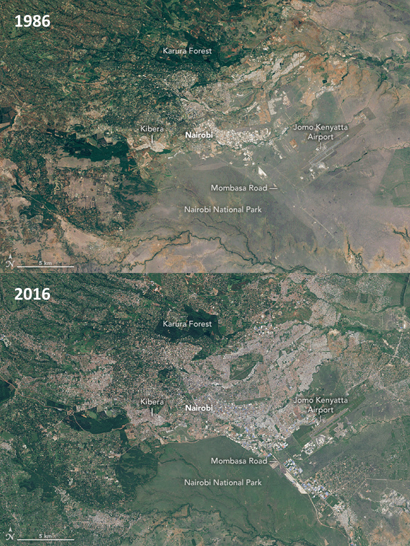
Our migration to cities was a comparative trickle at first, but it become a steady stream starting in the nineteenth century as a consequence of the agro-industrial revolution. For a range of social, political, and economic reasons, this great urban migration has occurred at different rates in different places. In England and Wales, 64% of the population was already urban by 1901; that figure rose to 82% by 1950.2 In contrast, less than 10% of Afghanistan’s population was urban in 1950.3 Like lots of other metrics, the overall global pace of urban migration sped up dramatically during the Great Acceleration after 1950. Much of this growth has taken place in Asia, Africa (Fig. 8.1), and South America, regions that remained largely rural during the early stages of agro-industrialization. For instance, just 12% of China’s population was urban in 1950. By 2018, 59% of it was. The growth of cities is continuing. By 2050, 70% to 80% of the world’s population is expected to live in cities.4b
Our move to cities is important for Earth in at least two ways. For one, urban areas are high-leverage nodes where much of our interaction with the planet now takes place. Most of the resources and biological capacity that we appropriate for our use flow through cities. Although they occupy just 2% of the land surface, cities consume 60% to 80% of the energy and 75% of the natural resources that we use. They also produce 75% of our greenhouse gas emissions.5 Second, cities are centers of innovation and novel thinking where we often try out new ideas for the first time. Ideas like strategies to help us live more sustainably on this finite planet.
In this chapter, I describe the unique characteristics of urban ecosystems. I also explore some of the ways we are reshaping our cities in more ecologically conscious ways.
8.1. What Is Urban?
Section 8.1: What Is Urban?
I live in Corvallis, Oregon, a small college town with a population (according to the 2020 census) of 59,922. It is a completely different place than the small village of Scio a few miles away (population 1,068); Phoenix, Arizona (population 1,608,139); or Los Angeles, California (population 3,898,747). But quantitatively describing why Corvallis is a sleepy college town, Scio a rural village, Phoenix a big city, and Los Angeles a global megalopolis can get a bit slippery. There are no uniformly agreed upon metrics. Perhaps the most common and straightforward metric is total population. Many government demographic offices define urban as any political delineation that meets a minimum population threshold, usually around 2,000-5,000 people. The US Census Bureau uses a threshold of 2,500. Urban can also be defined using density; one threshold is 1,500 people/km2. But these demographic metrics don’t do a good job of describing the general social vibe and geography that we associate with cities. For instance, if we apply a 2,500-person threshold to my list, only Scio is a rural place, and Corvallis gets lumped in with Phoenix and Los Angeles. If we use a density threshold of 1,500 people/km2 instead, Corvallis, with a density of 1,600/km2, just counts as urban, while Phoenix isn’t a city at all (1,198/km2), which would probably come as a surprise to its residents stuck in rush-hour traffic. I might also argue that Corvallis can’t call itself urban until it gets a decent Italian restaurant or a one-hour dry cleaner. There are a range of other metrics that more directly describe the social and economic differences between urban and rural places, such as the availability of public transportation, the percentage of residents who work in agriculture-related professions, or the density of good Italian restaurants.
All of those metrics describe urban systems in human terms, and they aren’t necessarily good descriptions of how cities function in ecosystem terms. There are, however, several broad traits of urbanization that more directly relate to ecological processes. These traits influence the physical urban environment, the types of organisms that live there, and the ecological impact that urbanization has on the Earth System. In this section, I broadly describe these traits. Then, in Sections 8.2 and 8.3, I explore more explicitly how these shape the way urban ecosystems function.
Hardscape
Perhaps the most obvious—and ecologically influential—characteristic of urban places is that they have lots of concrete (Fig. 8.2). Well, concrete and other hard materials such as asphalt, brick, steel, glass, and plastic. These hardscapes are the dominant structural elements of urban habitat. Next time you are in the downtown core of a city, estimate how much of the ground is covered by a hard surface. Most likely it will be nearly 100%. In 2020, the weight all of this human-made material was a bit more than all the biomass on Earth—about 1.1 trillion metric tonnes.6 Creating hardscape is one of the primary ways we act as strong ecosystem engineers (see Chap. 3). The hardscapes we construct interact with the flow of energy and materials in different ways than vegetated landscapes. For instance, most hardscapes are impervious to water and evaporate less water to the atmosphere than vegetated landscapes. Consequently, every time it rains, city streets are in danger of turning into raging torrents unless we construct elaborate stormwater management systems. Hardscapes also reflect, absorb, and release solar energy in unique ways; they alter wind patterns, sound patterns, and the flow of materials like dust, soot, and nutrients.
Hardscapes are closely associated with machines that generate artificial light, artificial sound, and novel chemical pollutants. Figure 3.16 maps the urban environment for the United States in terms of four of its unique physical properties: the flow of rainwater as well as local ambient temperature, sound, and nighttime light. Note how closely those maps of physical conditions align with the map of hardscape in Figure 8.2. I describe the characteristics of this physical urban environment in more detail in Section 8.2. This urban physical environment in turn influences the organisms that live there (including us), as well as the broader flow of energy and materials through the Earth System.
Sprawl
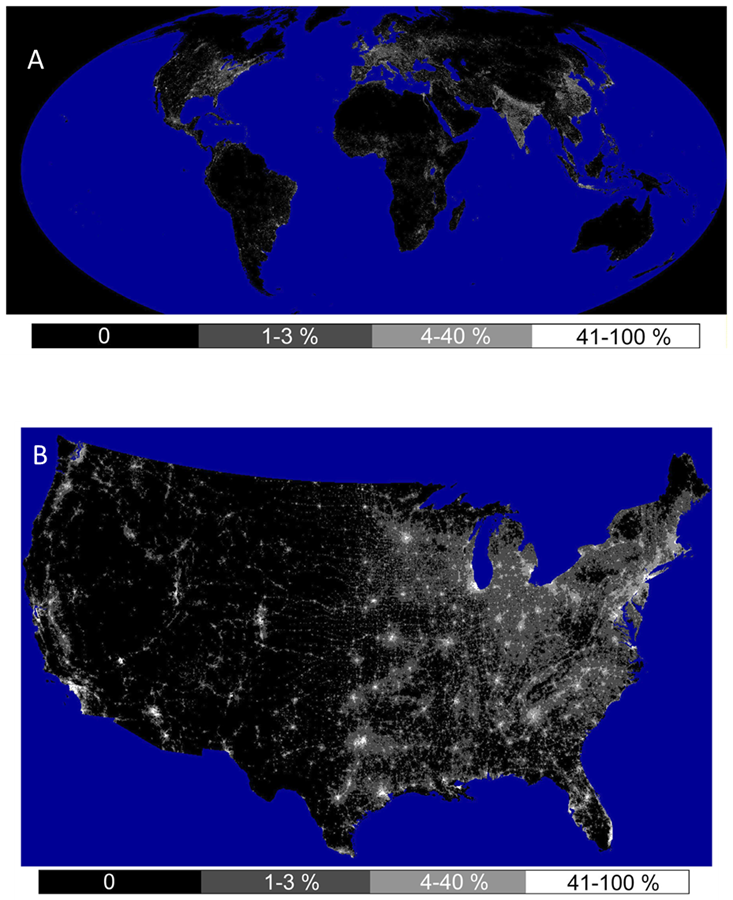
Our urban environment has a complex spatial geography. Urbanized habitat can be found in the downtown core of big cities, but also in comparatively green suburbs and even small rural towns whose main streets can proportionally have just as much hardscape and artificial light as a major commercial hub. All these bits of urban habitat are linked by a diffuse network of roads, rail lines, aqueducts, pipelines, and power lines, which themselves are urban habitats. The result is a frenetic mosaic that resembles a Jackson Pollock painting. You can see this sprawling nature in the pattern of hardscape (Fig. 8.2) as well is in the distribution of artificial light (Fig. 8.3).

Although it weighs a lot, the total area footprint of urbanization is not very big. Cities and other dense human settlements make up only 2% of the global land surface.7 The global area footprint of just the constructed hardscape is even less, about 0.5%. But the sprawling geography of urban habitat helps to give it an influence that is out of proportion to its tiny absolute footprint. It is like how the gossamer threads of a spiderweb can cause such intense annoyance if you get your face entangled in one.
One magnifying force of sprawl is habitat fragmentation. The metastasizing tendrils of urban habitat divide once-contiguous swaths of nonurban habitat into smaller chunks separated by urban environments. The spread of other domesticated landscapes such as agriculture also causes habitat fragmentation, but the sprawling nature of urban environments does a uniquely good job at it. Urban environments are also often more formidable dispersal barriers than other domesticated landscapes for many groups of organisms.
Roads are a great example of the unique ability of even small bits of urban habitat to have a significant influence. Roads are not designed for free-roaming animals, and they kill a lot of animals. We don’t have a good comprehensive global estimate, but regional totals for certain taxa suggest the scale of the carnage. In Brazil, vehicles are estimated to kill more than 8 million birds and more than 2 million mammals trying to cross roads each year.8 In Europe, the estimates are about 194 million birds and 29 million mammals.9 It’s not only vertebrates; potentially hundreds of billions of insect pollinators are killed as they cross North American roads each year.10
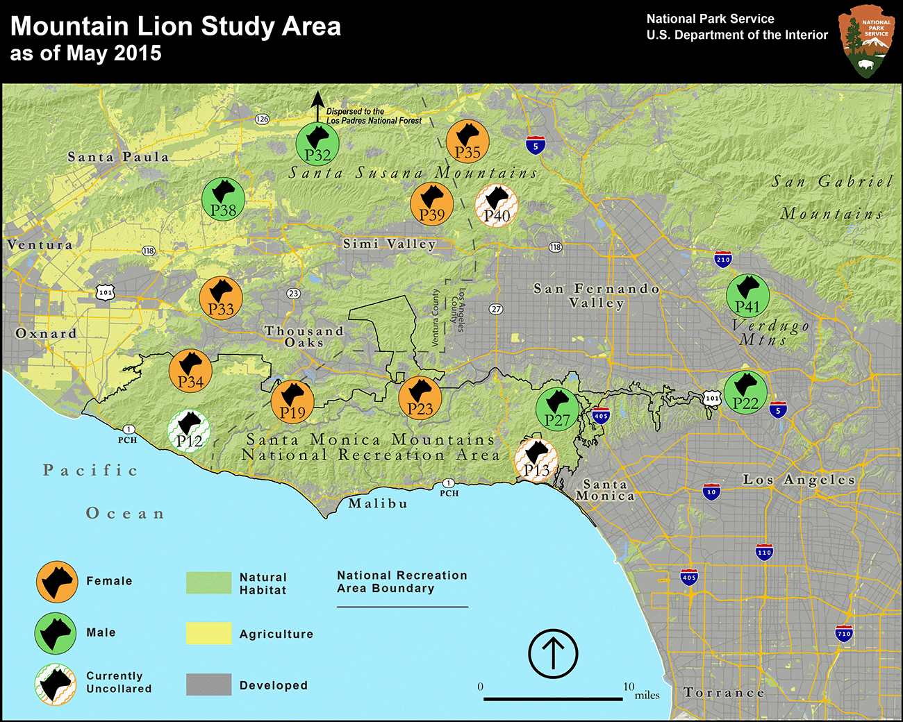
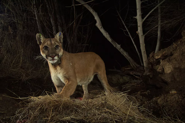
The disorienting lights, stressful noise, and strange microclimates associated with roads are intense deterrents to many organisms (see Section 8.2). Although these deterrents prevent some fatalities, they also act to separate and isolate populations. In regions with dense road networks, the resulting habitat fragments can be too small to support large numbers of individuals, particularly for species such as large predators that require extensive swaths of habitat to support their lifestyles. The reduced population sizes and the lack of gene flow (via dispersal) among populations can lead to genetic isolation and inbreeding, which can reduce the fitness of populations, leading to further population declines. Large predators are particularly susceptible to urban fragmentation. An example comes from the mountain lions (Puma concolor couguar) living in Southern California. Conditions are far from ideal for them. Their habitat is fragmented into isolated bits separated by deadly roads and largely inhospitable cities and farms (Fig. 8.4). The barriers prevent individuals from moving between the isolated habitat fragments, and the subpopulations are increasingly genetically isolated and inbred. Some individuals still attempt it move—usually young males looking to establish their own territory—but they face considerable risk when they do. They regularly end up as roadkill, eat rat poison, or get killed because they do something we don’t like, such as attacking livestock or people. The combined effects of inbreeding and the more direct sources of mortality are grinding the populations toward local extinction. Models suggest there is a roughly 21% chance there won’t be any mountain lions left in Southern California by the middle of the century.11
The tendrils of urban environment that sprawl across the landscape also create a jarringly abrupt ecotone called the wildland-urban interface (Fig. 8.5). These intersections are points of intense interaction that regulate the flow of energy, materials, and information between urban environments and other parts of the landscape. Some of these involve direct interactions between humans, our domesticated urban animals, and wildlife—many of which are unhealthy relationships for at least one of the parties. Examples include black bears (Ursus americanus) foraging through the curbside trash of Lake Tahoe, California; coyotes (Canis latrans) snacking on family pets in the suburbs of Portland, Oregon; and feral domesticated cats killing wildlife in Kakadu National Park, Australia. But the wildland-urban interface can also facilitate enriching relationships. It is one of the main places where we enjoy and benefit from the natural world. We can even form meaningful bonds with wildlife. For instance, the daily tribulations of mountain lions negotiating the complex urbanized landscape of Southern California have become a natural history reality show for its human residents.12 Many individuals have become celebrities, known by their radio-tag identifiers (Fig. 8.6). Seeing individual lions as members of the community has helped to generate broad support for efforts aimed at conserving their populations.
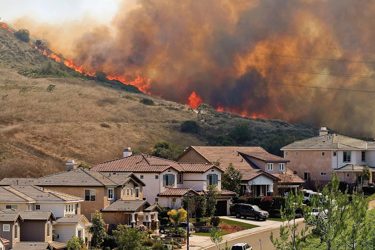
The wildland-urban interface also modifies ecosystem processes and physical conditions, which can have an influence far beyond the immediate interface itself. A salient example is wildfire. In many places, the wildland-urban interface is now where most wildland fires start, from sources such as downed power lines, discarded cigarettes, or escaped backyard fires. In California, urban metrics such as housing density explain more than half of the variation in wildfire frequency, overriding other variables such as vegetation type and climactic conditions.13 The frequency of wildfires in California has also been steadily increasing over the past century, partly as a consequence of the spread of the wildland-urban interface. We have created an entirely new fire regime, largely as a side effect of the tangled spread of urban environments. Across the entire United States, our activities now cause 84% of all wildfires, and these human-sparked fires have tripled the length of the average fire season.14
This essentially urban-driven fire regime is reshaping ecosystems across areas that extend well beyond the footprint of urban hardscape. In coastal Southern California, the spread of the wildland-urban interface has catalyzed a vicious feedback that is causing a widespread conversion of the local fire-adapted shrublands into grasslands. In addition to increasing sources of fire ignition, residential development facilitated the spread of non-native grasses. The non-native grasses dry out during the long, dry Southern California summer and provide easily flammable kindling. The combination has dramatically increased fire frequency; that is, it has decreased the time between fires at any given spot. The native chaparral shrubs of the region are exquisitely adapted to a relatively long fire interval, which historically ranged from several decades in inland mountain regions to more than a century along the coast. In many places, particularly in densely populated coastal areas, fire return intervals have been reduced to 20 years or less. This is killing the native shrubs and fostering the spread of more non-native grasses that in turn contribute to even more frequent fires.15 In addition to the ecosystem changes, the human toll of these fires is immense, in part because more of us now live so close to the conflagrations when they start. In the United States, from 1990 to 2010, the amount of land making up the urban-wildland interface grew by 33% and the number of houses in the interface grew by 41%, making it the fastest-growing land use type in the country.16
Resource Junction
Another broad characteristic of urban ecosystems is that they function as interaction nodes for energy and resources flowing through the Earth System. This exchange is another reason why urban ecosystems have a bigger influence than their area footprint might suggest. Much of the flow of energy and resources is associated with the global food system. Almost none of the food that is consumed in urban ecosystems is generated locally. Instead, cities suck in vast amounts of primary production from surrounding ecosystems. The flow involves all the materials incorporated into the biomass, such as carbon, nitrogen, and phosphorous. For example, rural residents of Ghana export roughly 3 kg of nitrogen per capita per year, while residents of Ghanaian cities import a roughly similar amount of nitrogen in the food they eat.17 There is also a virtual resource flow that involves the resources used in the production of crops but that are not necessarily incorporated into crop biomass. Water is the prime example. Most of the water we use to grow crops doesn’t get incorporated into biomass but is instead moved to the atmosphere via evapotranspiration. That consumed water is a necessary consequence of producing food. When urban residents eat, they are, in a sense, also consuming the water it took to grow the food. This virtual water is an implicit part of food commodities that are traded around the world, mostly to and through cities.18
The flow of resources is mostly one way. For instance, in 2012, Montreal, Canada, imported 3.5 gigagrams (Gg) of phosphorous embedded in food. As a result, 85% of this phosphorous eventually left the city as human feces and food waste, 2.63 Gg ended up in landfills (e.g., as sewage sludge), and 0.36 Gg was discharged to aquatic ecosystems. Only 0.09 Gg was captured and recycled—mostly for use in urban gardens and landscapes, not the more distant agroecosystems the phosphorous came from.19 Although some of the inflowing resources stay in cities for a while—like the 2.63 Gg of phosphorous that gets deposited in Montreal’s municipal landfill each year—a lot of the resources flow through into other ecosystems primarily via wastes. Important materials that flow through cities include the greenhouse gasses and other pollutants emitted by vehicles, the nitrogen and phosphorous in human feces, and the mishmash of materials such as plastics we generate as trash. Montreal does a pretty good job of keeping its phosphorous waste out of sensitive aquatic ecosystems, even if it just ends up at the dump. That is not always the case. Rapidly growing urban areas may struggle to provide appropriate infrastructure such as sewage treatment systems. For instance, only about 20% of the nitrogen and phosphorous that flows into Kumasi, Ghana, in the form of food and other biomass gets diverted out of the waste stream and sequestered in landfills. Most of the remainder flows into waterways or is emitted to the atmosphere.20
A Note on Scale and Boundaries
As with other ecosystems, the spatial scale and boundaries that define the urban environment are subjective and ad hoc. Which scale and definition is appropriate depends on the specific questions and goals. For example, if we are interested in the degree to which urban centers input resources from surrounding areas, we might choose a coarse spatial scale and distinguish urban areas from rural ones based on a political or economic metric such as municipal boundaries. If we are interested in understanding how artificial lights influence the feeding behavior of bats, however, we might choose a finer spatial scale of observation and include in our definition of “urban” the light poles in an otherwise rural village. In addition, many of the physical traits and processes that characterize urban environments are inherently spatially fuzzy and exert an influence that extends beyond (sometimes well beyond) the static and well-defined hardscape footprint. I describe some more examples of the spatial dimensions of urban habitats in Section 8.2.
8.2 The Physical Urban Environment
Section 8.2: The Physical Urban Environment
Urban places have a unique physical environment that is strongly shaped by their fundamental characteristics of being sprawling networks of hardscape pulling in and redistributing resources. The urban physical environment in turn shapes biodiversity patterns and the flow of energy and materials through urban spaces. The details are many, but there are a few particularly important aspects of urban environments.
Climate
The most fundamental reason we build hardscape is to put roofs over our heads. We actively modify climate within much of the living and working space of cities. Beyond the structures themselves, we use resources to power indoor lighting and climate control systems—from simple rotary fans to the sophisticated HVAC (heating, ventilation, and air conditioning) systems that keep office buildings perpetually 21°C no matter what the temperature is outside. As a consequence, much of the actual space in a city experiences a narrowly tuned, homogenous climate that only we seem to like. We struggle to keep houseplants alive, and we are often bemused (or horrified) to see any other organism like an insect or mouse in our living space.
Our creation of these indoor climates also has a big influence on the outdoor climate across a range of scales. At a small scale, the complex topography of built landscapes creates pronounced microclimates. One spot in a city might be in the perpetual shade of a tall building, while an adjacent spot sizzles in the reflected solar energy from the same building. Structures suppress winds in some areas while creating wind tunnels in others. Buildings can create local rain shadows as severe as those created by the tallest mountains. Also, the patches of green space interspersed within the hardscape such as parks and lawns have their own unique microclimates.
But at larger spatial scales, our constructions and manipulations tend to make the climate in cities a bit more similar to each other relative to the surrounding regional climate. Cities, no matter where they are, modulate flows of solar radiation, heat, wind, and water in similar ways. For instance, irrigated lawns in the suburbs of Phoenix, Seattle, and Atlanta create microclimates that are a bit more similar to each other than that experienced by natural ecosystems in each of those regions. A study conducted in several cities across different climate regions in the United States found that the climate variation among the regions was about 6% less when measurements were made within cities than when they were made in natural areas.21
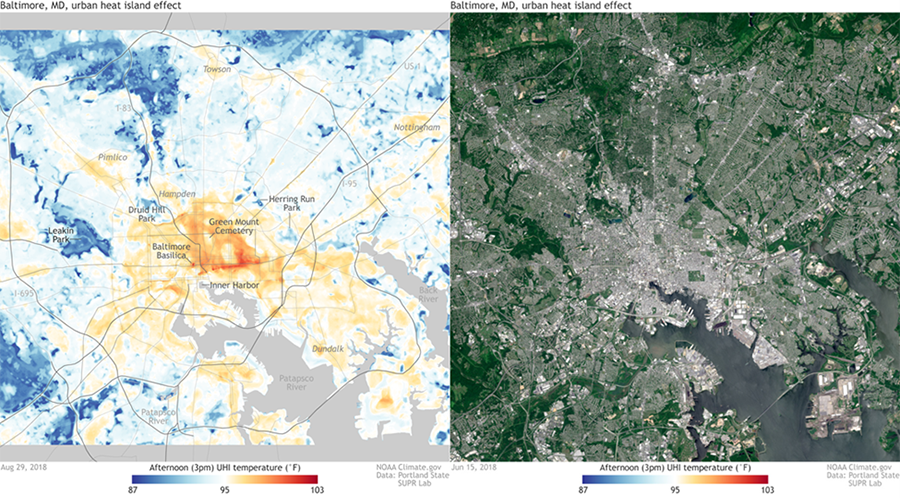
One of the consistent ways that hardscape influences urban climate is by making urban areas significantly warmer than surrounding rural areas, a phenomenon known as the urban heat island effect. Hardscapes, particularly dark-colored ones like asphalt, are generally a bit better at absorbing and storing solar radiation than vegetated landscapes. In addition, evapotranspiration is a powerful cooling mechanism that quickly dissipates much of the solar energy that vegetation does absorb. In contrast, hardscapes more slowly release the shortwave solar radiation they absorb during the day as longwave radiation (heat). On top of that, many of the machines of urban living, like air conditioning, add a bit more heat to the air in urban areas. The net result is that, averaged over the year, a modest sized city of 1 million people is about 1°C to 3°C warmer than the surrounding landscape.22 The urban heat island effect is most pronounced in the late afternoon and early night as cities sluggishly cool relative to the surrounding landscape. The effect is more pronounced on clear and calm nights, which accentuate the cooling advantage vegetation has. During these peak times, urban areas can be as much as 10°C to 15°C warmer than surrounding rural areas.23
The urban heat island effect is most pronounced in the heavily hardscaped core of cities and generally declines as you head out into the country. Baltimore’s temperature pattern is a good example (Fig. 8.7). But don’t let that give you the impression that the effect is isolated. Almost every bit of hardscape elevates temperature to some degree, and we have created an intricate network of elevated temperature that parallels the network of urban sprawl (see Fig. 3.16B). The elevated temperatures also influence other regional climate patterns that can stretch beyond urban areas. For example, locations 30–60 km downwind of several major US cities have an average of 28% greater rainfall compared to upwind locations, and some locations receive as much as 51% more rain.24 One likely cause of this is that the urban heat island creates a column of warm, rising air that contributes to the formation of downwind thunderstorms. A range of other urban factors such as the production of aerosols and airflow instability caused by the physical obstruction of buildings could also be factors.25
The urban heat island effect also indirectly influences global climate by contributing to greenhouse gas emissions. As I mentioned above, most of our greenhouse gas emissions are produced in cities, and a considerable slice of those emissions are associated with air conditioning. In the United States, about 8% of residential energy consumption is used to power air conditioners.26 Globally, air conditioners and fans account for 20% of the electricity used in buildings and about 10% of total electricity consumption.27 This impressive use is poised to increase dramatically for a couple of reasons. Thankfully, more people in the world are beginning to be able to afford an air conditioner, which for the sick, old, and very young is more a lifesaving necessity than a luxury. But also, demand for cooling is increasing as a result of human-driven climate change. The number of days when temperatures exceed a threshold that makes air conditioning a necessity is expected to increase 25% globally by 2055.28 The urban heat island effect exacerbates this trend. During extreme warm periods, there can even be a positive feedback between the intensity of the heat wave and the urban heat island. During one particularly hot summer in 2012, the urban heat island of Athens, Greece, intensified the effect of heat waves by as much as 3.5°C.29 The combination of rising affordability and demand for air conditioning is expected to more than triple the energy used for air conditioning by 2050.30 And it is not simply the greenhouse gasses associated with the energy consumption that is a concern. The refrigerants used by air conditioners are powerful greenhouse gasses. For instance, one of the most common hydrofluorocarbon (HFC) refrigerants used in richer countries has a climate warming potential 1,300 times that of carbon dioxide.31 Air conditioning has created another climate feedback. As we move to cities and use air conditioning, we create urban heat islands and release greenhouse gasses that make us need to use more air conditioning.
The urban heat island has a range of complex effects on the biology of individual organisms as well as overall biodiversity patterns. These are similar to (and interact with) the effects that global climate change is causing (see Chap. 5), including inducing range shifts by making urban areas either less or more thermally suitable to species, shifting the phenology of life history events such as flowering or diapause, extending growing seasons, increasing water demand, and influencing the growth patterns of organisms. For example, the growing season for plants in the heavily hardscaped parts of Madison, Wisconsin, is an average of five days longer than that in the surrounding rural area. Plants in the heavily hardscaped areas leaf out and flower earlier than ones in less hardscaped areas.32 Animals living in middle- and high-latitude cities also often have advanced timing of life history compared to their country cousins. For instance, acorn ants (Temnothorax curvispinosus) living in several midwestern US cities reproduce roughly a month earlier than acorn ants living in nearby rural areas.33
We have an overall poor understanding of the biological consequences of the urban heat island. One complication is related to the microclimate complexity of urban areas. For instance, organisms living in a large city park might experience a similar thermal environment to that of a more rural area. We also don’t have a good understanding of how the urban heat island is interacting with global climate change to influence organisms. In some cases, the effects of the urban heat island might provide a present-day glimpse of how global climate change might influence organisms more broadly in the future. One study found that plants in US cities started their growing season an average of six days earlier than plants in adjacent rural areas.34 The study also found that the overall relationship between temperature and the start of the growing season was weaker in cities than in rural areas. One reason might be related to winter dormancy. In temperate regions, many plants go dormant at the end of fall and then break dormancy when temperatures pass a certain threshold in the spring. To complete that process smoothly, plants need to be exposed to low chilling temperatures for a certain length of time. It may be that it now never gets cold enough for long enough in many US cities for plants to enter dormancy, and that disrupts the normally strong association between rising spring temperature and bud burst. That disruption could become more widespread—even in rural areas—as a result of global climate change. But the urban heat island and global climate change also sometimes affect organisms differently. For example, dragonflies and damselflies (Odonata) mostly don’t show any phenological shifts caused by the urban heat island. But the timing of their flight patterns has advanced significantly over the past few decades as a result of greenhouse-gas-driven climate change.35
Hydrology
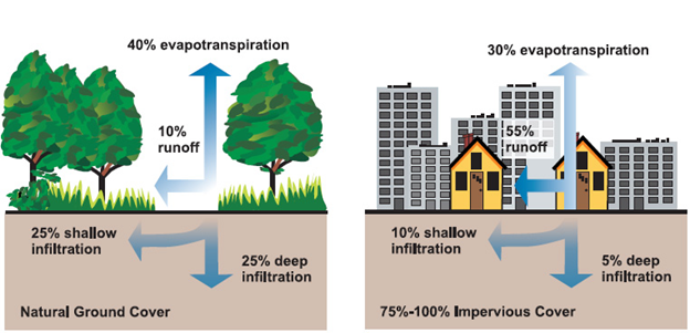
Water flows through urban areas in a fundamentally different way than it flows through vegetated landscapes. Broadly, when rain falls on vegetation, about half of it gets absorbed by the soil or percolates into deep aquifers, about 40% evaporates or is transpired by plants, and about 10% forms surface runoff. In a heavily hardscaped area, the pattern is reversed. Only about 15% of precipitation gets absorbed by soil, about 30% evapotranspirates, and a whopping 55% forms runoff (Fig. 8.8). This difference has multiple consequences.
All that runoff would chronically flood our living spaces if we did not channel it into an elaborate stormwater management system. The designs of these systems have changed over the years, particularly recently (see Section 8.5), but most are still oriented around the principle of diverting the runoff away from our built environment as quickly as possible. As a result, a good rainstorm acts like a cleansing power scrub for the city, washing away its accumulated grime and detritus. In many cities, the heavily polluted water gets unceremoniously dumped into rivers and oceans. In others, much of the stormwater gets combined with sewage waste from toilets and other wastewater streams, then sent to water treatment plants before being discharged. When it was introduced in the mid-1800s, these combined sewer system designs were meant to reduce pollution. As cities grew and became increasingly dominated by impervious hardscape, however, the capacity of their combined sewers was frequently overwhelmed by long or intense rainstorms. When this happens, an even dirtier cocktail of feces, pathogens, pharmaceuticals, pesticides, household chemicals, caffeine, heavy metals, oil, plastics, and nearly anything else you can think of gets belched out into rivers and coastal marine waters. These combined sewer overflows (CSOs), as they are somewhat euphemistically called, as well as stormwater runoff in general, have become major sources of aquatic pollution.36 This is a particularly important pathway for novel chemical pollutants such as pharmaceuticals and plastics, about which the biological impacts are not well understood.37
In addition to being laden with the detritus of modern life, urban runoff picks up a considerable amount of heat from the urban heat island. This heat is itself a damaging pollutant in many aquatic environments. Urbanization has been one important factor elevating stream temperatures and degrading aquatic habitat quality around the world. The impact has been particularly strong in cool temperate climates where many of the aquatic species have narrow (mostly cool) temperature requirements. For example, salmon habitat across the US Pacific Northwest has been degraded by elevated stream temperatures, partly caused by urbanization.38
Light
Another way we shape urban environments is with artificial light. The impact of artificial light on human society as well as the ecology of the planet is profound, although we often don’t appreciate this until there is a power outage. Night for most of us is now not dark but rather an artificial twilight of outdoor lighting, reading lamps, and the glow from smartphones. More than 80% of the world population now lives in light-polluted nights; in heavily urbanized regions such as the United States, it is more than 99%. More than one-third of us can’t see the Milky Way because of light pollution.39
There are three major ways all of this light affects organisms: (1) by disrupting spatial orientation and movement, (2) by disrupting a sense of time, and (3) by disrupting physiological processes.
Disrupting Spatial Orientation and Movement
Artificial lights can spatially disorient organisms, often those that use natural sources of light such as the stars and moon to navigate. Moths and other flying insects are probably the most visible example. I say “probably” because we still are not exactly sure how nocturnal insects navigate or why they are attracted to artificial light. But the attraction is often fatal, either from getting killed by the light directly (e.g., a candle flame), dying from exhaustion after fruitlessly circling a light source, or getting picked off by predators like bats that benefit from the insect aggregation. Exact numbers of the death toll are elusive, but it must be large enough to be a strong form of selection because moths living in urban areas have evolved to be less attracted to artificial light.40 Another notable example of light disorientation affects migrating birds. Although we don’t think of most birds as being particularly nocturnal, migratory birds do most of their flying at night, perhaps to avoid pesky visual predators like hawks. It seems that birds navigate at night using an internal magnetic compass combined with celestial navigation. Artificial lights muck up this exquisitely evolved system. Many birds are directly killed by colliding with lighted structures. An estimated 6.6 million birds are killed by navigating just into lighted communication towers in the United States alone.41 Estimates of bird deaths from buildings in general—including daytime collisions caused by disorienting reflections from windows—are immense. Somewhere between 381 million to 1 billion birds die annually in collisions with buildings in the United States and Canada.4243 The global death toll from collisions with all lighted structures must be immense.
Artificial lights also get birds lost or needlessly divert them. This confusion is now a chronic energetic drain on birds that make arduous migrations. The major migratory pathways for the world’s birds go through regions with the highest levels of light pollution.44 An inadvertent view into the migration and the effect that artificial lights can have on it comes from the annual commemoration of the September 11th attacks in New York City. The National September 11 Memorial and Museum has an annual Tribute in Light ceremony that shines powerful lights skyward in a moving tribute. The ceremony occurs right at the peak of the fall migration, and thousands of birds veer off from their migration to circle the lights in confusion.45 Check out the video in the Additional Resources. In this case, the solution has been to monitor the birds that are trapped in the holding pattern, and when numbers reach a certain threshold, the commemorative lights are turned off for a few minutes to let the accumulated birds go on their way. Similarly mindful tweaks to how we light our urban environment could be an even bigger help to migratory birds. Chicago is another city that sites in the migratory path of birds. McCormick Place Lakeside Center, a particularly large building, sits in a particularly bad spot along the edge of Lake Michigan. More than 40,000 dead birds have been recovered from McCormick Place between 1978 and 2020. One study estimated that halving the number of lighted windows in the building during the spring and fall migration periods could reduce bird deaths by 60%.46
Artificial light influences the movement patterns of other organisms in a variety of ways. Examples include beach mice that avoid foraging on lighted beaches.47 bats that are forced to take longer commutes between their roosts and foraging grounds to avoid lights,48 and spiders that are attracted to the abnormally high abundance of flying insects around artificially lighted streams.49 Even organisms that live entirely in the marine environment are affected. For example, marine zooplankton undertake perhaps the greatest daily migration of biomass on the planet. During the day, many zooplankton hang out in relatively deep and dim waters where they find a refuge from visual hunting predators. At night, they migrate up to shallow water to feed on phytoplankton. Artificial lighting has been shown to dramatically suppress this movement.50 These results come from small, local patches of ocean around boats and research platforms, but because light pollution affects large stretches of coastline, its impact on zooplankton movement could be widespread.
Disrupting a Sense of Time
Artificial light also confuses an organism’s sense of time. Life is metered out in the fundamental rhythm of day and night. The artificial blurring of day and night can therefore affect the basic things organisms do, like eat, sleep, and mate. For example, many songbirds dramatically start singing at dawn (the dawn chorus), continue with varying levels of intensity throughout the day, and then stop singing at night. But songbirds living in areas with artificial light have extended their singing period—either by starting earlier or ending later.51 City-dwelling blackbirds, for instance, start calling up to five hours earlier than their country cousins.52 When I lived in Los Angeles, a northern mockingbird (Mimus polyglottos) liked to perch next to my bedroom window and serenade me with a near-constant barrage of mimicked scrub jay calls, truck back-up signals, and car alarms that lasted nearly the entire night. Perhaps exhausted by the effort, it usually stopped singing right after dawn—the time I needed to wake up. Birdsong is only one of the many animal behaviors that artificial light has been shown to influence. Studies from across a range of species have shown that artificial light can disrupt sleep patterns, cause usually diurnal predators to extend their hunting into the night, cause usually nocturnal prey species to spend more of their nighttime avoiding predators instead of feeding, alter spatial foraging patterns, and disrupt mating behavior.53
Disrupting Physiological Processes
Many physiological processes are influenced directly and indirectly by day-night patterns. These include processes whose timing is based on light cues such as autumnal leaf drop in many plants and the seasonal timing of mating in many animals. In addition, many processes run on internal circadian clocks that have roughly 24-hour cycles. These cycles run autonomously, but like an old-fashioned wind-up clock, their timing can wander unless they are periodically reset in reference to an external light cue. Artificial lighting can cause the timing of processes paced by circadian clocks to get out of sync with when organisms actually need them to happen. It is like forgetting to turn a clock back at the end of daylight savings time and showing up an hour early for your first class—only chronically day after day. Perhaps not surprisingly, we are accumulating evidence that these disruptions can have a wide range of negative effects. For example, humans using electronic devices such as tablets at night have suppressed levels of the sleep-promoting hormone melatonin, making it harder to fall asleep. Once they do fall asleep, the sleep is disrupted in various ways so that they end up groggy and less alert the following morning.54 Artificial light has been found to alter a range of hormonally mediated processes (including sleep) in other animals.55 The physiology of plants is also affected. For instance, growers of greenhouse tomatoes must make careful use of artificial light. If the artificial day length gets too long, it can disrupt the synchrony between processes that are set using the tomato’s internal circadian clock and other process that are more directly affected by external light cues. Tomatoes that don’t get enough periods of darkness experience severe leaf damage and can even die.56
The range of effects that night lighting has on individual organisms can ripple throughout food webs and ecosystems in complex ways. One example of this comes from an experiment conducted using grassland mesocosms that were exposed to artificial light during the night at levels typically found along lighted roadways.57 In the night-light treatments, visual soil predators were more active (or perhaps more efficient), which significantly reduced the abundance of slugs, an important generalist herbivore in the system. For reasons that are not clear, the night lighting also significantly reduced the abundance and flowering of legumes. This in turn reduced the abundance of a legume specialist aphid species. These data give a hint that the basic structure and organization of many ecosystems are shaped at least in part by the artificial light we impose on them.
Sound
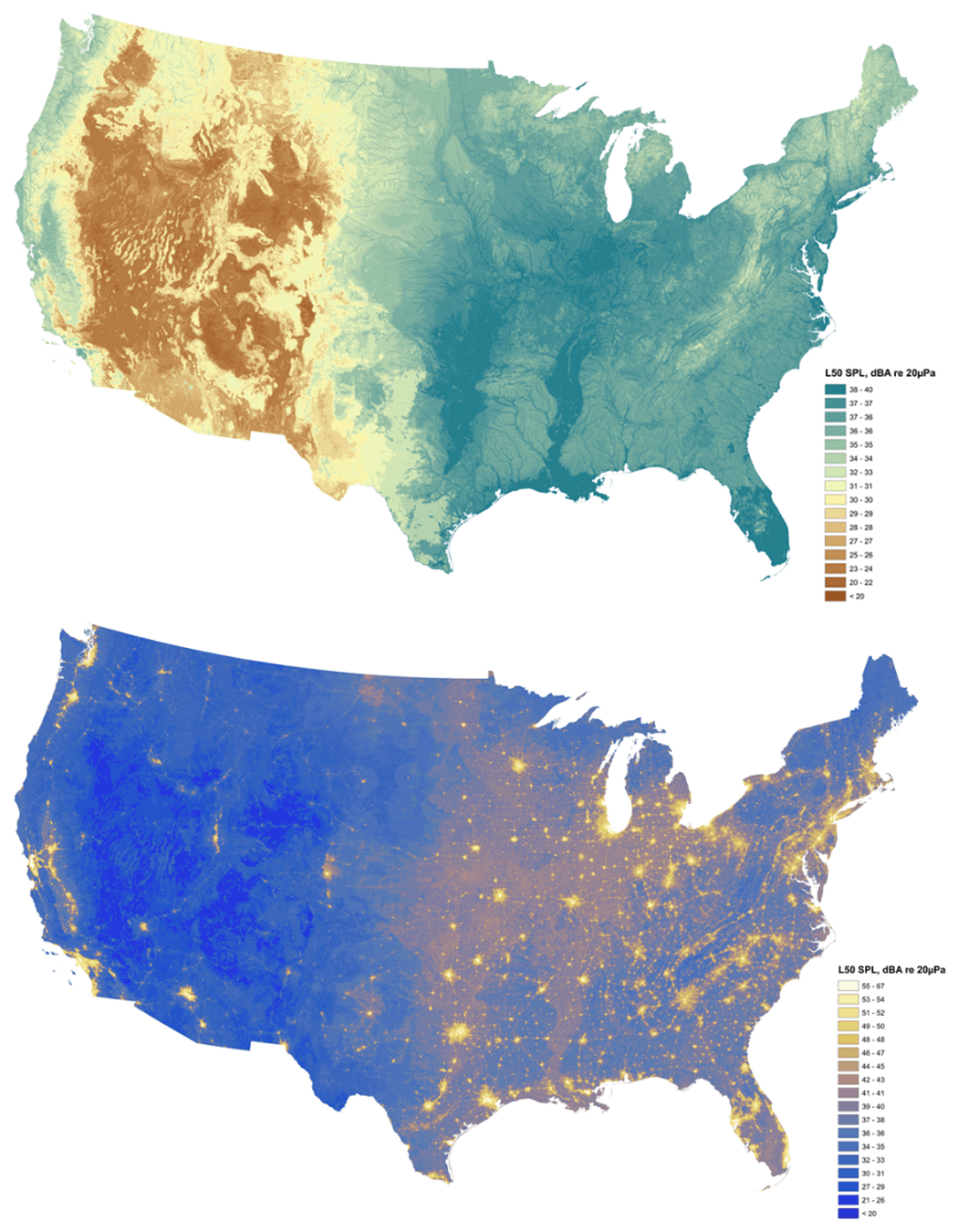
Earth has never been silent. The insistently calling mockingbird outside my bedroom window is just one example of Earth’s diverse biological sounds. Other natural sounds can be even louder, such as the 1883 eruption of Krakatoa that was reportedly heard 3,600 km away in Alice Springs, Australia.58 Into this natural soundscape we have added a cacophony of new sounds, largely since agro-industrialization. The noisy list is long: road traffic, airplanes, ship traffic, trains, industrial machinery, air conditioning, leaf blowers, a KISS concert, to name a few. These new sounds come in a variety of wavelengths, frequencies, amplitudes, durations, and times of the day, much of which are different than the natural sounds the planet has evolved with in the past. The new noise is chronic and pervasive. Just as nighttime is no longer dark, most of the planet now rarely experiences moments of relative quiet, let alone silence. While the sound reaches a crescendo in cities, human-generated sound also filters into rural and comparatively wild places (Fig. 8.9). Today, 63% of the protected areas in the United States (e.g., national parks, national forests) are twice as loud as their natural background noise level as a result of urbanized sound. Even worse, 12% of the protected areas are 10 times louder.59 Similar to artificial light, all the added sound is affecting the ecology of the planet in ways that we are just starting to document and understand.
One important effect is simply that all the added sound is making it difficult for organisms to hear each other over the racket. This is particularly important for species that use aural communication to find and maintain mates, structure their societies, signal dangers, and regulate resource competition. Urban populations of some of these species have altered the acoustic characteristics of their calls in order to be better heard in the urban soundscape. For instance, the sound associated with car traffic and machines is dominated by low frequencies. Many birds also have relatively low-frequency calls, making it difficult to compete against the wall of human-made sound. In response, urban birds often have higher-pitched (higher-frequency) calls relative to their rural counterparts.60 This high-pitched urban dialect stands out more amid the low-frequency rumble of cities. Birds and other organisms can shift calls in other ways. Common blackbirds (Turdus merula) living around the Madrid-Barajas Airport in Spain don’t use higher-pitched calls, but they use the louder part of their two-part song more often than forest populations. The airport birds sing earlier in the day (before the airport gets busy) compared to nearby forest birds.61 From the previous section on the effects of artificial light, you might wonder if that early singing is a result of light pollution, not sound. Sierro et al. (2017) wondered that as well and showed that the advanced singing only happens during winter and early spring when the dawn chorus coincides with the 7:00 a.m. start of flight operations. Later in the year, when the dawn chorus occurs before 7:00 a.m., airport and forest blackbird populations start singing at the same time.
It is not just communication between mates and rivals that noise disrupts. Sound conveys a lot of other environmental information, such as the location of prey or the presence of a dangerous predator. Noise can obscure these cues. For instance, traffic noise has been shown to reduce the hunting efficiency of aural predators such as bats and owls.62 For prey, noise can also distract attention away from approaching predators. This is the case for Caribbean hermit crabs (Coenobita clypeatus). Researchers were able to get much closer to the crabs (simulating a stalking predator) when they played recorded motorboat noise. It doesn’t seem that the motorboat noise was masking the sound of the approaching researchers. The researchers were able to get equally close no matter if they approached noisily or quietly. In addition, the researchers could get close when they flashed lights instead of playing motorboat noise. This suggests that the motorboat noise was distracting the crabs from being vigilant, not preventing them from hearing approaching predators.
We don’t know what the crabs found so distracting about the motorboat noise. It could simply be that, like many of us, they were annoyed by the racket disturbing their beach. Indeed, a range of animals seem to get particularly annoyed, alarmed, or otherwise put off by urban sounds. Sometimes this results in animals avoiding noisy areas. Daubenton’s bats (Myotis daubentonii), for instance, avoid foraging in areas where researchers played recorded traffic noise. The bats even avoided the areas when the traffic sounds did not overlap (and thus mask) the echolocation frequency signatures of the bat’s prey, indicating that the bats just didn’t like the noise in general even if it did not interfere with their prey-capturing ability.63 Avoidance seems to be a common response to urban noise, and a number of studies have documented reduced species richness in noisy areas.64 But for many organisms, avoiding noise is increasingly not an option, and there is growing evidence that chronic exposure to urban noise has a range of mostly detrimental physiological effects. The most comprehensive data come from ourselves. Studies have linked chronic noise exposure to impaired sleep patterns, elevated levels of stress-related hormones, high blood pressure, heart disease, tinnitus, reduced cognitive performance in children, and a range of psychological ailments such as anxiety and depression.65 Noise effects on human health are so pervasive that the World Health Organization estimates that in Europe alone, at least 1 million healthy life years are lost each year because of noise pollution.66 In contrast, natural sounds like running water or birdcalls seem to have the opposite effect, fostering a broad physiological shift from sympathetic (fight or flight) responses to parasympathetic (rest and digest or feed and breed) responses.67 Studies have found similar effects in other animals. For instance, the sound of shipping traffic and other industrial noise elevates the physiological stress levels of many marine organisms including invertebrates, fishes, birds, and mammals.68
8.3 Urban Biodiversity
Section 8.3: Urban Biodiversity
Not surprisingly, the urban physical environment creates unique patterns of biodiversity. We are just beginning to describe and understand this urban biodiversity. In some ways, we understand the biology of remote and insanely complex habitats like tropical forests and coral reefs better than the habitats where most of us live and interact with the natural world. This is in part because we have often dismissed these habitats as uninteresting concrete jungles inhabited by a handful of boring, ubiquitous species. This view is beginning to change, and we are realizing that urban habitats are biologically fascinating. Urban biodiversity can be grouped into several broad categories.
Domesticated Landscapes
Much of urban biodiversity is domesticated (see Section 6.4). The vegetation in urban landscapes is a prime example. Most urban vegetation is composed of species and varieties that we have specifically selected or bred. We organize these selections into planned associations and vegetation types: lawns, landscaping, gardens, street trees, parks, urban farms, and houseplants. We then spend a great deal of time and other resources caring for and maintaining our creations. Despite the attention and resources we invest in them, not to mention the joy we derive from them, we tend to ignore or even actively dismiss the ecological characteristics of our created urban landscapes. Understandably, we have tended to view them more as parts of our constructed human world than as parts of the natural one. But we are beginning to better appreciate their unique ecological characteristics and functions. A few broad characteristics have so far emerged.
They Have High but Homogenized Plant Species Richness
Urban vegetation can be surprisingly diverse—at least in terms of some aspects of biodiversity. Studies have consistently found that patches of urban vegetation tend to be considerably more species rich than adjacent patches of natural habitats.69 This is in sharp contrast to agricultural landscapes that tend to be much less species rich than adjacent uncultivated areas. This difference seems to reflect the fact that, unlike farmers, the managers of urban landscapes have a much more variable range of goals and management styles. This is even the case in North America where the turf grass lawn seems to define our image of urban vegetation.70 A stroll down nearly any suburban street will indeed take you past well-manicured turf grass lawns, but also a kaleidoscope of plants from around the world arranged into an infinite number of ways, from formal French gardens, to naturalistic native habitat designs, to botanically exotic horticultural showcases. There is some evidence that our landscape designs reflect the fact that we prefer more diverse landscapes, although we often focus not so much on species richness as on other diversity components such as structural complexity.71
Our diverse tastes don’t translate across all biodiversity metrics or across all scales, however. As described in Chapter 6 we have developed a global trade in ornamental plants. In many instances, most of the species that are available for sale at nurseries are not native to the local region. For example, only about 15% of the plants sold by Florida nurseries in 2019 were native to Florida.72 One consequence is that a similar list of species tends to be offered for sale at nurseries and grown in landscapes across large regions and even around the world. Gardening styles, trends, and fads also increasingly spread globally. Just as in agroecosystems, management tools such as irrigation allow us to implement designs using similar sets of species no matter what the local conditions are. The net result is that although urban floras tend to be species rich, they also tend to be relatively similar to each other compared to the natural floras in their respective regions (see Fig. 6.7).
Their Biodiversity Patterns Are Strongly Influenced by Human Social Factors
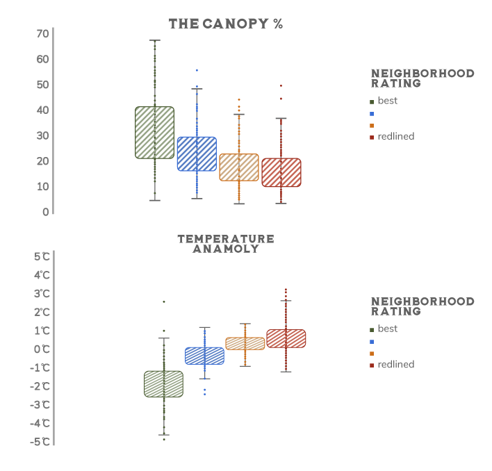
Because we design and manage them, the biodiversity patterns of our domesticated urban landscapes are as much influenced by socioeconomic factors as they are by environmental characteristics such as climate or soil type. One important factor is wealth. In cities around the world, wealthier neighborhoods have greater vegetation cover and plant diversity than poorer neighborhoods—a phenomenon that has been called the luxury effect.73 This effect partly reflects the usual privileges that come with wealth, such as a greater ability to afford the higher rents and home prices found in greener neighborhoods, more disposable income to spend on home gardens, and greater political influence to drive the creation and maintenance of public green space in their neighborhood. Another important cause is systemic racism and classism.74 This can play out in a number of locally nuanced ways. One example comes from the United States. In the 1930s, the federal government launched a program to help refinance home mortgages at discounted rates in an effort to prevent foreclosures during the Great Depression. As part of the program, they rated neighborhoods in terms of their perceived safety for lenders: from best to hazardous. The federal Home Owners’ Loan Corporation made color-coded risk maps for cities, with the highest-risk neighborhoods in red. This program of redlining was fundamentally racist, as the assessment of real estate risk was largely based on the racial makeup of the community: black and immigrant-dominated communities were deemed high risk, while white US-born-dominated communities were deemed safe bets. Redlining has profoundly shaped the social and economic trajectories of people living in those communities ever since.75 It also has influenced current biodiversity patterns in US cities. For instance, formerly redlined neighborhoods have considerably less green space and tree cover than neighborhoods that rated as best.7677 As a result, residents of these communities have significantly less access to the ecosystem services associated with green space. For instance, residents of formerly redlined neighborhoods in eight California cities have 2.4 times more asthma-related emergency room visits than residents of non-redlined neighborhoods. One likely cause is that redlined areas have higher levels of air pollution related to their reduced green space and greater concentration of the pollution-generating parts of hardscape such as roads.78 Across the United States, residents of formerly redlined neighborhoods also suffer considerably more from the urban heat island than do residents of non-redlined neighborhoods (Fig. 8.10).
We also express our cultural identity or signal our social position through urban domesticated landscapes. In South Africa, for example, members of the Batswana (Tswana) ethnic group traditionally have home landscapes that are composed mostly of native food and medicinal plants. But people (including many Batswana) living in newer middle-class neighborhoods tend to have landscapes that contain many ornamental species that are part of the global horticultural trade and that wouldn’t look out of place in nearly any middle-class neighborhood around the world.79 In Southern California, many people in immigrant communities design their gardens to provide culturally specific food, traditional medicine, or simply as reminders of their ancestral landscapes.80
Their Biodiversity Patterns Are Strongly Influenced by Our Management
As in our agroecosystems, we shape biodiversity patterns in our urban domesticated landscapes by altering physical conditions, manipulating the composition of species, and diverting flows of energy and resources. In addition, there is considerable variation in the use of practices as well as what the net effect on biodiversity is—perhaps even more so. But we have evidence for a few general relationships that mirror the patterns discussed for agroecosystem in Chapter 7.8182
The intensive use of resource inputs (nutrients and irrigation) as well as chemical pest management generally lowers biodiversity in urban domesticated landscapes. For example, in Paris, France, lawns that are not treated with pesticides have higher plant species richness, a greater number of rare species, and more insect-pollinated species than pesticide-treated lawns.83 Similarly, the plant diversity of lawns in Xi’an, China, is negatively associated with the frequency of chemical fertilizer applications.84 Multiple practices often interact, and the effects can ripple through interaction webs. For instance, the use of both insecticides and herbicides reduces the abundance of bumblebees and butterflies in French gardens. The insecticides directly affect the insects, while the herbicides indirectly affect them by reducing the abundance and diversity floral resources.85
The French garden example illustrates that the plant diversity of urban domesticated landscapes has a strong influence on the diversity of other groups such as insects. Another example comes from Zurich, Switzerland. In Zurich, gardens that have high plant species diversity have a high diversity of soil-dwelling organisms as well as high levels of multiple soil processes mediated by those organisms, such as decomposition and soil organic matter mineralization.86 We alter plant-animal relationships in urban domesticated landscapes through the choice of plants that we use (see above), through plant domestication (see below), and through management practices. The management practices include not only the use of resource inputs and herbicides, but also practices such as mowing that affect disturbance patterns. For example, suburban lawns in Springfield, Massachusetts, that are mowed every three weeks have 2.5 times more flowers, more bees, and greater bee species richness than lawns that are mown weekly.87
Urban landscape designs that involve more structural complexity also tend to support higher levels of animal diversity—in much the same way that more structurally complex agroforestry systems do (see Fig. 7.3). For instance, in the parks and gardens of Melbourne, Australia, bird species richness increases with increasing volume of understory vegetation, while bat species richness is positively associated with the density of big trees.88 The different habitat requirements of bats and birds illustrate that our management practices can have different effects on different taxa or on different aspects of biodiversity. For example, mulching significantly increases the density and species richness of garden spiders,89 but it reduces the abundance of pollinators such as bees.90 Mulch improves habitat for a range of soil organisms that the spiders feed on, but mulch negatively effects pollinators because many pollinator species need bare soil for their nest sites.
They Have Unique Traits and Interactions
Beyond diversity itself, the species composition of our domesticated urban landscapes is also markedly different from neighboring non-domesticated landscapes. As mentioned above, urban domesticated landscapes are dominated by assemblages of plant species that are mostly non-native to the region and that are shared through the global nursery trade. As a result, the domesticated landscapes of even distant cities can share far more species in common than their respective non-domesticated landscapes.91 In addition, the functional trait composition of domesticated floras differs from natural vegetation. The horticultural processes of selecting, breeding, and mass rearing of ornamental plants create unique characteristics. Most nursery plants are produced through asexual propagation so that plants sold at nurseries around the world are nearly genetically identical. Many commercially grown ornamental species are selections made from a small subset of the wild genetic diversity from which they are drawn. These selections can reflect particularly oddball or rare phenotypes. Breeding can also create novel traits such as new flower colors or different leaf shapes.
Much of our manipulation of ornamental plants is aimed at producing traits that we find interesting and attractive, but these can also be less attractive or confusing to other species. In turn, that can disrupt important plant-animal relationships such as pollination. For example, a desirable trait for ornamental varieties is double flowering, where some or all of the stamens in a flower are replaced by petals. This creates bigger and fancier flowers, but it can also degrade their value to pollinators by reducing the amount, quality, or accessibility of pollen and nectar.92 Other common traits favored in the nursery trade such as sterility, novel flower color, novel leaf shape and color, and compact growth form can alter not only pollinator resources but also the value of the cultivars as a food source for insect herbivores. One study found that ornamental cultivars whose leaf color had been changed from the wild-type green to red or purple were less attractive to leaf-feeding insects.93 But there hasn’t yet been a lot of work describing how ornamental cultivars vary in their suitability to insect pollinators and herbivores. The handful of studies that we do have suggest that while there may be a tendency for native cultivars to be less suitable for pollinators than their corresponding wild type, there is a considerable amount of variation among taxa.
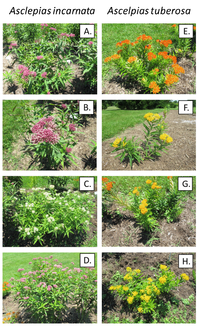
One study evaluated insect pollinator preference for wild type or cultivar forms in fourteen species of native perennials. In nine species, pollinators preferred the wild type, in one species they preferred the cultivar form, and there was no preference for the wild type or cultivar in four species.94 In some cases, cultivars are capable of providing a broad range of resources that are comparable to wild type forms. For example, milkweeds (Asclepias spp.) are the obligate larvae host for the monarch butterfly (Danaus plexippus). Monarch butterflies have been in precipitous decline over the past several decades, and one part of conservation efforts has been to increase the abundance of milkweed populations throughout North America.95 There are many species of milkweed whose distributions vary across North America as well as a wide range of ornamental cultivars that have been developed that could differ in their suitability as monarch hosts (Fig. 8.11). But a study that evaluated the host suitability of different cultivars found that cultivars were colonized by monarchs to the same extent as wild types, and although there were some differences among the cultivars in terms of herbivore defense traits, all cultivars were as suitable as wild types in supporting monarch larval growth. The cultivars were also equally attractive to bee species that use milkweed floral resources.96
Variability in habitat provisioning is also seen at the scale of whole assemblages of domesticated plants and across domesticated landscapes. In some cases, urban landscapes provide overall poorer habitat. For example, the reproductive success of Carolina chickadees (Poecile carolinensis) living in and around Washington, DC, is reduced by the presence of non-native woody plants in the yards they live in. Yards that are dominated by non-native plants have lower arthropod abundance than yards dominated by native species. Chickadees are insectivores, so the ones living in the non-native dominated yards have less food, which results in reduced nest success. The effect is so strong that only yards whose woody plants are at least 70% native can support viable chickadee populations.97 Herbivorous insects tend to be picky when it comes to the plants they feed on. A large proportion of them are specialized on a narrow set of host plant species. This is probably the main reason why the non-native and horticulturally manipulated species that dominate urban landscapes seem to be relatively poor habitat for many of them.
But in other cases, urban domesticated landscapes can provide valuable habitat, sometimes meeting the unique requirements of habitat specialists. Green roofs (see Section 8.5) in Switzerland provide habitat for a rich assemblage of ground beetles (Carabidae). While most of the beetles are widespread and common species, the roofs also support a few habitat specialists that require the unique combination of low vegetation cover, high temperatures, and windy conditions found on the green roofs. Four of these species are rare or endangered in Switzerland.98 The species that most commonly utilize urban domesticated landscapes are habitat generalists, however. These species have habitat needs that tend to be satisfied by many different plant species and genotypes. For example, many bee species are floral generalists that can access nectar from a range of different floral types. They tend to be more concerned about the overall abundance of nectar-producing flowers than about fine differences among species. As a result, even gardens and parks that are dominated by non-native plants can still support rich assemblages of bees as well as other insect pollinators.99 In New York City, community gardens support 54 bee species, 13% of the overall bee fauna found in the state of New York.100 In Germany, cities support a higher diversity of bees, and flowers have higher pollination rates than rural areas.101
In that German study, the reason for the greater urban bee diversity is not particularly clear. Urban and rural sites didn’t differ in their floral abundance or the amount of insect-friendly habitat such as weedy edges they had. One possibility is that urban areas provide more of the nesting habitat that many bee species require, such as bare soil for ground-nesting bees, dead wood for mason bees (Osmia spp.), and various nooks and crannies for bumblebees (Bombus spp.). Bees might also be particularly susceptible to agricultural management practices such as the intensive use of pesticides. In contrast to the bees, other groups of flying insects such as flies, butterflies, and moths were more diverse in rural areas than in German cities. Results such as these indicate that we still have a lot to learn about the ecological characteristics of urban domesticated landscapes. But they are distinctly different from natural settings and even agricultural landscapes.
Domesticated Animals
We share our urban environment with a diverse array of domesticated animals. In many parts of the world, pigs, chickens, goats, and even cattle provide important sources of food and income for urban residents. Urban livestock operations include the distribution networks that move rural livestock to urban consumers as well as small, fully integrated operations where the livestock are often raised a few feet from where they are consumed. Such intimate cohabitation has long fostered the evolution and transmission of zoonotic diseases—infectious diseases that are transmitted between species. Viral diseases provide many examples. The COVID-19 pandemic was caused by a coronavirus (SARS-CoV-2) that originated in another species and may have crossed into humans in a market that sold live animals in Wuhan, China.102 The 1918 influenza pandemic was caused by the H1N1 strain of influenza. Influenza A strains primarily infect birds, but they frequently cross over to mammals, creating particularly virulent forms when they do. In addition to the 1918 pandemic, several other pandemics have been spawned by influenza A species crossovers. Our cohabitation with poultry and pigs seems to have created a particularly effective pathway for the influenza A crossovers to happen.103 There is some evidence that urbanization is interacting with the other drivers of biodiversity change (see Chap. 6 in ways that enhance the epidemiological connection between humans, livestock, and wild animals. In Australia, for example, flying foxes (bats in the genus Pteropus) have become common urban visitors, and in many cases full-time residents. Their move to the city has been driven by the loss of their traditional forest habitats as well as the abundant supply of flower and fruit resources in the gardens of Australian cities. This puts the bats in much closer and more frequent contact with humans and our domesticated animals such as horses. This new cohabitation seems to be facilitating the transmission of the Hendra virus from bats into humans and horses. Hendra virus infections can be deadly for both humans and horses. Of the 14 known Hendra virus outbreaks, 10 have occurred near urbanized flying fox populations.104
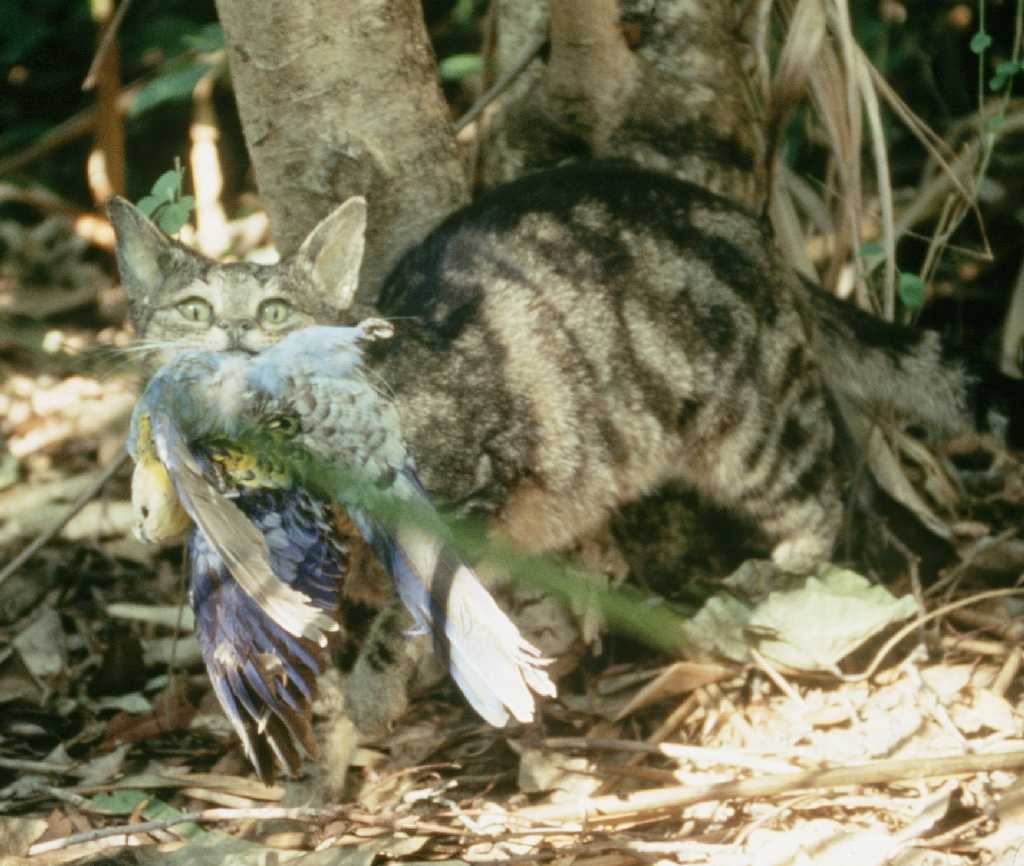
The other animals we live in intimate cohabitation with are pets. For many people, pets are the most direct and intense connection they have with the natural world. You might laugh at the idea that pets are even part of the natural world given how closely their lives intertwine with ours. We even seem to have bred (perhaps unconsciously) dogs to have facial muscles that allow them to better communicate with us nonverbally.105 The influence that pets exert on urban ecosystems is partly mediated through their association with us. For instance, a portion of the food that households consume and the wastes that they generate is due to pets.106 But pets also exert influences unique to their own ecological traits. Free-roaming domestic cats and dogs are important predators in urban areas as well as along the wildland-urban interface. Cats alone kill an estimated 1.3–4.0 billion birds and 6.3–22.3 billion mammals in the United States annually, making them the single largest way our activities directly kill birds, outranking other notable human-driven causes of mortality such as building collisions and pesticide poisoning.107 Worldwide, domestic cat predation has contributed to at least 63 vertebrate extinctions (mostly on isolated islands) as well as more widespread population declines and behavioral changes.108
Many of the animals exerting this influence are not what we would think of as pets exactly. They are feral, living out much of their lives roaming freely and independent of us (Fig. 8.12). But they aren’t exactly wild, either. Some people feed or otherwise help feral populations of cats and dogs, either out of affection or out of a belief that the populations provide benefits such as pest control. Our help allows these populations (and their impact) to be much larger and more consistent than they otherwise would be. Our affection for domestic cats and dogs also prevents us from effectively managing their populations; attempts to control feral cat populations are often met with stiff human opposition.109 Pampered pets aren’t innocent, either. In Australia, the per capita kill rate of roaming pet cats is 25% less than that of feral cats, perhaps reflecting their relative indifference and inexpert hunting skills. But pet cats live at much higher densities in urbanized areas. As a result, the overall predation rate of pets per square kilometer in the residential sections of Australian cities is 28–52 times greater than predation rates by feral cats in natural areas.110 Pets and feral animals also have a range of more indirect effects on wildlife, such as facilitating the transmission of zoonotic diseases, hybridizing with non-domesticated species, and causing widespread fear simply by their presence, which disrupts behaviors such as foraging and mating.111
Exploiters and Adapters
Many species of plants and animals have adjusted to take advantage of or to tolerate urban environments. The ones we probably think of most are those we consider pests or that make us sick. Our close association with many of these species goes back to the origins of human settlement, and both they and we have spread around the globe together in an uneasy traveling party. Examples include bed bugs (Cimex lectularius), which have been causing us itchy nights since at least the reign of King Tutankhamun in Egypt,112 and brown rats (Rattus norvegicus), which hitched a ride with us around the world as we stitched together urban centers with trade and transportation networks.113
But the list of species that use urban habitats goes well beyond such ancient bedfellows. Several processes continue to attract species into urban spaces. First, urban habitats can provide a range of resources or environmental conditions that match the habitat needs of many species. A big attracting resource is food such as the prodigious amount of human food waste that attracts many animals,114 the light-pollution-driven aggregations of flying insects that attract predators such as bats,115 the flower and fruit resources in our domesticated landscapes that attract animals such as pollinators,116 and our domesticated animals that attract carnivores.117 Greater food availability can make cities attractive places even for species that are not strictly urban specialists. For example, peregrine falcons (Falco peregrinus) living in the cities of Great Britain have access to far more prey than rural peregrines; as a consequence, urban populations have greater nesting success than rural ones.118 Urban environments can also meet the physical habitat requirements of many species. In fact, the high level of physical habitat complexity found in cities may create favorable conditions for a range of different types of species. The rare beetle species supported by green roofs in Switzerland mentioned above are a good example. Many plants also find suitable habitat in urban spaces. For instance, the urban parts of New South Wales, Australia, support 136 native plant species that inhabit a diverse array of uniquely urban habitats such as railway embankments and suburban lawns.119
In some cases, species are not so much attracted to cities as they are pushed toward them. Many species are forced into using urban habitats because of degradation or loss of their original habitat. An example is the deforestation that contributed to the increased urban abundance of Australia flying foxes mentioned above. The spreading sprawl of the wildland-urban interface also forces species to use (or at least frequently pass through) urban habitats. The mountain lions of Southern California are an example (see Figs. 8.4 and 8.6). The consequences of the forced use of habitat varies for each species and even for each urban context. As I describe above, Southern California mountain lions have largely suffered from the urban sprawl that has encircled them. But the picture is a little different for another large cat. Indian leopards (Panthera pardus fusca) have been facing a long decline because of hunting and habitat destruction and are now found in only about 28% of their historic range. Their current range includes the burgeoning city of Mumbai, which supports the world’s highest density of leopards. Mumbai leopards seem to be doing relatively well because they have access to lots of prey, including livestock and feral dogs. The high density of leopards in Mumbai has resulted in conflicts with humans, which have unfortunately resulted in death and injury for both humans and leopards. But leopards also provide an important service. By keeping the feral dog population in check, leopards significantly reduce human deaths from dog bites and rabies.120
Organisms adjust to urban environments behaviorally, physiologically, and evolutionarily. Often all three forces are at play, and it can be difficult to disentangle their relative role in specific cases. On the behavioral side of things, being smart seems to be a particularly valuable trait. Animals can use their intelligence and problem-solving skills to take advantage of opportunities and to avoid dangers in urban environments. Coyotes (Canis latrans) are an archetype of intelligent adaptability. Every major city in the continental United States has been colonized by coyotes in part because of their inquisitiveness, unflappability in the face of novel dangers, and their ability to learn (Fig. 8.13). Some form of these traits served coyotes well (and still do) in their ancestral habitat of arid grasslands and open woodlands, but they also provided coyotes with the behavioral flexibility to adjust to urban conditions. Urban coyotes are bolder and more exploratory than rural coyotes. That shift in behavior seems to have happened over several decades, and it could reflect the spread of socially transmitted learning,121 sort of like how hipster culture has spread in cities across the world.
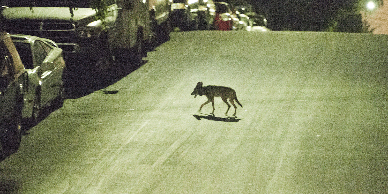
There are many examples of urban environments driving evolutionary change.122 In some cases, populations have evolved adaptations that help them in urban conditions. One example comes from urban populations of white clover (Trifolium repens). Many individual white clover plants possess an inherited trait that allows them to produce hydrogen cyanide, an effective defense against herbivores. But the trait comes with a trade-off: individuals with the cyanide trait are more susceptible to frost damage. A bit counterintuitively (given the urban heat island effect), white clover living in the cities of Ontario, Canada, face a harsher winter than their relatives in rural areas because urban areas have significantly less insulating snow cover than rural areas. Clover and other low-growing plants therefore get exposed to much colder temperatures than their snow-blanketed relatives. The harsher conditions strongly select against individuals with the cyanide trait. This has produced a remarkably consistent decreasing cline in the frequency of the cyanide trait as you move from rural to urban areas across all of southern Ontario.123 There are many animal examples of adaptive evolution as well. In their original forest environments, Puerto Rican crested anoles (Anolis cristatellus) perch on tree trunks. But in urban environments, they must negotiate a range of different hard surfaces such as glass windows and metal fences. Also, urban habitats are more open than forests, which forces urban anoles to spend more time running on the round between perches instead of jumping between them. Urban anoles have adapted by evolving longer limbs, which allows them to speedily run across flat surfaces. They also have evolved more gripping scales on the underside of their toes, which help them better grip hardscapes.124
Not all urban evolutionary changes are adaptive. The sprawling and fragmented nature of urban habitat inhibits gene flow so that urban populations are often composed of many genetically distinct subpopulations. Brown rats living in Manhattan are divided into genetically distinct uptown and downtown subpopulations, possibly because they don’t like to cross midtown, which has fewer food resources.125
Organisms can adjust physiologically to environmental conditions, such as when climbers acclimatize to the low oxygen at high altitudes. Toads (Bufo bufo) living in urban areas provide an example. Urban toads have larger toxin glands and produce a more potent mix of chemical defenses than toads living in more natural areas. The changes seem to be driven by physiological responses to the environment, not by selection-driven evolution. When wild-caught urban toads are brought into the lab, their offspring revert to a less potent state. It is not exactly clear why or how urban toads adjust in this way. It could be that urban toads produce more defenses because they perceive greater predation risk from predators such as cats and dogs. The enhanced predator defenses could also be an unintended side effect from exposure to urban pollutants, many of which are known to interact with the chemical pathways the toads use to synthesize their defenses.126
Remnants and Old Timers
Some organisms living in urban environments do so more or less accidentally or by historical circumstance. These organisms don’t find urban environments all that beneficial, and they haven’t adjusted all that much (if at all) to the new urban conditions they find themselves in. They persist either because conditions in their immediate local environment are still favorable for them or because they are able to grudgingly tolerate the suboptimal conditions, at least for a while. Southern California populations of mountain lions perhaps fit better into this category than the exploiter and adapter category.
Because of their largely sedentary and often slow-paced nature, plants provide most of the best examples. Individual trees and shrubs can live for decades and even centuries as the landscapes around them transform from wildland to dense cities. In 2019, a roughly 600-year-old white oak (Quercus alba) in Salem, New Jersey, finally succumbed to the fate that awaits us all. It was already a mature tree in 1675 when local lore says the Quaker John Fenwick and chiefs of the Lenni-Lenape people signed a land deal under it.127 Back then, the whole region was a rural landscape. By the time the tree died, it found itself in the middle of one of the most urbanized regions on the planet: the web of urban sprawl connecting Philadelphia, Baltimore, and Washington, DC. Still, the tree had some lucky breaks that allowed it to survive when so many of its contemporaries did not. Salem sits in a remarkably rural remnant of the otherwise urban region. The Quakers have managed the church cemetery where the tree grew as open space since 1675, and it looks pretty much the same as it did back then—as long as you don’t let your gaze travel too far afield.
It is not just individuals that can become relics of the past. Whole chunks of vegetation and their associated interconnected communities of organisms can get caught up in the urban matrix. Many times, this happens on neglected or somehow forgotten bits of land. For instance, many diverse and functional wetland habitats exist in the accidental interstitial spaces of urban areas such as abandoned industrial zones.128 But in addition, civic leaders often intentionally preserve their remnant and adjacent patches as regions urbanize. Many of these remnants are managed as amalgams of domesticated and natural landscapes, but many have the explicit goal of preserving the nature that existed before the city. An example is Forest Park in Portland, Oregon, a 2,064-ha swath of forest just to the west of downtown. The park was formally dedicated in 1948, but it resulted from planning and land acquisitions that had begun in the 1860s when civic leaders lobbied to create a nature preserve for residents of the growing city. Urban preserves are often part of larger regional networks of conservation areas. These networks can be extensive and encompass nearly all of the remaining wildlands in a heavily urbanized region. The more than 60,703-ha Santa Monica Mountains National Recreation Area (home to some of the celebrity mountain lions of Los Angeles) is a great example. The recreation area contains a network of parks that preserve a majority of the Santa Monica Mountains and their adjacent beaches as open space.129 Remarkably, it does that while bisecting one of the most densely populated urban centers in the world (Fig. 8.4).
The remnant patches of a former wilder time, whether they be a single tree or a vast network of preserves, are not isolated from the effects of the urbanization that surrounds them. To varying degrees, they are influenced by the conditions and processes described in Sections 8.1 and 8.2. As a result, they are not exact copies of the vegetation or communities that existed before the city grew. For instance, many have a significantly altered species composition that includes many non-native species. They are examples of the unique ecosystems developing during the Anthropocene. I will describe these novel ecosystems, as they are often called, in more detail in Chapter 9.
8.4 Improving Resource Use Efficiency
Section 8.4: Improving Resource Use Efficiency
Much of the impact that urbanization exerts on the Earth System is related to the massive amounts of energy and other resources that flow to and through cities. Improving the resource use efficiency of urban areas is therefore an obvious way of reducing their environmental impact. In Chapter 7 I describe the general approach to developing efficiency metrics and improving the efficiency of agroecosystems (see Section 7.4). While it is a straightforward exercise to describe the main benefits and costs associated with agriculture (even if we take a broad view of what those benefits and costs are), things are a bit more complicated for urban ecosystems. For one, we are often uncertain about the benefits of urban ecosystems. Also, even residents of the same city can have opposing ideas about what the benefits are, as well as how they perceive costs and constraints. I will explore some of these complications in this section as well as in Section 8.5. But in broad terms, there are several approaches to improving the resource use efficiency of urban areas that fall into several main focal areas.
Resource Efficiency of Built Structures
Many of the resources we use in urban environments go toward constructing the urban environment itself (all that concrete and other materials), keeping the lights on, and controlling the climate of our living spaces. We are making big strides in reducing the per unit or per capita amount of resources needed to do those things through improved industrial processes, more efficient building techniques, more efficient machines and appliances, and more efficient architectural designs. Without those efficiency improvements, the steady and prodigious increase in resource use that has occurred over the Great Acceleration would have been even bigger. For example, from 1980 to 2010, the total global annual amount of energy we used to power residential buildings increased by about 65%; the increase was driven by growing population as well as by greater per capita demand for energy. The increased per capita demand partly came from more computers, smartphones, and Internet connections. But it also reflected fundamental improvements in people’s lives, such as families finally getting their home hooked up to the power grid or finally being able to afford an air conditioner or space heater. That increase in demand would have resulted in far greater total energy use if not for steady improvements in the energy efficiency of appliances and of homes themselves. In many regions, efficiency improvements kept the actual per capita use of energy for residential buildings unchanged even as the overall demand increased.130
We have also improved efficiency by reducing the environmental impact that building and managing our cities causes. For example, although the pace is slower than it needs to be, we have started to transition away from greenhouse-gas-producing energy sources. Other examples include emerging technologies aimed at reducing the CO2 emissions associated with cement production,131 developing new pavement materials that are permeable to stormwater,132 adjusting the spectral composition of artificial lighting to reduce the impact of light pollution,133 and the use of new building materials and designs to mitigate the urban heat island effect.134
Resource Efficiency of Domesticated Landscapes
It takes resources to create and maintain our urban domesticated landscapes. In 1976, John Falk published an ecosystem energy budget for a suburban lawn in Walnut Creek, California, similar to what the Odum brothers had done for the Enewetak coral reef (see Table 3.1). As part of his study, Falk calculated the energy inputs associated with managing the lawn (Table 8.1). Interestingly, Falk found that the California lawn generated about as much net primary production as midwestern cornfields and tall grass prairies. But the lawn also sucked in a lot of outside inputs such as irrigation water, fertilizer, fuel for the lawn mower, and human labor. The energy it took to do the yard work and to transport and manufacture the resources totaled 578 kcal/m2/year, an amount comparable to the energy inputs required to grow midwestern corn.135
CategoryManagement ActivityEnergy Input (kCal/year)
| What It Takes To Keep a 110-m2 Lawn in California | ||
|---|---|---|
| Raking | General | 1,988.7 |
| Irrigation | Labor | 781.4 |
| Water delivery | 140,792.7 | |
| Fertilizing | Labor | 100.8 |
| Manure | 1,800.9 | |
| Chemical fertilizer | 11,057.2 | |
| Lawn Mowing | Labor | 1,983.9 |
| Gasoline | 45,281.3 | |
| Reseeding | Labor | 23.8 |
| Seed | 1293.7 | |
| Miscellaneous Labor | General | 71.3 |
Values for more tangible resources such as water and nutrients are equally impressive. Depending on the climate, 40% to 70% of the water used by households in the United States goes to irrigate their landscapes.136 A survey of homeowners and lawn care companies in Baltimore County, Maryland, found that lawns receive an average of 98 kg N/ha/year,137 an amount only modestly less than the 157 kg N/ha/year recommended for commercially growing corn in the region.138 Just as in many agricultural landscapes, much of the applied nitrogen flows away. The majority of the nitrogen entering watersheds in St. Paul, Minnesota, comes from fertilizer applied to its landscapes, primarily residential lawns.139 We also use a lot of pesticides on urban landscapes; nearly 75% of US households use chemical pesticides (insecticides, herbicides, fungicides) on their landscapes.140 We don’t have many good direct estimates of exactly how much we apply, however. A few studies have found that bees foraging in urban landscapes received a lower dose of pesticides compared to bees in nearby agricultural landscapes,141142 suggesting that we use considerably less pesticides on residential gardens than on farms. But bees foraging in urban areas are still chronically exposed to a wide range of different pesticides, and at least occasionally can suffer acutely high levels of exposure.143
Although the average amount of the resources used to maintain urban landscapes is broadly comparable to that of agroecosystems, there is considerable variation. For example, a bit more than half of US households apply synthetic fertilizers to their yards—indicating that roughly half don’t. Of those that do, there is considerable variation in the amount applied. Surveys conducted in several US cities report application rates that varied from 10 to 370 kg N/ha/year.144 Similarly, a study that surveyed residential pesticide use in five North Carolina communities found that overall, 60% of households used pesticides, but the proportion of users ranged from 35% to 91% across the five communities.145 The high variability of urban landscape management partly reflects the diversity of folks doing the management. Socioeconomic factors strongly influence the types and amount of management applied to urban landscapes. In that North Carolina study, residents of high-income communities applied considerably more fertilizer to their landscapes than did residents of low-income communities.146 Socioeconomic factors also influence the plant choices and styles used in urban landscapes, which in turn affects the amount of resources needed to maintain them (Fig. 8.14).
In Phoenix, Arizona, lower-income homeowners tend to prefer lawn front yards, middle-income homeowners tend to prefer desert landscapes, and higher-income homeowners tend to prefer lush, tropical-looking landscapes.147 Another source of variation is the fact that most managers of urban landscapes are not professionals. Seventy percent of US households manage at least one aspect of their home landscape, and just 6% to 43% of households use professional landscaping services.148 Some of the do-it-yourselfers are keen hobbyists, but many are distracted or disinterested. Differences in motivation can translate into differences in resource use, but there aren’t many general patterns. One disinterested homeowner might pour excess resources into a lawn because they don’t know the appropriate application rates, while another equally disinterested homeowner might apply just the bare minimum to keep the neighbors from complaining.
Many of the strategies and approaches for improving the resource use efficiency of urban landscapes are similar to those used in precision agriculture (see Section 7.4). For example, improved residential irrigation systems that more efficiently deliver water to landscape plants coupled with smart irrigation controllers that better match the timing and amount of that delivery to what the plants actually need can significantly reduce landscape water use. Smart irrigation controllers can typically achieve 40% to 70% reductions in water use compared to systems that rely on timers that need to be manually set and adjusted.149 Even more modest improvements can have a big impact. Just retrofitting an existing irrigation system with sprinkler heads that more slowly and evenly distribute water can reduce water use 22% to 40% compared to the pre-retrofit system.150
The upfront cost of implementing these systems can be a significant barrier to their use, just as it is in agroecosystems. Another factor that can limit the effectiveness of these systems in urban landscapes is the wide variability in the skill and interest of landscape managers. The 40% to 70% water savings provided by smart irrigation controllers only occur if the systems are set up and regularly maintained by professionals. Water savings are considerably less when the controllers are given to homeowners and used in residential settings.151 Similarly, the high variability in observed nitrogen application rates on residential landscapes (10–370 kg N/ha/year) that I mentioned above is driven mostly by do-it-yourselfers. When the landscapes are managed by professional management services, the range of application rates is considerably less and closer to recommended rates.152 But there is also a lot of variability in the services that professional companies are hired to provide. While some provide comprehensive management services that include things like making sure the irrigation system is operating efficiently, others are hired to provide a bare minimum of periodically scheduled services, such as mowing the grass and fertilizing twice a year.
The biological complexity of urban systems can complicate the implementation of ecologically efficient management. It can even trip up professionals. An example involves pest management. In June 2013 (during National Pollinator Week), maintenance crews sprayed a neonicotinoid pesticide to control aphids that were infesting European linden trees (Tilia cordata) growing in a parking lot in Wilsonville, Oregon. Unfortunately, the linden trees were in full bloom and were attracting huge numbers of bumblebees that lived in an adjacent alfalfa field. By the time folks noticed what was happening and wrapped the trees in protective netting to keep the bees off the flowers, more than 50,000 bumblebees had died from pesticide poisoning.153 A better-trained crew might have understood the risk to bees that spraying during bloom posed and delayed their spray application.
A different category of efficiency strategies involves thinking more mindfully about what services we want our urban landscapes to provide. The goals for urban landscapes are much more varied than for agricultural systems, where yield-optimized food production is often the primary and overriding aim. This gives urban landscape designers and managers much more flexibility than most farmers. While a farmer is more or less stuck with working around the relatively high resource use requirements of yield-optimized domesticated crops, designers of urban landscapes can use plants with traits better tailored to resource capture and retention. For example, low-input turf grass species perform well even when provided less nutrients and water than other varieties.154 Designers of urban landscapes can use plants with traits that are suited to local environmental conditions and therefore need less inputs such as irrigation to maintain. They also have more flexibility to create complex mixtures of functionally diverse plant species in order to leverage the resource capture and recycling benefits associated with biodiverse systems. The result can be aesthetically pleasing landscapes that provide a range of other services and that use few if any inputs (Fig. 8.15).
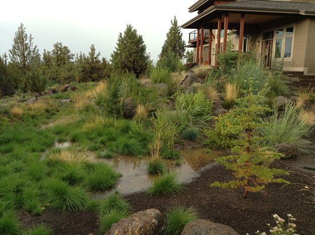
But we don’t always take advantage of that inherent flexibility when we design and manage urban landscapes. Many of us maintain a lawn not because we made a conscious decision that it provides specific benefits we want, but simply because that was what was there when we moved in or because we feel social pressure to conform to the status quo. In Phoenix, Arizona, how people maintain their front yards is partly influenced by what landscape was initially installed when the housing development was constructed. During the region’s housing boom of the 1960s, lawns were the favored landscape installation for new construction, but that has been shifting in recent decades to less water-consuming designs. But many residents of the older developments still maintain legacy lawns even though the lawns don’t match the functions and traits the residents told researchers they wanted their front yards to provide.155
An important approach to improving the resource use efficiency of our urban landscapes is simply to define the services we want a landscape to provide. Setting explicit goals will help us to optimize landscape designs so that we get the most benefit out of them with the minimum cost. The flexibility we have in setting goals and implementing designs can create challenges, however. Just as with farmers, social and economic factors can also shape and constrain urban landscape designs. In 2014, the Metropolitan Water District of Southern California offered cash rebates to entice homeowners into replacing their high-water-use lawns with low-water-use landscapes. The program was popular; before the money ran out, 46,000 rebates were given to replace more than 15.3 million m2 of turf. The popularity of the program suggests that many folks weren’t specifically tied to having a lawn and were more than happy to replace it with some other landscape type if given a reason to—such as a financial incentive. The program did not prescribe what the turf replacement needed to be, just that it needed to meet a low-water-use standard. Homeowners took full advantage of their creative leeway, replacing their turf with everything from a layer of gravel to complex and species-rich native plant landscapes. Most folks who completely replaced their turf front yard did so with non-plant options such as gravel, woodchips, and artificial turf. Many people just let their lawn die and went with a bare soil front yard.156 While saving water, those non-plant options come with the trade-off of reduced ecosystem services such as reduced habitat value and less capacity to mitigate the urban heat island effect. The folks who replaced their lawns with the simplest (and cheapest options) such as bare ground tended to be of lower income than the folks who replaced lawns with low-water-use plants. Did the lawn conversion program inadvertently contribute to greater inequality in the level of ecosystem services between rich and poor areas? We are just beginning to wrestle with these types of questions.
Land Use Efficiency
One of the things people dislike about cities is how crowded they are. But that human density is one of the big advantages cities have in terms of resource use efficiency. For one, many of the resource-consuming activities of our daily lives get more efficient on a per capita basis the closer we live next to each other. Delivering electricity is a great example. Despite Nikola Tesla’s vision of delivering electricity wirelessly,157 it still takes considerable infrastructure in the form of transmission wires, transformers, and switching stations to deliver electricity to end users. It takes proportionally (on a per capita basis) much less of that infrastructure to deliver electricity to thousands of people living within a few square blocks of a large city than it does a couple hundred folks living spread out across isolated rural homesteads. Transportation systems are another good example. While we may dislike the crowded trains and jammed roadways of cities, they are far more efficient at moving people around than a lonely rural road.
Living at high density also saves land, at least in concept. The Burj Khalifa skyscraper in Dubai, United Arab Emirates, manages to convert a ground footprint of about 15,000 m2 into 309,473 m² of living and working space. In principle, the more people we have living close together, the more land we can devote to natural habitat or other uses such as agriculture. In addition, as described above, the sprawling nature of urbanization magnifies its impact beyond the relatively small physical footprint of buildings and asphalt. Policies and planning decisions can foster the development of more compact urban development that limits or mitigates some of the ecological impacts of urban sprawl. Social and economic shifts are spurring private enterprise to develop more land-conserving designs and practices. In aggregate, these policies and practices are referred to using the oxymoronic term of conservation development. An increasingly popular planning tool for limiting urban sprawl is the urban growth boundary. Urban growth boundaries define a perimeter around towns and cities within which urban development is encouraged and beyond which it is discouraged or restricted altogether. In the state of Oregon, every city and metropolitan area is required to define an urban growth boundary.158 Similar planning strategies include creating green belts of open space that encircle cities and strategically creating large, interconnected networks of parks and reserves that mitigate habitat fragmentation.
Anti-sprawl concepts can be applied to smaller spatial scales. For instance, conservation housing developments group individual housing units closely together to form high-density clusters. Instead of each residence having their own individual yard, designers create larger contiguous patches of communal open space (Fig. 8.16). The housing clusters can be arranged to preserve important existing habitat features such as wetlands or forest patches. Even if the open space is managed as a domesticated landscape, the larger and more contiguous patches often provide better habitat value than scattered individual yards. The communal land is also easier to manage in ways that promote resource use efficiency, such as having a single expertly run and managed smart irrigation system. The dense clusters of residences require less impervious surface areas and are more efficient in terms of density-dependent infrastructure such as roads and electrical wiring.159
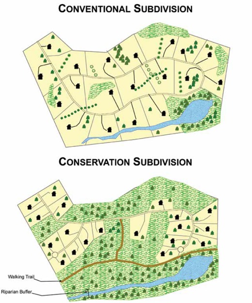
More Efficient Flows
The movement of resources from their source to their eventual urban consumption involves a number of inefficiencies. In Chapter 7 I described a significant one: the roughly one-third to one-half of harvested food that is wasted as it travels up the food supply chain to be eaten. There are similar logistical and supply chain inefficiencies for the range of other resources we consume in cities. The delivery of water to cities is an example. California’s major urban areas are connected to a vast and complex water delivery network that includes the system of reservoirs and aqueducts that store and move water over long distances (see Fig. 3.9), the municipal water systems that distribute water across cities, and the plumbing in individual homes. There are inefficiencies all along the way. A big one is that most of the reservoirs and aqueducts are uncovered, which allows a significant chunk of water to evaporate under the California sunshine before it can reach urban consumers. California’s entire 6,350-km network loses roughly 239,000,000 m3 of water to evaporation each year.160 Leaks are another problem. About 8% of the water in California’s system leaks before it reaches the consumer.161 The systems managed by individual municipal utilities can be even leakier. The US average is a 17% leak loss, with some utilities having a staggering 55% leak loss.162
A potential solution to the evaporation loss is to shade the open-air parts of the network. Solar panels are one idea for providing the shade. One study estimated installing solar panels on California’s system would save 39,000 m3 of water per kilometer of aqueduct per year, in addition to providing clean energy.163 In 2015, the Los Angeles Department of Water and Power took a cheaper approach and covered the surface of the Hollywood Reservoir with more than 96 million opaque plastic balls. The shade balls saved an estimated 1.15 million m3 of water per year. The savings are reduced, however, if we account for the water footprint of the shade balls themselves. Depending on the details of their manufacture, it can take up to 2.9 million m3 of water to manufacture the number of balls used for the Hollywood Reservoir—more than the estimated annual savings in water.164 The city estimates the life span of the balls to be 10 years, so from their perspective, the balls are still a big net benefit in terms of water savings.
The long distances that resources sometimes travel to get to cities also creates inefficiencies. Losses from leaks and evaporation along California’s water delivery system are compounded the farther the water has to travel before it is used. Spatial separation disrupts biologically driven nutrient cycles, and it can be difficult to develop replacement return flows. A prime example of this in urban contexts is what we do with our urine and feces. The nutrients in urine and feces come—via our food—from an often distant farm. We then typically let the nutrients in human waste contaminate a water body, or we bury them in a landfill instead of recycling them to help grow more food. One broad approach to resolving these types of inefficiencies is to develop technologies and strategies that spatially reconnect resource flows or create more circular resource supply chains, to use recycling jargon. An example is sewage treatment technology designed to capture nutrients (principally nitrogen and phosphorus) from municipal wastewater streams and convert them to fertilizer for crops. One study estimated that Europe could meet 20% of its phosphorous needs by capturing and recycling phosphorous from municipal wastewater streams.165 Shortening the spatial separation between resource capture and use could potentially help facilitate the creation of more circular resource flows by exploiting spatially dependent efficiencies, such as locating an urban farm next to a municipal wastewater nutrient recovery system. It would be highly efficient in terms of the transportation and other infrastructure needed to return nutrients to the farm. As you probably suspect, however, approaches such as increasing the use of urban agriculture involve complex trade-offs, constraints, and costs. We are far from understanding what those are, let alone developing optimized strategies. For example, is it better to manage the precious little green space we currently have in urban areas to maximize its value as species habitat (including us) or to maximize its value for food production? While the two goals are not necessarily completely mutually exclusive (see Chap. 7), they still probably involve at least some opposing trade-offs.
8.5 Enriching Social-Ecological Systems
Section 8.5: Enriching Social-Ecological Systems
Urbanization involves a grand trade-off similar to the one we face in our agroecosystems: the more we regulate and control urban conditions, the more we tend to degrade the ability of urban ecosystems to provide functions and services. In proximate terms, as we build hardscape, we degrade the ability of the urban ecosystem to regulate stormwater flows and to capture nutrients, to regulate local temperature, to sequester greenhouse gases, to provide habitat for animals, to improve our quality of life. But the details of that trade-off and how we negotiate it play out in incredibly complex and nuanced ways. That is because people are designing and building the urban landscape, deciding which ecological functions they value, and determining the best way to balance the trade-offs and constraints involved in enhancing their preferred functions. Those human decisions are influenced by economics, cultural identity, social processes, psychology, politics, and the legacy of history. A term that is often used to describe the interaction between human society and ecosystems is a social-ecological system.166 The Anthropocene is a social-ecological system, and much of this book describes social-ecological interactions. Those interactions are particularly evident in urban ecosystems.
We have often designed and built cities in ways that ignored or downplayed their social-ecological interactions, however. Some urban designs have walled us off completely from the natural world. Just is in our agroecosystems, we are beginning to more fully understand the costs of doing that, both in the narrow costs borne by individual city residents and in the broader costs that urbanization accrues for the Earth System. We are also beginning to understand that the trade-off between hardscape and ecological function is not absolute. In many cases, we can design cities that make use of ecological functions and are better integrated with nature. While an urban ecosystem will always be profoundly different than a wildland, new approaches to urban design can significantly enhance the ecosystem functioning of cities. There are several broad approaches.
Green Infrastructure
Green infrastructure is the system of engineered structures that incorporate plants and microbes into their design in order to provide specific ecosystem functions. Most examples of such bio-integrated infrastructure are related to stormwater management (Table 8.2). Sometimes this term is used more broadly to describe all the nonhuman biological assets of a city such as parks, street trees, conservation areas, and rivers. But I like to think of green infrastructure more narrowly as human-engineered structures. These structures are usually designed to meet a specific set of goals and to function under a specific set of constraints.
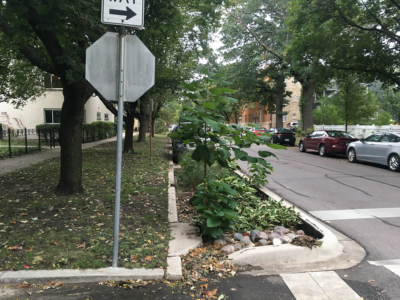
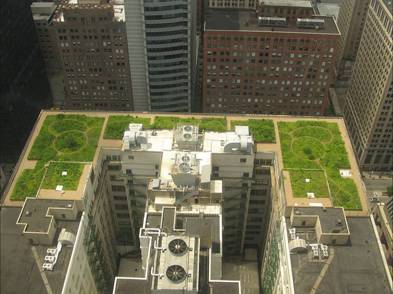
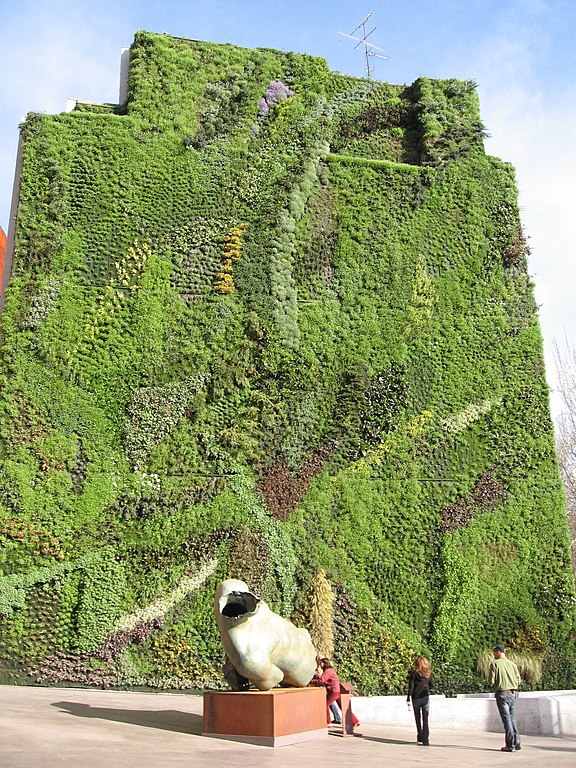
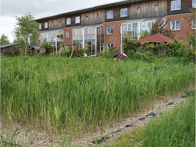
| Examples of Green Infrastructure | ||
|---|---|---|
| Type | Description | Visual Description |
| Bioswales/rain gardens/green streets | Typically relatively small vegetated structures designed to collect surface runoff from hardscape. Goals include increasing stormwater infiltration into the soil and capturing water pollutant |
In downtown Portland, several sewer drains are actually sunken beds of wetland plants that work as phytoremediators, or vegetation that filters toxins. |
| Green Roof | Vegetated roofs consisting of impervious membranes, substrate, and plants. Goals include reducing the volume and slowing the rate of stormwater runoff from roofs, providing building insulation and cooling, and mitigating the urban heat island. |
Often native flora and fauna in raised beds lined by concrete or other less permeable materials; in Chicago’s famous rooftop park, there are many brightly colored rest areas. |
| Green Wall | Plantings installed on interior or exterior walls. Goals include aesthetic and psychological benefits, building insulation and cooling, noise reduction, and mitigating the urban heat island. |
Although typically small, one of the most striking examples is 30 feet tall and woven with bushes, flowers, and ferns–although largely green, there are several striking moments of color. |
| Constructed Wetland | Typically relatively large plantings of wetland species designed to mimic the biophysical traits of natural wetlands. Goals include removing biological, chemical, and thermal pollutants from municipal wastewater or stormwater runoff. | Occasionally seen as unremarkable, Portland, OR has a striking created wetland in Northwest Portland–reeds, tall grasses, and manufactured marsh are bordered by frozen yogurt shops and local sculptures. |
For example, green roofs are primarily designed to reduce the volume and slow the timing of stormwater runoff entering combined sewer systems. Green roofs do this by exploiting the water-regulating functions of soil and plants. A green roof soil absorbs and holds on to rainfall much longer than a normal hardscaped roof. The plants and substrate also evapotranspire a significant amount of the captured rainfall before it can become runoff (Fig. 8.17). In addition to those hydrological functions, green roofs are a structural part of the building, the roof. Therefore many green roofs are designed to be lightweight enough to be installed on buildings without the need for added strengthening or retrofitting. These designs use a thin layer of extremely lightweight soil-like media that is low in organic matter, drains rapidly, and doesn’t retain much water. That keeps the overall weight of the roof (substrate plus stored water) low enough so that it can be installed without special structural modifications to buildings. Green roof plants are chosen for their ability to tolerate the dry conditions created by the quick-draining media as well as the extreme microclimates found on most roofs. This system can be remarkably effective at both attenuating runoff and maintaining healthy vegetation if individual rain events are small in total volume and spaced at moderate (one- to two-week) intervals between periods during which conditions are favorable for photosynthesis. In regions with favorable climates, such as northern Europe and North America, green roofs typically prevent 30% to 60% of the precipitation they intercept from entering municipal stormwater systems.167
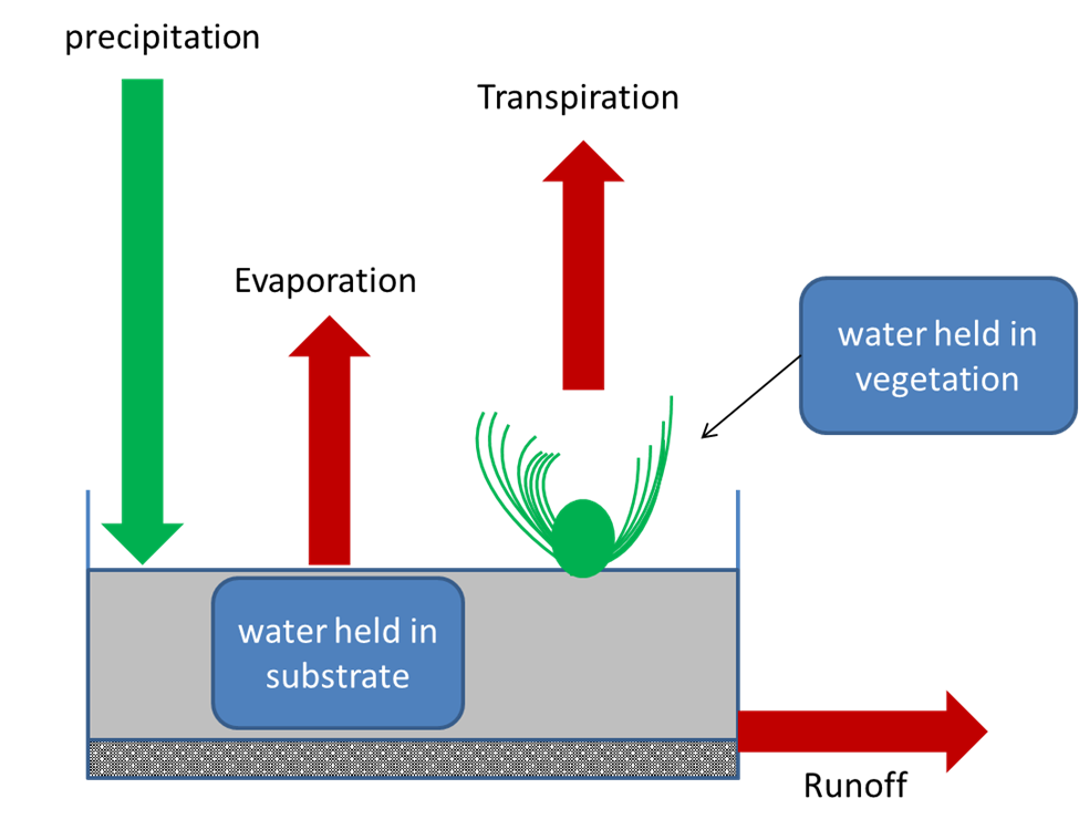
One potential advantage that green infrastructure has over nonbiological infrastructure (often called gray infrastructure) is that it can be cheaper to build or operate. In 2012, Cincinnati, Ohio, had a combined sewer overflow problem that put it in violation of the US Clean Water Act. One proposed solution was to increase the capacity of the stormwater system by constructing a large stormwater tunnel. Instead, the city opted for a plan that involved installing 81 rain gardens on residential properties located across an important watershed of the city. They did this partly because the rain gardens were estimated to be about 42% cheaper to install and maintain than the tunnel. The cost savings were even bigger when they accounted for the environmental costs associated with construction such as greenhouse gas emissions and other pollutants. Rain garden construction was estimated to cause 62% to 98% less environmental impact than building the tunnel would have.168 The fact that much of the direct financial savings of green infrastructure can come early, during the construction phase, is particularly attractive to often cash-strapped cities, and green infrastructure is increasingly being used and promoted both as an alternative to gray infrastructure and as part of integrated systems that combine green and gray elements.169
Green infrastructure has the potential to provide a wider range of functions and services than gray infrastructure. In addition to reducing stormwater runoff, green roofs can help cool and insulate buildings, mitigate the urban heat island, reduce noise pollution, remove air and water pollutants, provide animal habitat, support native biodiversity, and provide beauty and access to nature that translate into human psychological and health benefits.170 In contrast, a stormwater culvert basically provides one service: unobtrusively moving water. We can use the approaches described in Section 2.5 to quantify and value the various services that green infrastructure provide. These valuations are increasingly being used to help inform urban planning decisions. For example, Portland, Oregon, quantified some of the multiple functions and services that its various forms of green infrastructure provide the city (Table 8.3). Based partly on these data, Portland made significant direct investments in green infrastructure. It also promoted the use of green infrastructure by developers, local neighborhoods, and individual residents using financial incentives, educational outreach programs, adjustments to building codes, and regulations. As of 2019, there were almost 400 green roofs alone in the city.171
| Green Infrastructure Benefits in Portland, Oregon | |||
|---|---|---|---|
| Benefit | Green Roofs | Green Streets | Urban Trees |
| Stormwater Flows | 60% peak flow reduction | 93% peak flow reduction | 10% flow reduction |
| Water Pollution | 95% reduction (metals) | 80% reduction (total suspended solids) | No data |
| Air Pollution | 8.6 kg/ha/year removed (PM10) | 0.04 kg/ha/year removed (PM10) | 0.2 kg/tree/year removed (PM10) |
| Greenhouse Gasses | 17.5 t/ha/year removed | 0.7 t/ha/year removed | .3 t/tree/year removed |
| Energy Savings | 20 kWh/ha | 383 kWh/facility | 3 kWh/tree |
| Nature Access | Dependent on roof access and view shed | 2,000 pedestrians/day | 2,000 pedestrians/day |
The trend in recent years has been toward green infrastructure designs that integrate a diverse portfolio of functions. For example, green roof designs can use regionally native plant species chosen for their value as animal habitat with the explicit goal of supporting native biodiversity. The plant choices can match the local environmental conditions and leverage resource complementarity and facilitation so as to minimize the resource inputs required to maintain the roof. The roof can have an aesthetically pleasing design and be made accessible to the public in order to provide beauty and a calming green space for building occupants (Fig. 8.18). Like any biological system, however, the form and function of green infrastructure involve trade-offs and constraints. For example, using shallow, quickly draining substrates on green roofs is a clever approach because, counterintuitively, substrate depth doesn’t have much of an influence on the stormwater mitigation properties of the roof.172 But shallow and organic-matter-poor substrates do constrain the type of plants that can survive on the roof, particularly if the goal is to have a low-resource input system. That restriction on plant functional traits can in turn influence other services, such as the provisioning of wildlife habitat or aesthetics. The diverse community of native plants used on the green roof in Figure 8.18 was partly achieved by using deeper layers of a more natural soil that contains more organic matter.
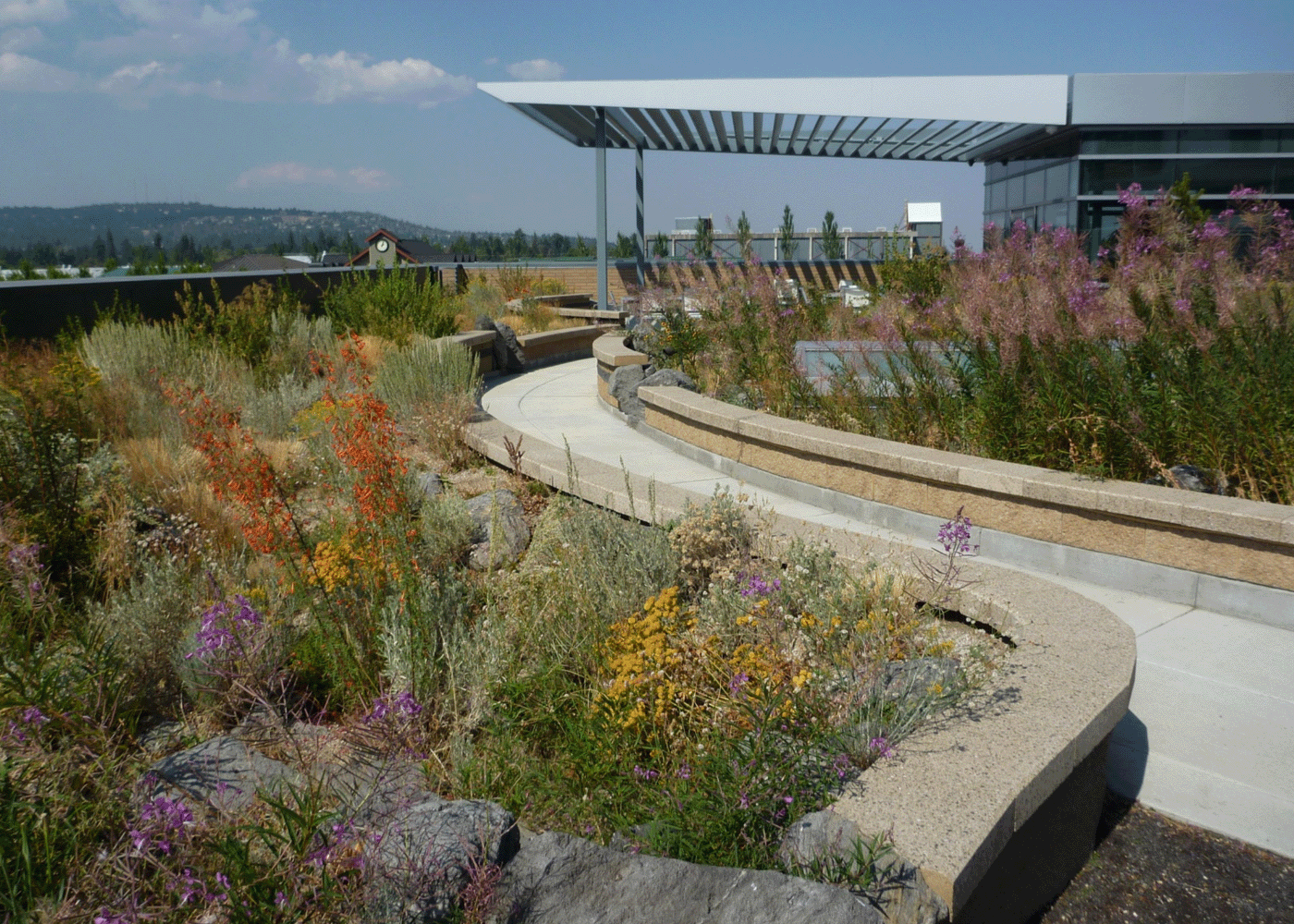
Another set of constraints relates to integrating green infrastructure into the urban landscape. Green infrastructure is often retrofitted into the existing fixed gray infrastructure, or it must work as just one (often ancillary) component of new infrastructure. As a result, green infrastructure tends to be small and isolated. That spatial pattern can limit the ability of green infrastructure to provide some types of functions. Some data suggest that green space needs to be a at least about 0.5 to 2.0 ha in size before it significantly reduces the heat island effect across the scale of a neighborhood,173 so small bits of green infrastructure like a green street might have only a marginal ability to mitigate the urban heat island. But we don’t fully understand how size, shape, and location in the urban landscape influence the various functions of green infrastructure. The degree to which green infrastructure can support biodiversity is a good example. A review of the available data found that green infrastructure such as green roofs and bioswales can support significantly more biodiversity than hardscape. But even when the green infrastructure was specifically designed to function as habitat or otherwise support biodiversity (e.g., by using diverse assemblages of native plants), it did not support any more biodiversity than unplanned habitat fragments such as vacant lots.174 This finding suggests that factors such as the size of the green space and its spatial relationship and connectivity strongly influence how it functions to support biodiversity.
In addition, the degree to which green infrastructure provides direct human benefits such as aesthetic enjoyment, emotional recharge, and improved health is strongly influenced by how the green infrastructure interacts with the social landscape of the city. A number of studies have documented that green roofs can provide a range of psychological benefits, such as providing a calming place to de-stress and to recharge emotionally. The degree to which people experience those benefits depends on a host of social factors, however.175 For example, green roofs are much less accessible than a public park, with access typically limited to building users or maintenance workers. Even when the green roof is open to the public, there can be significant barriers to access. Although a majority of the residents of a public housing complex in Singapore reported regularly visiting ground-level parks, for example, only 18% reported visiting a rooftop garden. The main reasons for the low usage were issues related to accessibility, including not knowing that a roof garden existed or how to access it, and the physical constraint of having to walk up stairs.176
Ecological Intensification of Domesticated Landscapes
We are beginning to design the other parts of our urban domesticated landscapes in ways that enhance their ecological services and functions. Partly this involves just having a better understanding of what those services and functions are. Over most of the time that our cities have been growing, we didn’t appreciate many of the services that our domesticated landscapes provide, such as helping to sequester atmospheric carbon, reducing air pollution, or supporting biodiversity. We also poorly quantified the other things that we did appreciate about them, like beauty, recreation, and shade. Although cities recognized the general importance of their green spaces, they still undervalued them when it came to making land use decisions and investing resources to build and maintain them. Urban forests are a good example. From 2009 to 2014, urban tree cover in the United States dropped by about 1%. That may not sound like much, but it represents a loss of about 36 million trees per year.177 A range of factors have contributed to the loss of tree cover, including the spread of non-native pests and diseases, climate change, and the unavoidable attritional losses due to bad luck and old age. But the net loss reflects the fact that cities have not been investing enough to protect, maintain, and replace their trees. Although hardly anyone dislikes them, trees are often low down on a long list of other priorities and goals.
We are beginning to get more quantitative data about the services urban domesticated landscapes provide. Table 8.3 gives estimates for some of the ecosystem services that street and residential trees provide Portland, Oregon. As with green infrastructure, we can value these services in monetary terms. Just the air pollution removal, carbon sequestration, and reduced building energy not provided by the lost 1% tree cover from 2009 to 2014 is conservatively estimated to have cost US cities $96 million per year.178 And that figure does not account for the value of other services, such as wildlife habitat and the variety of social and psychological benefits associated with tree cover. Impressive valuations like that are beginning to push trees up the priority list of cities, and many have embarked on ambitious tree planting programs.179
Some cities include ecological function as an important consideration when choosing which tree species to plant. For example, as Los Angeles grew, landscape designs evoked a tropical paradise, frequently as a way to sell real estate. Palm trees were favorite elements of the motif (Fig. 8.19). The palms signaled sun, fun, and easy living, particularly for residents of cold northern industrial cities. The fan palm (Washingtonia filifera) in Figure 8.19 was being planted in front of the new Southern Pacific Railroad station. A columnist for the Los Angeles Herald observed that it would give “the Eastern arrival as he proceeds up town a first impression of the wondrous things that are in store for him.”180 There is a good chance that the tree in Figure 8.19 is now the oldest palm tree in Los Angeles, although it was moved from the train station to its present location at the entrance to Exposition Park. Fan palms are native to the deserts of California and Arizona, and once established, they don’t need much in the way of supplemental irrigation in the Mediterranean climate of Los Angeles. That makes them a great landscape choice when water supplies are limited. Divorced from their original ecological context and plunked down in the urban landscape of Los Angeles, however, palms provide a relatively narrow set of ecological functions. As the palms gradually die, the city is now replacing them with species that provide a broader range of services such as more shade to reduce the urban heat island effect.181 The city still plants some palm trees, but now only in strategic tourist attractions such as Hollywood.
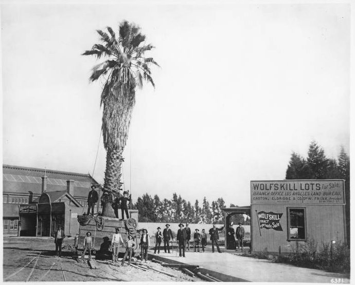
Making the delivery of a broad range of ecological functions an explicit design goal for our urban landscapes is a way to gain the most ecological benefit out of limited urban green space. For example, golf courses often get a bad rap for taking up relatively large swaths of land while providing benefits only golf aficionados appreciate. Just by being significant chunks of green space, however, golf courses (at least urban ones) provide important species habitat as well as other ecosystem services.182 Golf course designers and managers are beginning to better leverage that ecological potential. Techniques include converting roughs into species-diverse meadows, converting water features into more ecologically functional wetlands and riparian zones, removing invasive species and restoring native vegetation in out-of-play areas, minimizing the footprint of intensive management to a few target areas such as putting greens, and using integrative pest management. Similarly, ecologically conscious designs are being developed for the other types of urban domesticated landscapes, such as community gardens, public parks, residential landscapes, cemeteries, and front yards.
Supporting native biodiversity is one function that we are increasingly designing and managing domesticated landscapes to provide. The approaches for enriching the biodiversity of our agroecosystems described in Section 7.5 broadly apply to urban landscapes as well. Also, in Section 8.3, I describe some of the characteristics and management styles that tend to enhance the biodiversity of urban domesticated landscapes. Enhancing urban landscape biodiversity typically involves some combination of the following:
- Planting regionally native species.
- Using functionally diverse plant assemblages that include traits that provide resources or physical habitat for native animal species.
- Designing landscapes that have a high degree of structural complexity.
- Creating diverse physical habitat conditions that support species habitat such as sources of water, bare ground, or unmanaged areas.
- Adjusting the timing or form of physical disturbances such as mowing and pruning so that they better integrate with the life history and phenology of species.
- Eliminating or minimizing the use of chemical pesticides.
The details of how best to implement those approaches vary depending on the region, the climate, the aspect of biodiversity, and the constraints imposed by the local urban context. We are far from understanding all the complexities or figuring out all the details. For instance, we are just starting to accumulate quantitative information on how different garden plants differ in their value to pollinator insects. Ironically, one of the biggest challenges to getting those data is the immense diversity of plant species, varieties, genotypes, and functional forms that we can potentially use in our domesticated landscapes (Fig. 8.20). Collecting pollinator use data for all the potential forms is time consuming and expensive, and to be useful, the studies must be regionally specific. In addition, what we really need to know is how best to combine plant forms and traits so as to maximize their overall combined biodiversity value in a landscape. We are beginning to get those data.
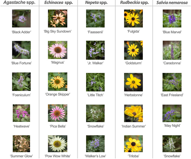
| Description of Floral Cultivars of the Genera Agastache, Echinacea, Redbeckia, Nepeta, and Salvia | |||
|---|---|---|---|
| Genus | Noteworthy Genus Characteristics | Cultivar & Hybridized Species | Botanical Description |
| Agastache spp. Native |
Growth Habit: Clumping; 2-4′ tall. Agastache hybrids often have showier flowers and better winter hardiness than species plants. Inflorescence: Red, Orange, Pink, Yellow, or White; terminal spikes; 2-lipped tubular flowers Vegetative Characters: 2-4′ tall stiff square stems; opposite, serrate, fragrant, gray-green to medium green leaves; fragrance anise/licorice.Hybrids typically feature dense terminal spikes of tiny 2-lipped tubular flowers which bloom mid-summer to fall in many-flowered verticillasters (false whorls) atop 2-4’ tall stiff square stems clad with opposite pairs of serrate, fragrant (anise/licorice scented) gray-green to medium green leaves. Pollinators: Butterflies, Hummingbirds, Bombus spp. |
‘Black Adder’ A. rugosum X A. foeniculum |
Growth Habit: Upright, clump-forming; to 2-3′ tall Distinct Characters: long summer-to-frost floral period; inflorescence smoky red-violet; bottle-brush terminal spikes (6-8″ long). Arrangd in vertillicasters (false whorls); lanceolate to ovate leaves; blue-green. |
| ‘Blue Fortune’ Agastache spp. X ‘Blue Fortune’* |
Growth Habit: Discrete; spreading, 3′ tall; long bloom period, drought tolerant; 2-3′ tall Distinct Characters: Smaller, fuzzier blue blooms; green blue leaves to 4″ long; downy abaxial surface; edible. |
||
| ‘Foeniculum’ A. foeniculum |
Growth Habit: 2-4ft tall; perennial; erect, clumping Distinct Characters: Ovate leaves; toothed; whitish abaxial surface; scent only released when bruised; terminal spikes not in vertillicasters; small blue blooms |
||
| ‘Heatwave’ A. ‘Pink Pop’ varietal |
Growth Habit: 18″ tall; clumping, perennial, erect Distinct Characters: Flowers in whorls on erect, terminal, salvia-like spikes; late spring to early fall blooming; hot pink to hot red. |
||
| ‘Summer Glow’ A. ‘Pink Pop’ X A. ‘Apricot Sunrise’ |
Growth Habit: 1-2; spreading, erect, perennial; spacing 18:-24″; summer bloom period. Distinct Characters: Minty scent; white to custard-yellow tubluar flowers with red stipules; ovate leaves with green abaxial surface. |
||
| Echinacea spp. Native |
A genus of seven species all endemic to Eastern and Central North America. Also known as ‘coneflowers.’ Most cultivars are from purpurea, and characteristics from said species are listed below Growth Habit: Bloom from June to August with some later sporadic blooming; clumping,, multi-stemmed, upright, columnar; self-seeding annual; 2-4′ tall Inflorescence: purpurea is the purple variety; many species only differ by standard floral color; with large blackened cones of disc flowers in center; appears as inverted daisies; terminal, cymous. Vegetative Characteristics: Strigose, toothed dark green leaves, 4-5″; lanceolate Pollinators: goldfinches (however, mostly seed distributive), bees, other insect pollinators |
‘Big Sky Sundown’ Unknown cross U.S. Plant Patent PP17,659 Issued 04/2007 under cultivar ‘Evan Saul’ Can be found as Echinacea ‘Evan Saul’ Big Sky Sundown |
Growth Habit: Clumping; 32-36″ tall; columnar, 18″ wide on sturdy stems, no staking Distinct Characters: Inflorescence lightly fragrant, large, showy, russet-orange ray flowers, dark brown center cones; strigose, coarsely-toothed, dark green lanceolate leaves |
| ‘Magnus’ E. purpurea ‘Magnus’ |
Growth Habit: 2-4′ tall; columnar; self-seeding annual; stems will last well into winter Distinct Characters: broad non-drooping petals; rosy purple; surrounding a brown-black to black cone |
||
| ‘Orange Skipper’ E. ‘Orange You Awesome’ x E. purpurea |
Growth Habit: Named for its ability to attract “skipper” butterflies; well-branched stems; clumping, 1.75′ tall; 1.5′ spread Distinct Characters: Orange-ray florets with red tinted bases; favored by butterflies |
||
| ‘Pica Bella’ E. purpurea ‘Abenstem’ seedling |
Growth Habit: Upright, clumping, 24″-36″ Distinct Characters: Toothed, tapering, narrow-ovate, dark-green leaves; coneflowers more daisy-like, narrow deep pink rays and orange-bronze central bones; bloom June to September. |
||
| ‘Pow Wow White’ E. purpurea ‘Pow Wow White’ |
Growth Habit: Upright, clumping, 2-3′ tall, 1-1.5′ wide; sturdy, branching Distinct Characters: Flowers 3-4″ diameter; downward-arching, overlapping, clean white rays; yellow to yellowish-brown center cone. Late spring to late summer blooming; narrow to ovate leaves; up to 6″ long are medium green. |
||
| Agastache spp. Native Nepeta cataria is the species known as ‘catnip,’ although many are attractive to felines. |
Growth Habit: Spreading, clumping, decumbent ascending and upright stems, although in cataria descended cultivars these are often not very sturdy; 18-2ft tall; spreading as far as 1.5ft-3ft Inflorescence: Small, tubular, pale-lilac to deep violet two-lipped flowers (1/2″ long) clustered in loose raceme-like verticillasters (false whorls) Vegetative Characteristics: Gray-green, hairy, ovate leaves up to 1″ long, crenate margins; prominent veining and heart-shaped bases. Leaves highly aromatic. Pollinators: Cats (rub against flowers; self-pollination), wind, bees. |
‘Faassenii’ Nepeta racemosa X Nepeta nepetella |
Growth Habit: Spreading clump, decumbent, ascending and upright stems; 18-24″; spreading as much as 36″ wide Distinct Characters: gray-green leaves, lavender blue flowers |
| ‘Jr. Walker’ N. ‘Walker’s Low’ X N. xfaassenii |
Growth Habit: 18″-24″; spreads up to 24-36″ Distinct Characters: flowers are quite abundant but less than 1/2″ in petal length |
||
| ‘Little Titch’ N. ‘Walker’s Low’ X N. ‘Jr. Walker’ |
Growth Habit: 18″-24″; spreads up to 24-36″ Distinct Characters: Stems are not as upright as others, leaves less than 1″; flowers less than 1/2″ |
||
| ‘Snowflake’ Nepeta subsellis variant |
Growth Habit: 36″-2ft; clumping, decumbent, ascendant, less than sturdy upright stems; spreading and vining at edges Distinct Characters: Flowers white and showy; leaves with neatly toothed, puckered margins; will weave through rock gardens. Unrecognized by Missouri Botanical Gardens. |
||
| ‘Walker’s Low’ N. racemosa X N. xfaassenii |
Growth Habit: 24-30″ tall–not actually very low Distinct Characters: Loose whorls of small, abundant, two-lipped, trumpet-shaped, lavender-blue flowers. |
||
| Agastache spp. Native |
Growth Habit: Perennial; native to Easter North America; Clump-forming, free-blooming ‘coneflower’ grows to 3′ tall; forms colonies in the wild. Can be invasive and easily get out of hand due to rhizomatous root structure. Inflorescence: Daisy-like, 2.5″ across flowers; yellow rays and brownish-purple center disks. Prolific bloomer. Vegetative Characteristics: Oblong to lanceolate, medium-green foliage. Pollinators: Butterflies, insect pollinators (some bees, but mostly alternative insects); Birds eat seeds. |
‘Fulgida’ R. fulgida** |
Growth Habit: Considered the ‘base form’ for most cultivars. Distinct Characters: No particularly unique characters. Many cultivars descend from R. fulgida |
| ‘Goldsturm’ R. fulgida var. sullivantii ‘Goldsturm’** |
Growth Habit: Native to swamps; shorelines; fens; sedge meadows; upright; rhizomatous; clump-forming perennial 2-3′ tall. Distinct Characters: Flowers daisy-like, 3-4″ across, deep yellow rays and dark brown-black to black disks. Flowers in cymes (singular) on stiff, branching stems; mid-summer to fall. Oblong to lanceolate leaves. |
||
| ‘Herbstonne’ R. nitida X R. laciniata |
Growth Habit: Upright, rhizomatous, clump-forming perennial ‘coneflower’; 4-7′ tall Distinct Characters: Flowers 3-4″ across; daisy-like; drooping yellow rays and elongated, bright green center cones. Cymous, slender branching stems; late summer bloomer. Toothed, bright green, lanceolate leaves. |
||
| ‘Indian Summer’ R. hirta ‘Indian Summer’*** |
Growth Habit: Biennial, 2-3′ tall; rhizomatous, stiff, leafy stems, rarely branched; sometimes weedy Distinct Characters: Huge flowerheads, 6-9″ in diameter compared to R. hirta proper; come in shades of red, yellow, bronze, orange, and bicolors; sometimes called ‘gloriosa daisy |
||
| ‘Triloba’**** R. triloba |
Growth Habit: Coarse, weedy, somewhat hairy, clump-forming; densely-branched biennial or short-lived perennial that is native more to the Midwest than other Rudbeckia Distinct Characters: Flowers are 1-1 1/2″ across; daisy-like; distinguished from R. hirta by smaller, more profuse blooming; fewer rays per flowerhead; leaves are lobed, often 3, less frequently 5-7; lower leaves are ovate to ovate-cordate with long petioles, upper leaves less rounded, sessile (attached at the stem). |
||
| Agastache spp. Native |
Growth Habit: Erect, many-branched, woody-based, clumping perennial; 1.5-3′ tall; 2′ wide. Inflorescence: Lavender to violet blue flowers; .5″ long; subtended by reddish-purple bracts; June to September blooming. Terminal, upright, spike-like racemes that rise well above the foliage. Vegetative Characteristics: Leaves are mostly on lower third of the plant; notched, wrinkled, ovate-lanceolate to oblong, medium green to gray-green, up to 4″; aromatic when bruised. Pollinators: Bees (Bombus, Osmia, Apis), Butterflies |
‘Blue Marvel’ S. nemarosa ‘Blue Marvel’ |
Growth Habit: 9″-12″ tall; 1-1 1/2 ft wide; upright, inflorescence well above foliage Distinct Characters: reportedly will bloom darkest and brightest of any salvia, also referred to as ‘New Dimension Blue’; bloom the first year; May to August bloom period. |
| ‘Caradonna’ S. nemarosa ‘Caradonna’ |
Growth Habit: erect, clump-forming, perennial Distinct Characters: Dark-purple stems; blue-violet flowers. Foliage mound roughly 12″ tall. Inflorescence dense terminal spikes rise to 24″ tall. |
||
| ‘East Friesland’ S. nemarosa ‘East Friesland’ (‘Ostfriesland’) |
Growth Habit: foliage to 10″ tall; erect, clump-forming perennial Distinct Characters: Wrinkled, lance-shaped, light green leaves (up to 4″ long); inflorescence up to 18″ tall; dense-terminal violet-purple |
||
| ‘May Night’ S. nemarosa X S. sylvestris ‘May Night’ (‘mainacht’) |
Growth Habit: Branched, upright, 12-18″ tall; 18-24″ wide Distinct Characters: Dark violet-blue flower spikes; foliage is blue-green. Related to Salvia x sylvestris ‘Little Night’ |
||
| ‘Snowflake’ S. nemarosa ‘Snowflake’ S. nemarosa ‘Eveline’ |
Growth Habit: Upright, clump-forming, compact; dense basal branching habit Distinct Characters: Two-toned pink and purple flowers from mid-spring to early summer, mixed with white flowers that bloom occasionally longer; sage-like fragrance; flowering stems can rise to 20″ |
||
| Notes | |||
| *: ‘Blue Fortune’ is a European hybrid, but Agastache the genus is native to the Americas. | |||
| **: Rudbeckia fulgida and R. fulgida var. sullivantii rarely sold by nurseries as cultivars of R. fulgida are quite magnificent; ‘Goldsturm’ is much more valued than var. sullivantii, for example. | |||
| ***: Rudbeckia hirta is also known as black-eyed Susan; hirta means ‘hairy.’ | |||
| ****: Other names for Rudbeckia triloba include brown-eyed Susan,, thin-leaved coneflower, and three-lobed coneflower | |||
Genus name comes from the Greek words agan meaning “very much” and stachys meaning “ear of wheat” in reference to the appearance of the flower spikes.
Researchers planted garden plots in northeastern Pennsylvania using the herbaceous perennial cultivars in Figure 8.20. They found that, overall, the herbaceous perennials supported an abundant and diverse group of arthropod pollinators—mostly bees. But there was considerable variation in the pollinator visitation rates across the 25 plant taxa. In addition, the plant taxa differed in what species of pollinator they attracted. We can use that information to intensify the pollinator support functions of garden designs. A garden plan that used the six most attractive cultivars would attract nearly four times as many bee species than one that used the six least attractive cultivars. The pollinator-intensive planting would also attract several rare and specialist species. The plant taxa also differ in their flowering phenology, and thus the seasonal timing of when they are most attractive to pollinators (Fig. 8.21). We can use that information to design gardens that provide a consistent supply of floral resources to pollinators.
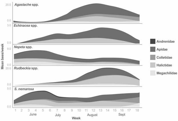
Gaining a better understanding of how best to ecologically intensify urban landscapes is only part of the solution. We also need to implement the ecological designs and management approaches. That can be challenging, given that urban landscape managers have varying levels of knowledge and experience, are variously engaged in the management of their landscapes, have different financial capacity, prioritize functions differently, and have various aesthetic preferences. All those differences can create considerable variation in the types and amount of ecosystem functions urban landscapes provide. For example, residential gardens in Bristol, United Kingdom, differ markedly in the amount of nectar they provide pollinators, with some gardens producing 700 times more pollinator available sugar than other gardens. Those differences primarily reflect differences in the plants making up the gardens, not more immutable constraints such as the size of the garden.183 There is some evidence that people are open to designing and managing more pollinator-friendly gardens, but they need guidance on how to do so. A survey of nonprofessional gardeners in Germany found that although they strongly supported bee-friendly gardening, they did poorly at differentiating the relative pollinator suitability of plant choices.184 Some ways to facilitate design changes include providing practical information such as pollinator-friendly garden designs that are regionally appropriate and straightforward to implement.185 as well as developing outreach efforts like the Million Pollinator Garden Challenge, which established a network of more than million pollinator gardens across the United States (Fig. 8.22).
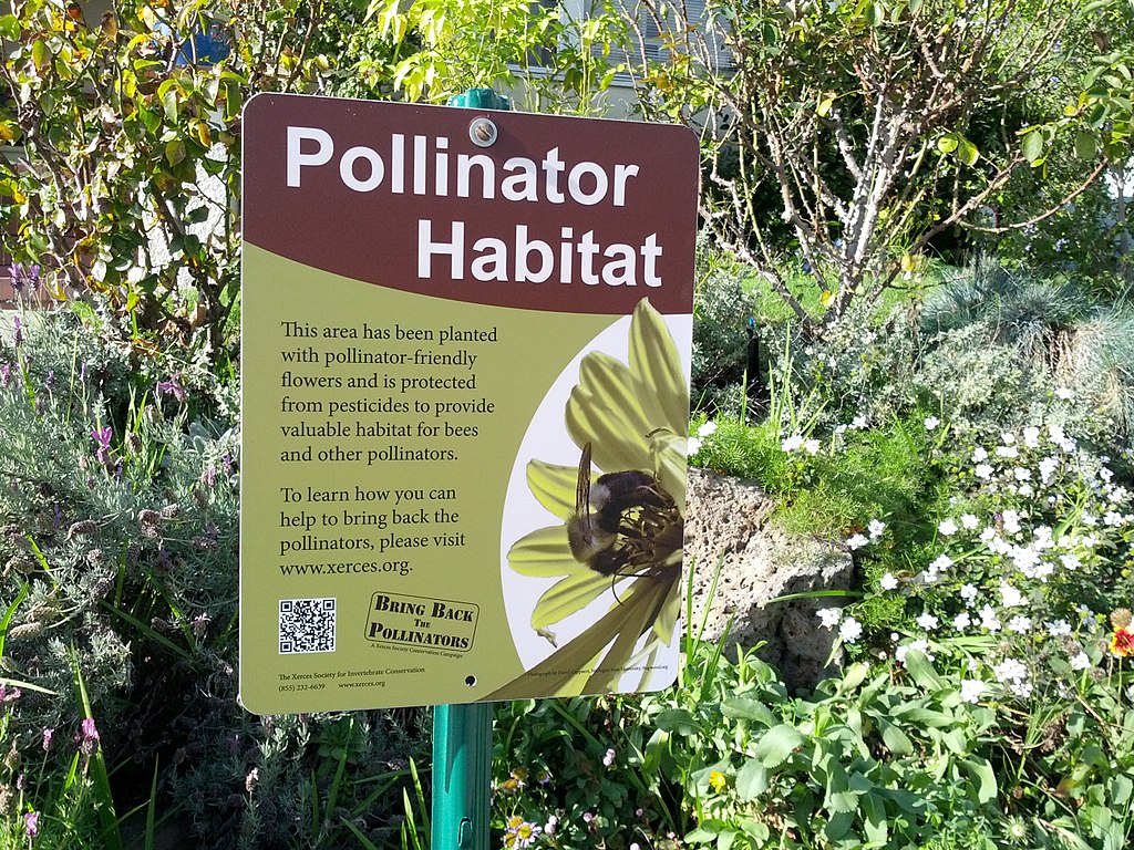
Another complication that we haven’t yet figured out is how best to optimize the portfolio of services that green landscapes generate. At one level, this involves balancing the trade-offs associated with the functional traits of organisms. For instance, a native cultivar might provide suitable resources for native generalist pollinators but have little value for native herbivores. Management actions can also affect the different components of biodiversity in opposite ways, such as how mulching is good for soil-dwelling organisms but reduces habitat for ground-nesting bees (Section 8.3). But perhaps the most important and difficult-to-negotiate trade-offs involve the different goals we have for our urban landscapes. We all have varying cultural backgrounds, family histories, life circumstances, needs, desires, expectations, capacities, tastes—all of which are reflected in the functions we want our urban landscapes to perform. That can create trade-offs—and potential conflict. A quantitative description of such potential trade-offs comes from a study that asked people in the United Kingdom what ecosystem services they wanted from brownfield sites. Brownfields are plots of land occupied by currently unused gray infrastructure such as former industrial sites. The study’s authors asked real estate developers, business owners, workers, city managers, planners and architects, and the public to list all the potential ecosystem services the brownfield sites could be designed to provide, and what their relative preferences for the services were. Survey respondents fell into two distinct groups that had two very different visions (Fig. 8.23). One group had a strong preference for services related to biodiversity conservation and education, while another group preferred services related to development, food production, and recreation.
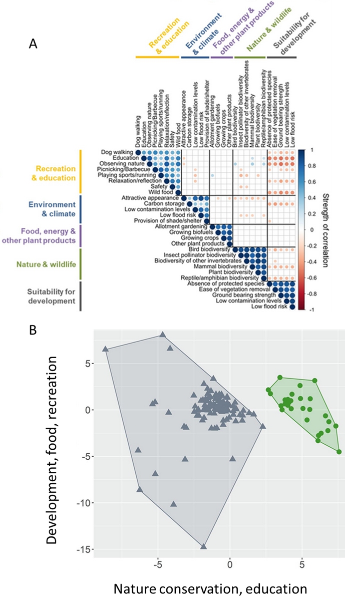
On one hand, the results reflect the seemingly intractably polarized trade-off between real estate developers and conservationists, but there is a more subtle aspect of that polarization. Some people wanted the brownfields to emphasize functions related to community livability such as affordable housing, places to play sports and walk the dog, and community gardens. Others wanted the spaces to emphasize the preservation of nature and to provide refuges where urban residents could experience nature. On the other hand, the survey results found common ground in the fact that people generally wanted the brown sites to provide a wide range of functions. As I have illustrated, many of the disparate goals are potentially compatible—a community garden can be designed to support a diversity of pollinators, while a residential development can be designed to conserve a chunk of wildlife habitat. Figuring out how to best integrate these functions in ways that are relevant to and supported by local communities is one of our big challenges.186
Create Ecological Corridors and Edges
Many of the negative ecological effects associated with urbanization are related to its sprawling spatial pattern (Section 8.1). These negative effects are generated in two interrelated ways. One way is habitat fragmentation. Sprawl fragments contiguous nonurban habitat into smaller isolated fragments. That process can be just as detrimental to the long-term sustainability of populations as is the direct loss of habitat itself. Small bits of habitat often don’t provide enough resources by themselves to support viable populations. They also have proportionally much more wildland-urban interface than do large chunks, which can further degrade their overall habitat quality. Even if a fragment is large enough to support a population, the isolation created by barriers can severely reduce dispersal and genetic interchange, leading to inbreeding, while the barriers themselves (e.g., roads) can kill organisms. The other way sprawl causes problems is by altering ecological flows between the urban and nonurban parts of landscapes. Hardscape can facilitate the flow of urban conditions and materials into nonurban areas, causing negative consequences for the recipients. Light, sound, heat, and nutrient pollution are good examples. Hardscape can also block the flow of nonurban conditions and materials into urban areas. We often do this intentionally, such as when we build levees and walls to protect urban areas from flooding. But these blockages may reduce the provisioning of ecosystem services to urban areas, such as groundwater recharge, water purification, and our own access to the psychological and recreational benefits provided by nature. Newer approaches attempt to mitigate the negative consequences of urban sprawl that focus both on the fragmentation and on the ecological flows.
Reduce Habitat Fragmentation
I already mentioned some of the general approaches to reducing the habitat fragmentation associated with urbanization in the section on land use efficiency. These include increasing human urban density, employing sprawl inhibiting zoning and other land use restrictions, and using more conservation-oriented practices when building new residential development. We can couple those strategies with better information about the space and habitat requirements of organisms. One tool for doing that is called population viability analysis (PVA). PVA combines data on organism ecology with spatially explicit demographic models to evaluate whether an existing landscape can sustainably support species populations. PVA is what researchers used to sound the alarm that Southern California populations of mountain lions are in trouble (Section 8.1). PVA can also be used as a planning tool to design optimal networks of habitat that reduce ecotone effects and that ensure dispersal connectivity. PVA can identify particularly important patches of habitat that should be priorities for conservation. It can also identify the important dispersal and migration corridors that should be the focus of mitigation efforts. Researchers used PVA to understand how urbanization along the expanding edge of Perth, Australia, was likely to affect populations of the southern brown bandicoot (Isoodon obesulus). The overall conclusion was not good. While the diminutive bandicoots can persist in small habitat fragments, the isolation created by roads and buildings causes genetic and demographic decline and ultimately a high risk of local extinction.187 But the researchers predict that the worst declines can be avoided by taking proactive conservation efforts, including preserving and enhancing the existing habitat and creating dispersal corridors that link the habitat patches into a connected network.
One tool for creating dispersal corridors is a wildlife crossing. Wildlife crossings are typically bridges or tunnels that provide a relatively safe passageway over or under a barrier such as a road. Crossings can be incidental structures such as culverts that wildlife use opportunistically. Because these structures weren’t specifically designed as wildlife passageways, they often have access issues, but retrofits such as installing ramps can make them more accessible (Fig. 8.24).
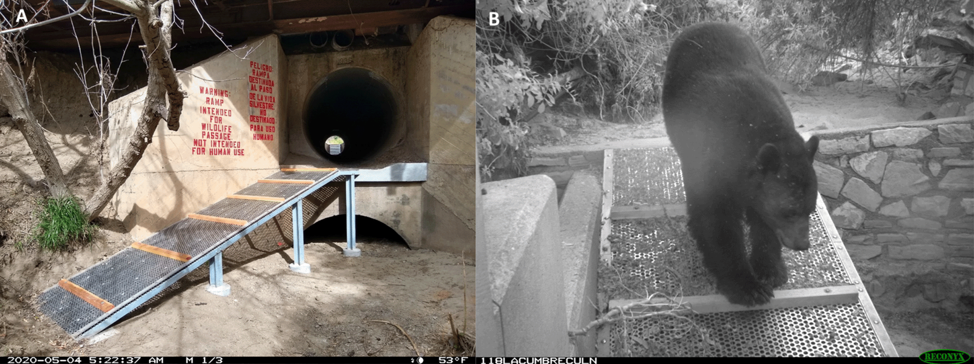
We can also design purpose-built wildlife crossings, as depicted in Figure 8.25. Purpose-built structures can be optimally placed at critical points where wildlife are known to cross or where PVA indicates improved dispersal between isolated populations would have the most benefit. What will be the world’s largest wildlife crossing is being constructed across US Highway 101 in Agoura Hills, California. The crossing is located near the label for mountain lion P-23 in Figure 8.4. That stretch of freeway (plus an adjacent access road) is 10 lanes wide and carries 300,000 vehicles per day.188 The location was chosen because it will connect two significant chunks of habitat: the Santa Monica Mountains to the south and the Simi Hills and Santa Susana Mountains to the north. We also know from roadkill statistics as well as the few radio-tracked animals that manage to cross successfully that animals often try to cross the freeway at that spot. Fencing that stretches along both sides of the freeway will help funnel animals to the crossing. Data from already-constructed crossings indicate that a wide variety of animals use crossings, and sometimes at a high frequency.189 But we still don’t have a good understanding of how animals interact with the crossings. In some cases, passage use seems to involve some degree of cultural learning. In Banff National Park, Canada, some species took up to five years before they were comfortable using the crossings, suggesting they learned how to use the crossings and that information was shared among individuals.190 We don’t have a good understanding of the degree to which crossings improve the long-term viability of populations.
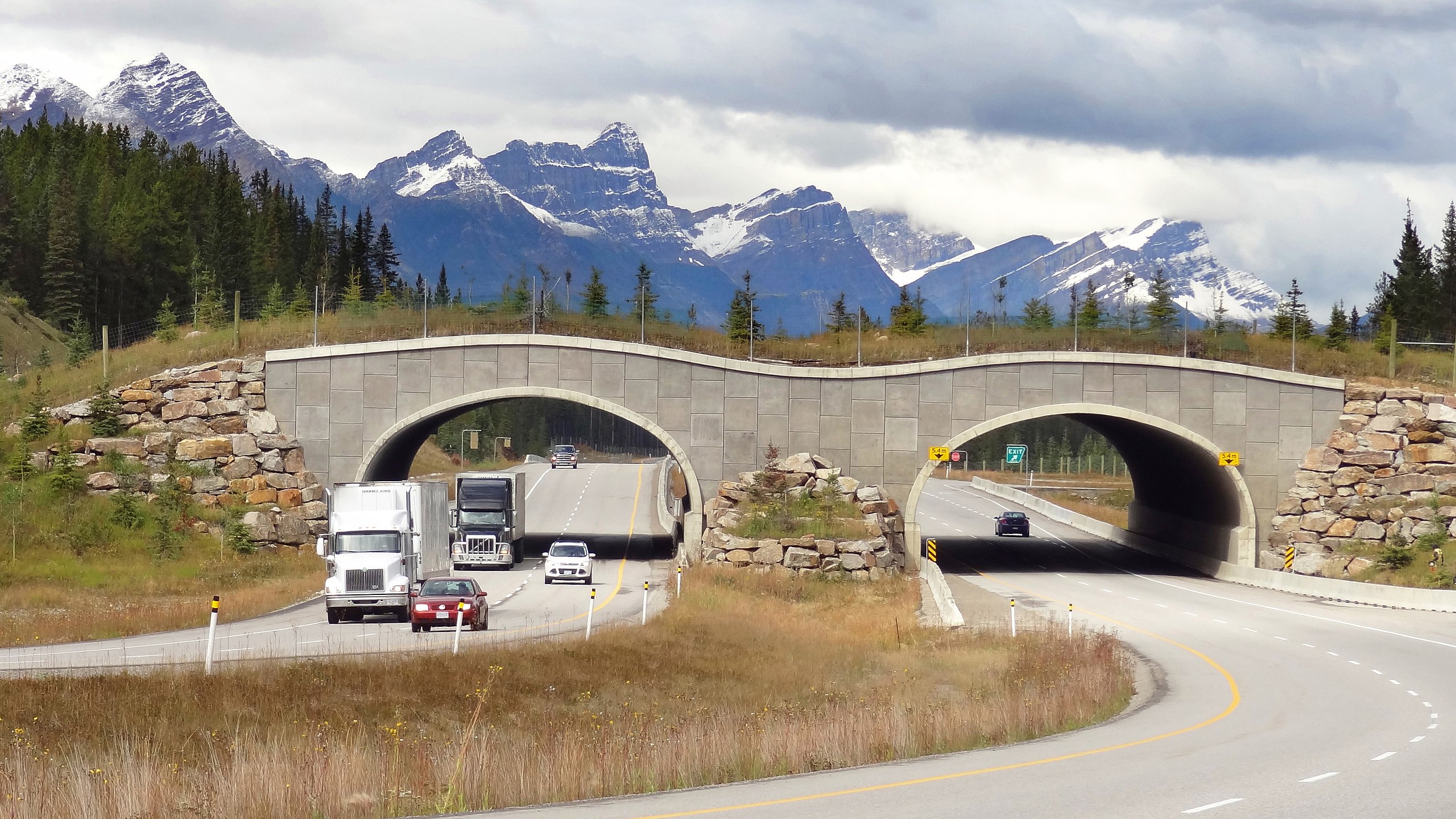
Create More Ecological Urban Edges
Many of the ecological flows from urban to nonurban landscapes occur almost as accidents of our urban activities and designs. We can mitigate many of these accidental flows with more mindful designs. Examples include redesigning streetlamps to reduce the spread of light pollution, using green infrastructure to reduce chemical pollutants flowing into water bodies, and implementing education programs to reduce the availability of human-generated food sources that attract wildlife along the wildland-urban interface.
In contrast, we often try to tightly regulate the ecological flows coming into urban landscapes from nonurban ones. We are beginning to better understand the trade-offs and consequences related to how we regulate those incoming flows. A salient example is our management of flowing water.
We have a conflicted relationship with aquatic ecosystems. We have built the majority of our cities adjacent to them, attracted by their rich ecosystem services such as food, fresh water, and transportation. But aquatic ecosystems are intrinsically dynamic: tides ebb and flow, water levels fluctuate, rivers meander. Indeed, much of the rich biodiversity and ecological productivity of aquatic ecosystems is related to their dynamic flows. That dynamism conflicts with the fixed and rigid nature of our urban hardscape, however. When we build a bridge, we don’t want an overflowing river to quickly destroy it. We don’t want the beach under a coastal house to erode, a shipping channel to silt up, or a low-lying neighborhood to flood. Over much of the nineteenth and twentieth centuries, the general approach to solving those types of conflicts was to reduce the dynamic nature of aquatic ecosystems with even more hardscape. But walling off cites from aquatic ecosystems also walls them off from the ecosystem services aquatic ecosystems provide.
A good example of this approach and its consequences is how Los Angeles developed in relationship to its river. The Tongva people first established a settlement along the Los Angeles River at what would later become downtown.191 Subsequent European colonists also found the riverside location appealing. But by the late 1920s, the city of Los Angeles—sort of like an adolescent chaffing against its parents—was having issues with its river. The fixed infrastructure of the growing city was increasingly at risk from the periodic floods and meandering channels that were an inherent part of the river’s nature. The solution was to turn the river and its tributaries into a mostly concrete channel regulated by a series of dams, with one primary purpose: to move water out of the city as quickly as possible. Figure 8.26 illustrates how this process played out at one stretch of the Arroyo Seco, a tributary of the Los Angeles River (see also Fig. 3.14F for a picture of the main Los Angeles River channel today).
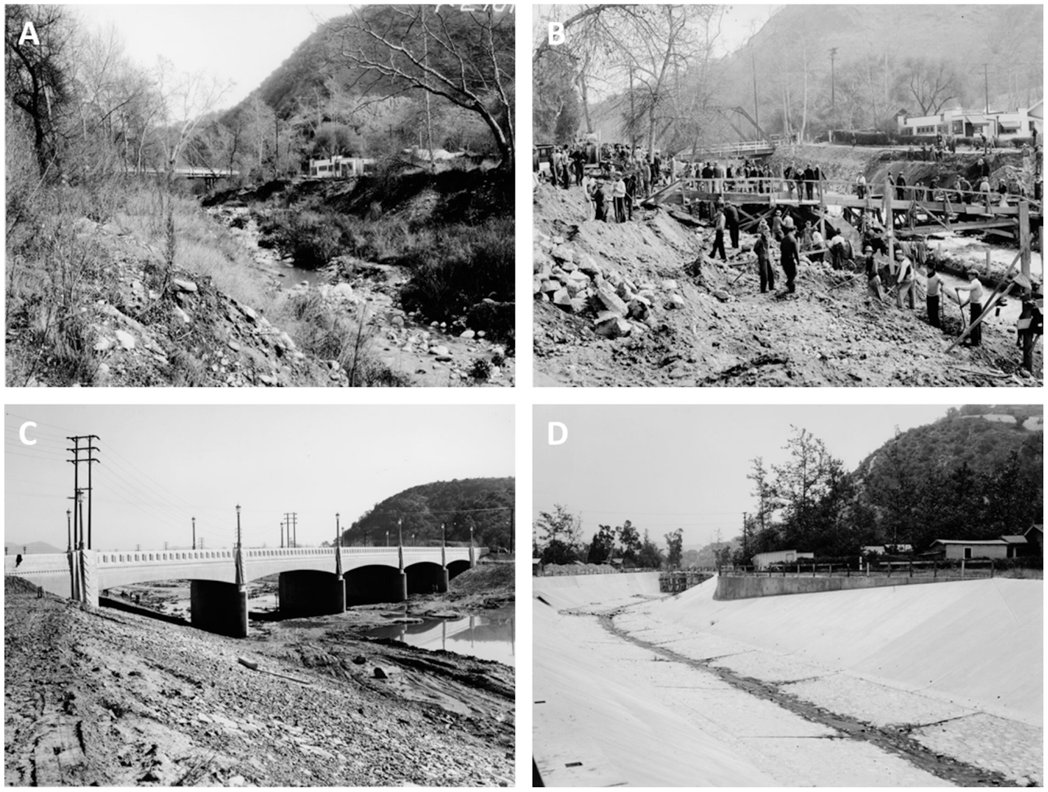
There were other possible paths. In 1930, the Olmsted Brothers landscape architecture firm (successor to the company founded by the famed landscape architect Frederick Law Olmsted) offered the city a different solution to its growing conflict with its rivers. They said the city should move much of the static infrastructure like homes and businesses out of the risky floodplain and mostly let the river do what it wanted to do. Instead of being filled with gray infrastructure, the river’s course and adjacent floodplain could be converted into a network of public parks. The parks would provide immense social value to city residents, while at the same time being much more resilient to periodic flooding than homes, factories, and offices. In retrospect, we now recognize the range of other benefits that preserving the natural river dynamics would have provided such as species habitat, carbon sequestration, urban heat island amelioration, and reductions to air and water pollution. Perhaps most annoyingly, during every rainstorm, residents of the increasingly water-stressed city watch as fresh water is efficiently removed from the city and dumped into the Pacific Ocean instead of recharging groundwater supplies. In fact, during a big rainstorm, more water is moved to the ocean than the city uses in a year.192 The city largely ignored the Olmstead advice and went about adjusting the river to fit into the fixed urban environment instead of adjusting the growing city to accommodate the dynamic nature of the river.
But we are beginning to redesign the border between urban and aquatic ecosystems in ways that restore ecological processes. Los Angeles has started an ambitious project to restore sections of its river system in ways that resemble the Olmsted plan. At strategic points—such as the confluence of the Aroyo Seco and the main channel of the Los Angeles River—the city hopes to move back flood walls, remove concrete, plant native vegetation, and restore public access to the river (Fig. 8.27).
Los Angeles is not alone. Cities around the world are trying a variety of approaches that share the common goal of reintegrating the rigid hardscape of cities with the natural dynamics of their aquatic ecosystems. These include daylighting streams and rivers that had been buried under hardscape; burying gray infrastructure such as roads to restore public access to shorelines and riverbanks; imposing strict building restrictions in coastal zones and floodplains; removing gray infrastructure such as dams, jetties, levees, and sea walls that impede natural flows of water and sediment; using green infrastructure to ecologically buffer the transition between hardscape and aquatic ecosystems; and restoring natural habitat such as wetlands and dune systems along urban margins.
Many of these projects are amalgams of green infrastructure, domesticated landscapes, and remnant natural vegetation. They also balance the trade-offs among ecological services they are designed to provide depending on local contexts and constraints. In some cases, it is possible to restore natural processes and dynamics even within an otherwise highly urbanized area. One example is the restoration of tidal saltmarsh and sand dunes at Crissy Field in San Francisco, California (Fig. 8.28). As you can tell from the pictures, the site is still constrained by urban hardscape, but because the site was a decommissioned military base, planners had more leeway to remove hardscape and reconnect the site to San Francisco Bay than they would have in almost any other part of the city. That made it possible to make restoring the ecological functions and processes of a saltmarsh explicit goals of the project.
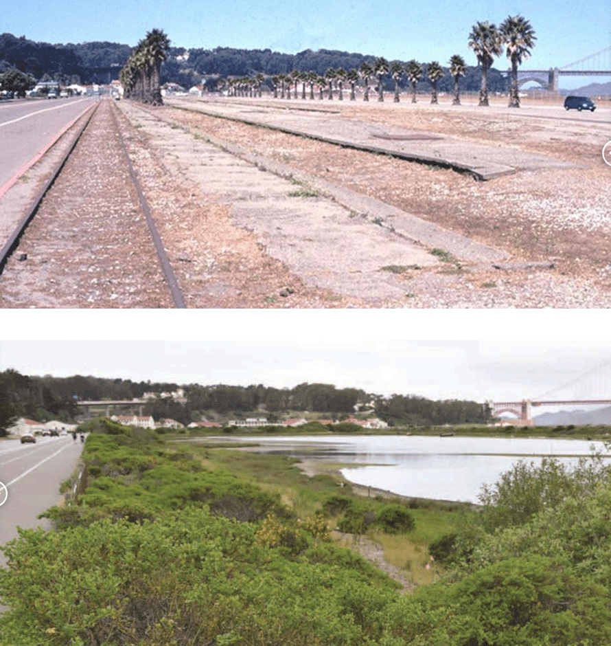
Surprisingly, some of the leading promoters of reestablishing natural flows of water in urban spaces are the Dutch, who are famous for their ability subdue the forces of aquatic ecosystems using hardscape. Twenty-six percent of the Netherlands (where the majority of its population lives) sits below sea level, protected by a complex network of dykes, levees, canals, storm barriers, and pumping stations.”193 But the Dutch are worried that climate change will compromise the long-term sustainability of their system. Increases in sea level and in the severity and frequency of storms are predicted to create conditions that will increasingly exceed the design capacity of the existing system. So, the Dutch are implementing a comprehensive plan to make the system more robust. The plan involves some old standby approaches, such as raising the height of levees. But much of the plan reflects a fundamental shift in design philosophy that aims to work with aquatic systems instead of trying to wall them off. An example of this is the Room for the River Program, a massive public works project that is redesigning stretches of rivers at more than 30 locations across the Netherlands. The details of each project differ, but basically the plans involve moving river levees back to something approximating the more natural floodplain. This will increase the water storage capacity of the rivers, thus keeping water out of heavily urbanized areas. Planners also considered the broader set of ecosystem services that restoring more natural river flows provides, such as improved habitat for aquatic species. In many of the specific projects, homes and businesses are being removed from the now-wider floodplain and being replaced with parks and restored conservation areas—just like what the Olmsted Brothers firm wanted to do with the Los Angeles River.
Improve Ecological Equity
As described above, the provisioning of ecosystem services is not equitably distributed across cities. The disparities stem from the range of social and economic factors that contribute to disparities and injustices in the other aspects of people’s lives. Those often include systemic racism as well as structural barriers that intensify inequities rather than ameliorate them. As we enhance the overall ecosystem services that urban areas generate, we also need to find ways to ensure that urban residents benefit equitably from them.
One first step in doing that is simply to better understand how ecosystem services vary across the spatial, social, racial, and economic geography of a city. We can use that information to identify areas that are impoverished in terms of ecosystem services, as well as areas where improving ecosystem services will have the most impact in people’s lives. For example, the degree to which adding green space results in a reduction of the urban heat island is not uniform across the landscape of a city. The cooling impact of adding trees or other green space is much greater in areas dominated by hardscape than in areas that already have a lot of green space.194 But the degree of cooling is only one aspect of impact. As described in Section 8.3, poor and minority communities tend to have significantly less green space than richer and whiter communities. In addition, poor people have few resources and little capacity to mitigate the problems associated with the lack of ecosystem services. Mitigating capacities are things such as health insurance to cover the cost of an asthma-related emergency room visit, or cash to get the air conditioner fixed, or a car to drive to a distant park to de-stress. That makes the value of ecosystem services far greater in poor areas than in rich ones. While more green space might shave a few dollars off electricity bills in a wealthy neighborhood, it might save several lives in a poor one.
We can use that type of information to prioritize where to create and enhance urban green space. For instance, tree-planting programs can focus on parts of the city where the trees will improve the lives of people the most, such as neighborhoods that suffer particularly acute air pollution or where many of the residents don’t have air conditioning.195 Doing this is not as straightforward as it may at first seem, however. One issue is that programs and policies aimed at enhancing green space are often not implemented in ways that address inequities. For example, Million Trees NYC was a public-private partnership that successfully planted a million trees in the city. But the initiative largely failed to meet its stated goal of correcting inequities in tree abundance. Most of the trees ended up being planted in existing parks, and those parks were more likely to be in wealthier, whiter parts of the city that already had relatively high tree cover. Trees were planted in poorer areas and in communities of color, but not to a degree that alleviated the existing inequality in tree cover. Although environmental justice was a vague goal of the project, it wasn’t reflected in the practical details of how the project was implemented.196
Attempts to ecologically intensify cities are also often refracted through lenses of history, power, privilege, and inequality. In the aftermath of Hurricane Katrina, initial recovery plans envisioned a city with a smaller hardscaped footprint. The smaller footprint would save the city money and resources in rebuilding infrastructure. It would also concentrate rebuilding efforts in areas that had a large enough nucleus of returning people to develop strong social support networks. The reduced hardscape would free up space for more green space that would deliver a range of ecosystem services that the city was lacking, such as food production, recreational open space, and storm-water management. It would also remove some of the people and infrastructure from the areas at highest risk of flood. In 2006, the Times-Picayune published a composite stylized rendition of early planning maps that had large green dots over neighborhoods that were proposed to be downsized. Several of the green dots sat on neighborhoods such as the Lower Ninth Ward that were significant parts New Orleans’s Black heritage, and nearly all the dots were in predominately Black middle- or low-income parts of the city. That pattern reflected centuries of racism and inequality that had forced Black residents to live in parts of the city with the highest flood risk—and that were the worst affected by Hurricane Katrina and the failure of the levee system. It also reflected more current inequities that differentially hindered poorer, largely Black residents from returning to the city relative to wealthier, largely white residents. For many, the green dot map, as it came to be known, was a map of racist disenfranchisement, not a map of ecologically intensified rebirth.197
The political furor that ensued squashed the downsizing approach. In some of the green dot neighborhoods such as Broadmoor, communities mobilized to lead recovery efforts on their own terms. But the governmental recovery response largely failed the poorest and most vulnerable displaced people. Some of the poorest and hardest-hit neighborhoods such as the Lower Ninth Ward are still an echo of their pre-storm condition.198
The recovery of the city’s green space has also been influenced by the racial and economic geography in more individual ways. The inability or unwillingness of some displaced residents to return and rebuild created de facto new green space in the form of abandoned lots, mostly in the poorest and hardest hit parts of the city. How these abandoned lots are managed varies widely. Some lots are managed as turf grass lawns. Some have been converted into community gardens. Others are unmanaged and have developed complex ruderal vegetation (Fig. 8.29). Each of these landscape types provides a different suite of ecosystem services as well as trade-offs and constraints. The lawns provide little in the way of biodiversity, but they help to maintain the property values of adjacent homes. The gardens potentially improve the food security of the neighborhood, but the neighborhoods they are in often have little social cohesion (the strength of relationships and connectedness among community members) that would enhance the garden’s impact. The unmanaged lots can provide habitat for beneficial species such as pollinators, sequester high rates of carbon, and provide storm-water management. But they can also support invasive non-native species, harbor human pests such as rats, and attract illegal activity such as trash dumping.199 Determining how to balance those services, disservices, and constraints is a difficult task.
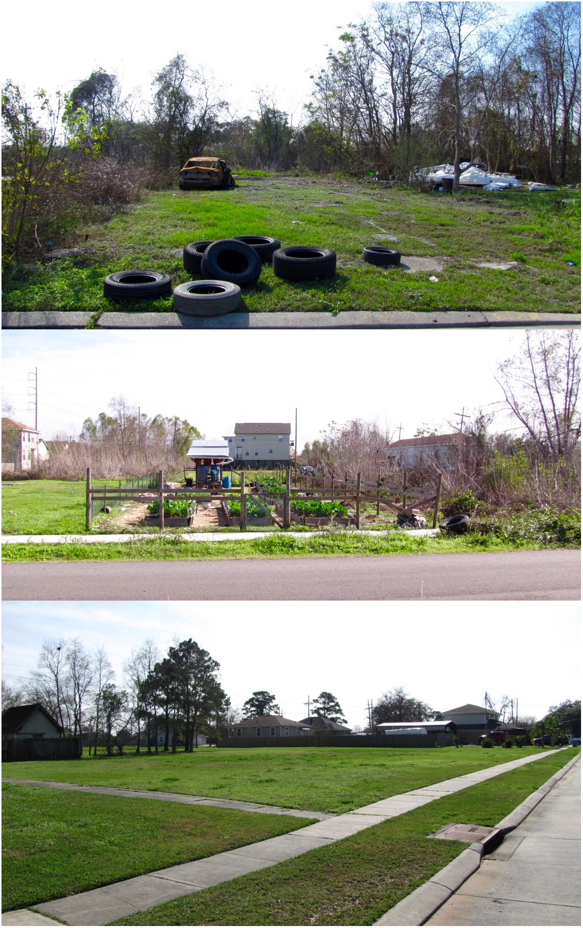
The case of post-Katrina New Orleans illustrates that who gets to decide where green space is placed, what form it takes, and who benefits from it are all influenced by social tensions, politics, and power dynamics. Marginalized communities often see the development of green space as a step toward gentrification and the eventual destruction of their community. For example, in Chicago, city leaders championed the development of the 606 Trail, a greenway created out of an unused elevated railway line. But local residents of the mostly Hispanic communities in which the new park would be built were less enthused. They feared the park would raise rents and change the cultural and racial makeup of their communities as wealthier and whiter residents moved in. Their concerns were largely ignored, and the 606 Trail has been a source of conflict ever since it was built. Indeed, many of the fears that locals had have come true. The trail has spurred a luxury real estate boom in the adjacent neighborhoods, with old rentals demolished to make way for high-end condos.200 There is some evidence that how the green space is designed can influence the degree of gentrification it spawns. Linear greenways—particularly ones located near the city center—are strong drivers of gentrification, perhaps because they provide lots of opportunities for high-end park adjacent real estate. But large parks located far from the city center aren’t associated with gentrification much if at all.201 Probably more important than the design specifics is the need to ensure that local people—particularly those who are the least powerful and socially connected members of society—are empowered to develop solutions that meet their needs and desires.
Chapter Summary
Metropolis
Most of our interaction with the Earth System now takes place in or is meditated through cities. The unique physical characteristics of cities as well as our management of urban environments affect the physiology and behavior of organisms, shape their life history, and create uniquely urban patterns of biodiversity. A better understanding of how cities function as ecosystems will help us design more ecologically sustainable and livable cities.
- Cities are dominated by hardscape that sprawls across the landscape (Figure 8.2). The sprawl fragments habitat (Figure 8.4) and creates abrupt ecotones along a wildland-urban interface (Figure 8.5). Cities also act as important resource junctions in the Earth System.
- Compared to rural areas, urban areas are warmer (Figure 8.7), generate more surface runoff (Figure 8.8), are brighter (Figure 8.3), and are louder (Figure 8.9).
- Urban domesticated landscapes reflect human social factors. These human factors have created landscapes that: have high local species richness but low regional species turnover; are greener and more diverse in wealthier than in poorer neighborhoods (Figure 8.10); have novel functional traits and species associations (Figure 8.11)
- Urban domesticated animals can act as significant pathways for the transmission of zoonotic diseases and be major predators in urban environments (Figure 8.12).
- Some non-domesticated species have adapted to urban conditions, have learned to exploit resources found in urban environments (Figure 8.13), or persist as relict populations (Figures 8.4, 8.6).
- Improving the resource and land use efficiency of cities can lessen their ecological impact. Techniques include designing more energy efficient buildings, using more precise landscape irrigation and nutrient delivery systems, using functional plant forms that are better matched to local climate (Figure 8.14), designing landscapes that leverage resource complementarity, facilitation, and functional trait uniqueness (Figure 8.15), creating denser and less sprawling urbanized land use (Figure 8.16), and creating more circular resource flows between urban and rural areas.
- We can enhance the ecosystem services that urban environments provide by creating functional green infrastructure (Table 8.2, Figures 8.17, 8.18) and more generally increasing the functional diversity of urban landscapes so that they provide a broad portfolio of ecosystem services (Table 8.3, Figure 8.22).
- We can mitigate the negative effects of urban sprawl by providing dispersal and migration pathways through urban landscapes (Figures 8.24, 8.25) and by creating habitat buffers along urban margins and the urban-wildland interface (Figures 8.27, 8.28).
- We need to design cities that more equitably deliver ecosystem services to their residents.
Additional Resources
- This global light pollution map is spatially detailed and interactive: https://www.lightpollutionmap.info.
- Read this story about the interaction between migrating birds and the Tribute in Light commemoration of September 11. It includes a brief video: Lights Dramatic Impact on Bird Migration.
- A webinar about how songbirds have adapted to the unique soundscape of cities: YouTube
- The short film Ten Parks That Changed America describes the history of 10 influential park designs and the social contexts that shaped them: 10 Parks that Changed America
References
75Aaronson, D., Faber, J., Hartley, D., Mazumder, B., Sharkey, P., 2021. The long-run effects of the 1930s HOLC “redlining” maps on place-based measures of economic opportunity and socioeconomic success. Reg. Sci. Urban Econ. 86, 103622. https://doi.org/10.1016/j.regsciurbeco.2020.103622
134Akbari, H., Kolokotsa, D., 2016. Three decades of urban heat islands and mitigation technologies research. Energy Build. 133, 834–42. https://doi.org/10.1016/j.enbuild.2016.09.067
58Alfred, R., 2010. Aug. 26, 1883: Krakatau erupts, changes world . . . again. Wired, August 26, 2010. https://www.wired.com/2010/08/0826krakatau-krakatoa-explodes/.
40Altermatt, F., Ebert, D., 2016. Reduced flight-to-light behaviour of moth populations exposed to long-term urban light pollution. Biol. Lett. 12, 20160111. https://doi.org/10.1098/rsbl.2016.0111
180Arellano, G., 2022. Heed the warnings of this palm tree, a 200-year-old drought survivor. Los Angeles Times, May 13, 2022.
82Aronson, M.F., Lepczyk, C.A., Evans, K.L., Goddard, M.A., Lerman, S.B., MacIvor, J.S., Nilon, C.H., Vargo, T., 2017. Biodiversity in the city: key challenges for urban green space management. Front. Ecol. Environ. 15, 189–96. https://doi.org/10.1002/fee.1480
93Baisden, E.C., Tallamy, D.W., Narango, D.L., Boyle, E., 2018. Do cultivars of native plants support insect herbivores? HortTechnology 28, 596–606. https://doi.org/10.21273/HORTTECH03957-18
*Baker, A.M., Redmond, C.T., Malcolm, S.B., Potter, D.A., 2020. Suitability of native milkweed (Asclepias) species versus cultivars for supporting monarch butterflies and bees in urban gardens. PeerJ 8, e9823. https://doi.org/10.7717/peerj.9823
14Balch, J.K., Bradley, B.A., Abatzoglou, J.T., Nagy, R.C., Fusco, E.J., Mahood, A.L., 2017. Human-started wildfires expand the fire niche across the United States. Proc. Natl. Acad. Sci. 114, 2946–51. https://doi.org/10.1073/pnas.1617394114
154Barnes, M.R., Nelson, K.C., Meyer, A.J., Watkins, E., Bonos, S.A., Horgan, B.P., Meyer, W.A., Murphy, J., Yue, C., 2018. Public land managers and sustainable urban vegetation: the case of low-input turfgrasses. Urban For. Urban Green. 29, 284–92. https://doi.org/10.1016/j.ufug.2017.12.008
65Basner, M., Babisch, W., Davis, A., Brink, M., Clark, C., Janssen, S., Stansfeld, S., 2014. Auditory and non-auditory effects of noise on health. The Lancet 383, 1325–32. https://doi.org/10.1016/S0140-6736(13)61613-X
117Bateman, P.W., Fleming, P.A., 2012. Big city life: carnivores in urban environments. J. Zool. 287, 1–23. https://doi.org/10.1111/j.1469-7998.2011.00887.x
10Baxter-Gilbert, J.H., Riley, J.L., Neufeld, C.J.H., Litzgus, J.D., Lesbarrères, D., 2015. Road mortality potentially responsible for billions of pollinating insect deaths annually. J. Insect Conserv. 19, 1029–35. https://doi.org/10.1007/s10841-015-9808-z
95Belsky, J., Joshi, N.K., 2018. Assessing role of major drivers in recent decline of monarch butterfly population in North America. Front. Environ. Sci. 6.
57Bennie, J., Davies, T.W., Cruse, D., Inger, R., Gaston, K.J., 2018. Artificial light at night causes top-down and bottom-up trophic effects on invertebrate populations. J. Appl. Ecol. 55, 2698–706. https://doi.org/10.1111/1365-2664.13240
11Benson, J.F., Mahoney, P.J., Vickers, T.W., Sikich, J.A., Beier, P., Riley, S.P.D., Ernest, H.B., Boyce, W.M., 2019. Extinction vortex dynamics of top predators isolated by urbanization. Ecol. Appl. 29, e01868. https://doi.org/10.1002/eap.1868
1Bettencourt, L.M.A., Lobo, J., Helbing, D., Kühnert, C., West, G.B., 2007. Growth, innovation, scaling, and the pace of life in cities. Proc. Natl. Acad. Sci. 104, 7301–6. https://doi.org/10.1073/pnas.0610172104
47Bird, B.L., Branch, L.C., Miller, D.L., 2004. Effects of coastal lighting on foraging behavior of beach mice. Conserv. Biol. 18, 1435–39. https://doi.org/10.1111/j.1523-1739.2004.00349.x
200Black, C., 2020. “Green gentrification” and lessons of the 606. Chicago Reporter, January 30, 2020.
126Bókony, V., Üveges, B., Verebélyi, V., Ujhegyi, N., Móricz, Á.M., 2019. Toads phenotypically adjust their chemical defences to anthropogenic habitat change. Sci. Rep. 9, 3163. https://doi.org/10.1038/s41598-019-39587-3
70Bormann, F.H., Balmori, D., Geballe, G.T., 2001. Redesigning the American Lawn: A Search for Environmental Harmony. New Haven, CT: Yale University Press.
143Botías, C., David, A., Hill, E.M., Goulson, D., 2017. Quantifying exposure of wild bumblebees to mixtures of agrochemicals in agricultural and urban landscapes. Environ. Pollut. 222, 73–82. https://doi.org/10.1016/j.envpol.2017.01.001
120Braczkowski, A.R., O’Bryan, C.J., Stringer, M.J., Watson, J.E., Possingham, H.P., Beyer, H.L., 2018. Leopards provide public health benefits in Mumbai, India. Front. Ecol. Environ. 16, 176–82. https://doi.org/10.1002/fee.1776
121Breck, S.W., Poessel, S.A., Mahoney, P., Young, J.K., 2019. The intrepid urban coyote: a comparison of bold and exploratory behavior in coyotes from urban and rural environments. Sci. Rep. 9, 2104. https://doi.org/10.1038/s41598-019-38543-5
37Browne, M.A., Underwood, A.J., Chapman, M.G., Williams, R., Thompson, R.C., van Franeker, J.A., 2015. Linking effects of anthropogenic debris to ecological impacts. Proc. R. Soc. B Biol. Sci. 282, 20142929. https://doi.org/10.1098/rspb.2014.2929
59Buxton, R.T., McKenna, M.F., Mennitt, D., Fristrup, K., Crooks, K., Angeloni, L., Wittemyer, G., 2017. Noise pollution is pervasive in U.S. protected areas. Science 356, 531–33. https://doi.org/10.1126/science.aah4783
44Cabrera-Cruz, S.A., Smolinsky, J.A., Buler, J.J., 2018. Light pollution is greatest within migration passage areas for nocturnally-migrating birds around the world. Sci. Rep. 8, 3261. https://doi.org/10.1038/s41598-018-21577-6
181Carroll, R., 2017. Los Angeles’ legendary palm trees are dying—and few will be replaced. The Guardian, September 29, 2017.
54Chang, A.-M., Aeschbach, D., Duffy, J.F., Czeisler, C.A., 2015. Evening use of light-emitting eReaders negatively affects sleep, circadian timing, and next-morning alertness. Proc. Natl. Acad. Sci. 112, 1232–37. https://doi.org/10.1073/pnas.1418490112
33Chick, L.D., Strickler, S.A., Perez, A., Martin, R.A., Diamond, S.E., 2019. Urban heat islands advance the timing of reproduction in a social insect. J. Therm. Biol. 80, 119–25. https://doi.org/10.1016/j.jtherbio.2019.01.004
90Cohen, H., Philpott, S.M., Liere, H., Lin, B.B., Jha, S., 2021. The relationship between pollinator community and pollination services is mediated by floral abundance in urban landscapes. Urban Ecosyst. 24, 275–90. https://doi.org/10.1007/s11252-020-01024-z
182Colding, J., Folke, C., 2009. The role of golf courses in biodiversity conservation and ecosystem management. Ecosystems 12, 191–206. https://doi.org/10.1007/s10021-008-9217-1
Combs, M., Puckett, E.E., Richardson, J., Mims, D., Munshi-South, J., 2018. Spatial population genomics of the brown rat (Rattus norvegicus) in New York City. Mol. Ecol. 27, 83–98. https://doi.org/10.1111/mec.14437
152Cook, E.M., Hall, S.J., Larson, K.L., 2012. Residential landscapes as social-ecological systems: a synthesis of multi-scalar interactions between people and their home environment. Urban Ecosyst. 15, 19–52. https://doi.org/10.1007/s11252-011-0197-0
92Corbet, S.A., Bee, J., Dasmahapatra, K., Gale, S., Gorringe, E., La Ferla, B., Moorhouse, T., Trevail, A., Van Bergen, Y., Vorontsova, M., 2001. Native or exotic? Double or single? Evaluating plants for pollinator-friendly gardens. Ann. Bot. 87, 219–32. https://doi.org/10.1006/anbo.2000.1322
12Cuwen, T., 2017. A week in the life of P-22, the big cat who shares Griffith Park with millions of people. Los Angeles Times, February 8, 2017.
79Davoren, E., 2017. Plant diversity patterns of domestic gardens in five settlements of South Africa (doctoral thesis). Potchefstroom Campus, North-West University.
189Denneboom, D., Bar-Massada, A., Shwartz, A., 2021. Factors affecting usage of crossing structures by wildlife—a systematic review and meta-analysis. Sci. Total Environ. 777, 146061. https://doi.org/10.1016/j.scitotenv.2021.146061
133Dimovski, A.M., Robert, K.A., 2018. Artificial light pollution: shifting spectral wavelengths to mitigate physiological and health consequences in a nocturnal marsupial mammal. J. Exp. Zool. Part Ecol. Integr. Physiol. 329, 497–505. https://doi.org/10.1002/jez.2163
45Doren, B.M.V., Horton, K.G., Dokter, A.M., Klinck, H., Elbin, S.B., Farnsworth, A., 2017. High-intensity urban light installation dramatically alters nocturnal bird migration. Proc. Natl. Acad. Sci. 114, 11,175–80. https://doi.org/10.1073/pnas.1708574114
20Drechsel, P., Graefe, S., Fink, M., 2007. Rural-Urban Food, Nutrient and Virtual Water Flows in Selected West African Cities. Colombo, Sri Lanka: International Water Management Institute.
151Dukes, M.D., 2012. Water conservation potential of landscape irrigation smart controllers. Trans. ASABE 55, 563–69.
6Elhacham, E., Ben-Uri, L., Grozovski, J., Bar-On, Y.M., Milo, R., 2020. Global human-made mass exceeds all living biomass. Nature 588, 442–44. https://doi.org/10.1038/s41586-020-3010-5
7Ellis, E.C., Ramankutty, N., 2008. Putting people in the map: anthropogenic biomes of the world. Front. Ecol. Environ. 6, 439–47. https://doi.org/10.1890/070062
*Elvidge, C.D., Tuttle, B.T., Sutton, P.C., Baugh, K.E., Howard, A.T., Milesi, C., Bhaduri, B., Nemani, R., 2007. Global distribution and density of constructed impervious surfaces. Sensors 7, 1962–79. https://doi.org/10.3390/s7091962
*Entrix, Inc., 2010. Portland’s Green Infrastructure: Quantifying the Health, Energy, and Community Livability Benefits. Portland, Oregon: Bureau of Environmental Services.
**Erickson, E., Patch, H.M., Grozinger, C.M., 2021. Herbaceous perennial ornamental plants can support complex pollinator communities. Sci. Rep. 11, 17352. https://doi.org/10.1038/s41598-021-95892-w
119Everingham, S.E., Hemmings, F., Moles, A.T., 2019. Inverted invasions: native plants can frequently colonise urban and highly disturbed habitats. Austral Ecol. 0. https://doi.org/10.1111/aec.12719
39Falchi, F., Cinzano, P., Duriscoe, D., Kyba, C.C.M., Elvidge, C.D., Baugh, K., Portnov, B.A., Rybnikova, N.A., Furgoni, R., 2016. The new world atlas of artificial night sky brightness. Sci. Adv. 2, e1600377. https://doi.org/10.1126/sciadv.1600377
135Falk, J.H., 1976. Energetics of a suburban lawn ecosystem. Ecology 57, 141–50. https://doi.org/10.2307/1936405
174Filazzola, A., Shrestha, N., MacIvor, J.S., 2019. The contribution of constructed green infrastructure to urban biodiversity: a synthesis and meta-analysis. J. Appl. Ecol. 56, 2131–43. https://doi.org/10.1111/1365-2664.13475
29Founda, D., Santamouris, M., 2017. Synergies between urban heat island and heat waves in Athens (Greece), during an extremely hot summer (2012). Sci. Rep. 7, 10973. https://doi.org/10.1038/s41598-017-11407-6
2Friedlander, D., 1970. The spread of urbanization in England and Wales, 1851-1951. Popul. Stud. 24, 423–43. https://doi.org/10.2307/2173046
66Fritschi, L., Brown, A., Kim, R., Kephalapoulos, S. (Eds.), 2011. Burden of Disease from Environmental Noise. Bonn: World Health Organization.
192Fry, H., Reyes-Velarde, A., 2019. California wastes most of its rainwater, which simply goes down the drain. Los Angeles Times, February 20, 2019.
196Garrison, J.D., 2019. Seeing the park for the trees: New York’s “Million Trees” campaign vs. the deep roots of environmental inequality. Environ. Plan. B Urban Anal. City Sci. 46, 914–30. https://doi.org/10.1177/2399808317737071
53Gaston, K.J., Bennie, J., Davies, T.W., Hopkins, J., 2013. The ecological impacts of nighttime light pollution: a mechanistic appraisal. Biol. Rev. 88, 912–27. https://doi.org/10.1111/brv.12036
157Gaura, E., Brusey, J.P., 2021. Nikola Tesla: 5G network could realise his dream of wireless electricity, a century after experiments failed. The Conversation, April 9, 2021. http://theconversation.com/nikola-tesla-5g-network-could-realise-his-dream-of-wireless-electricity-a-century-after-experiments-failed-158665 (accessed 5.6.22).
159Gocmen, A., 2019. Directions for environmentally sustainable residential development research in the urban-rural interface. Presented at the Workshop on Developing a Convergence Sustainable Urban Systems Agenda for Redesigning the Urban-Rural Interface along the Mississippi River Watershed, Ames, Iowa, August 12–13, 2019. https://doi.org/10.31274/3d9ea6a4.7a5bbb7b
8González‐Suárez, M., Ferreira, F.Z., Grilo, C., 2018. Spatial and species-level predictions of road mortality risk using trait data. Global Ecol. Biogeogr. 27, 1093–105. https://doi.org/10.1111/geb.12769
67Gould van Praag, C.D., Garfinkel, S.N., Sparasci, O., Mees, A., Philippides, A.O., Ware, M., Ottaviani, C., Critchley, H.D., 2017. Mind-wandering and alterations to default mode network connectivity when listening to naturalistic versus artificial sounds. Sci. Rep. 7, 45273. https://doi.org/10.1038/srep45273
71Graves, R. A., Pearson, S. M., & Turner, M. G., 2017. Species richness alone does not predict cultural ecosystem service value. Proceedings of the National Academy of Sciences, 201701370. https://doi.org/10.1073/pnas.1701370114
9Grilo, C., Koroleva, E., Andrášik, R., Bíl, M., González-Suárez, M., 2020. Roadkill risk and population vulnerability in European birds and mammals. Front. Ecol. Environ. 18, 323–28. https://doi.org/10.1002/fee.2216
38Guzy, M., Richardson, K., Lambrinos, J.G., 2015. A tool for assisting municipalities in developing riparian shade inventories. Urban For. Urban Green. 14, 345–53. https://doi.org/10.1016/j.ufug.2015.02.012
164Haghighi, E., Madani, K., Hoekstra, A.Y., 2018. The water footprint of water conservation using shade balls in California. Nat. Sustainability 1, 358. https://doi.org/10.1038/s41893-018-0092-2
99Hall, D.M., Camilo, G.R., Tonietto, R.K., Ollerton, J., Ahrné, K., Arduser, M., Ascher, J.S., Baldock, K.C.R., Fowler, R., Frankie, G., Goulson, D., Gunnarsson, B., Hanley, M.E., Jackson, J.I., Langellotto, G., Lowenstein, D., Minor, E.S., Philpott, S.M., Potts, S.G., Sirohi, M.H., Spevak, E.M., Stone, G.N., Threlfall, C.G., 2017. The city as a refuge for insect pollinators. Conserv. Biol. 31, 24–29. https://doi.org/10.1111/cobi.12840
21 Hall, S.J., Learned, J., Ruddell, B., Larson, K.L., Cavender-Bares, J., Bettez, N., Groffman, P.M., Grove, J.M., Heffernan, J.B., Hobbie, S.E., Morse, J.L., Neill, C., Nelson, K.C., O’Neil-Dunne, J.P.M., Ogden, L., Pataki, D.E., Pearse, W.D., Polsky, C., Chowdhury, R.R., Steele, M.K., Trammell, T.L.E., 2016. Convergence of microclimate in residential landscapes across diverse cities in the United States. Landscape Ecol. 31, 101–17. https://doi.org/10.1007/s10980-015-0297-y
166Herrero-Jáuregui, C., Arnaiz-Schmitz, C., Reyes, M.F., Telesnicki, M., Agramonte, I., Easdale, M.H., Schmitz, M.F., Aguiar, M., Gómez-Sal, A., Montes, C., 2018. What do we talk about when we talk about social-ecological systems? A literature review. Sustainability 10, 2950. https://doi.org/10.3390/su10082950
136Hilaire, R.S., Arnold, M.A., Wilkerson, D.C., Devitt, D.A., Hurd, B.H., Lesikar, B.J., Lohr, V.I., Martin, C.A., McDonald, G.V., Morris, R.L., Pittenger, D.R., Shaw, D.A., Zoldoske, D.F., 2008. Efficient water use in residential urban landscapes. HortScience 43, 2081–92. https://doi.org/10.21273/HORTSCI.43.7.2081
139Hobbie, S.E., Finlay, J.C., Janke, B.D., Nidzgorski, D.A., Millet, D.B., Baker, L.A., 2017. Contrasting nitrogen and phosphorus budgets in urban watersheds and implications for managing urban water pollution. Proc. Natl. Acad. Sci. 114, 4177–82. https://doi.org/10.1073/pnas.1618536114
18Hoekstra, A.Y., Mekonnen, M.M., 2012. The water footprint of humanity. Proc. Natl. Acad. Sci. 109, 3232–37. https://doi.org/10.1073/pnas.1109936109
*Hoffman, J.S., Shandas, V., Pendleton, N., 2020. The effects of historical housing policies on resident exposure to intra-urban heat: a study of 108 us urban areas. Climate 8, 12. https://doi.org/10.3390/cli8010012
272830International Energy Agency, 2018. The Future of Cooling Opportunities for Energy-Efficient Air Conditioning. Paris: International Energy Agency.
199Johannessen, M., Goldweit-Denton, D., 2020. The green dot effect: neighborhood recovery after Hurricane Katrina. Conflict Urbanism (Spring 2020).
123 Johnson, M. T. J., Prashad, C.M., Lavoignat, M., Saini, H.S., 2018. Contrasting the effects of natural selection, genetic drift and gene flow on urban evolution in white clover (Trifolium repens). Proc. R. Soc. B Biol. Sci. 285, 20181019. https://doi.org/10.1098/rspb.2018.1019
165Kabbe, C., 2015. Sustainable Sewage Sludge Management Fostering Phosphorus Recovery and Energy Efficiency: Final Report. Brussels: Seventh Framework Programme, European Commission.
105Kaminski, J., Waller, B.M., Diogo, R., Hartstone-Rose, A., Burrows, A.M., 2019. Evolution of facial muscle anatomy in dogs. Proc. Natl. Acad. Sci. 116, 14,677-81. https://doi.org/10.1073/pnas.1820653116
173Keeler, B.L., Hamel, P., McPhearson, T., Hamann, M.H., Donahue, M.L., Prado, K.A.M., Arkema, K.K., Bratman, G.N., Brauman, K.A., Finlay, J.C., Guerry, A.D., Hobbie, S.E., Johnson, J.A., MacDonald, G.K., McDonald, R.I., Neverisky, N., Wood, S.A., 2019. Social-ecological and technological factors moderate the value of urban nature. Nat. Sustainability 2, 29. https://doi.org/10.1038/s41893-018-0202-1
153Kelly, D., 2013. Pesticide blamed in death of 25,000 bumblebees in Oregon. Los Angeles Times, June 21, 2013.
118Kettel, E.F., Gentle, L.K., Yarnell, R.W., Quinn, J.L., 2019. Breeding performance of an apex predator, the peregrine falcon, across urban and rural landscapes. Urban Ecosyst. 22, 117–25. https://doi.org/10.1007/s11252-018-0799-x
72Khachatryan, H., Knuth, M., Hodges, A., Hall, C., 2021. Florida Nursery and Landscape Industry Characteristics. Report FE1108. Gainesville: Food and Resource Economics Department, University of Florida Institute of Food and Agricultural Sciences.
140Kiely, T., Donaldson, D., Grube, A., 2004. Pesticide Industry Sales and Usage: 2000 and 2001 Market Estimates. Washington, DC: US Environmental Protection Agency.
197Lamb, Z., 2020. Connecting the dots: the origins, evolutions, and implications of the map that changed post-Katrina recovery planning in New Orleans. In: Laska, S. (Ed.), Louisiana’s Response to Extreme Weather: A Coastal State’s Adaptation Challenges and Successes, Extreme Weather and Society. Cham, Switzerland: Springer International, 65–91. https://doi.org/10.1007/978-3-030-27205-0_3
167Lambrinos, J.G., 2015. Water through green roofs. In: Sutton, R.K. (Ed.), Green Roof Ecosystems, Ecological Studies. Cham, Switzerland: Springer International, 81–105. https://doi.org/10.1007/978-3-319-14983-7_4
155Larsen, L., Harlan, S.L., 2006. Desert dreamscapes: residential landscape preference and behavior. Landscape Urban Plan. 78, 85–100. https://doi.org/10.1016/j.landurbplan.2005.06.002
137Law, N., Band, L., Grove, M., 2004. Nitrogen input from residential lawn care practices in suburban watersheds in Baltimore County, MD. J. Environ. Plan. Manage. 47, 737–55. https://doi.org/10.1080/0964056042000274452
110Legge, S., Woinarski, J.C.Z., Dickman, C.R., Murphy, B.P., Woolley, L.-A., Calver, M.C., Legge, S., Woinarski, J.C.Z., Dickman, C.R., Murphy, B.P., Woolley, L.-A., Calver, M.C., 2020. We need to worry about Bella and Charlie: the impacts of pet cats on Australian wildlife. Wildl. Res. 47, 523–39. https://doi.org/10.1071/WR19174
*Lehigh Valley Planning Commission, 2015. Model Ordinance: Conservation Subdivisions. Allentown, PA: Lehigh Valley Planning Commission.
73Leong, M., Dunn, R.R., Trautwein, M.D., 2018. Biodiversity and socioeconomics in the city: a review of the luxury effect. Biol. Lett. 14, 20180082. https://doi.org/10.1098/rsbl.2018.0082
87Lerman, S.B., Contosta, A.R., Milam, J., Bang, C., 2018. To mow or to mow less: lawn mowing frequency affects bee abundance and diversity in suburban yards. Biol. Conserv. 221, 160–74. https://doi.org/10.1016/j.biocon.2018.01.025
*198Lewis, J.A., Zipperer, W.C., Ernstson, H., Bernik, B., Hazen, R., Elmqvist, T., Blum, M.J., 2017. Socioecological disparities in New Orleans following Hurricane Katrina. Ecosphere 8, e01922. https://doi.org/10.1002/ecs2.1922
169Liberalesso, T., Oliveira Cruz, C., Matos Silva, C., Manso, M., 2020. Green infrastructure and public policies: an international review of green roofs and green walls incentives. Land Use Policy 96, 104693. https://doi.org/10.1016/j.landusepol.2020.104693
184Lindemann-Matthies, P., Mulyk, L., Remmele, M., 2021. Garden plants for wild bees—laypersons’ assessment of their suitability and opinions on gardening approaches. Urban For. Urban Green. 62, 127181. https://doi.org/10.1016/j.ufug.2021.127181
191Lloyd, A., 2017. A brief history of LA’s Indigenous Tongva people. LAist, October 8, 2017.
76Locke, D.H., Hall, B., Grove, J.M., Pickett, S.T.A., Ogden, L.A., Aoki, C., Boone, C.G., O’Neil-Dunne, J.P.M., 2021. Residential housing segregation and urban tree canopy in 37 US Cities. Npj Urban Sustainability 1, 1–9. https://doi.org/10.1038/s42949-021-00022-0
108Loss, S.R., Marra, P.P., 2017. Population impacts of free-ranging domestic cats on mainland vertebrates. Front. Ecol. Environ. 15, 502–9. https://doi.org/10.1002/fee.1633
107 Loss, S.R., Will, T., Marra, P.P., 2013. The impact of free-ranging domestic cats on wildlife of the United States. Nat. Commun. 4, 1396. https://doi.org/10.1038/ncomms2380
43Loss, S.R., Will, T., Loss, S.S., Marra, P.P., 2014. Bird–building collisions in the United States: estimates of annual mortality and species vulnerability. The Condor 116, 8–23. https://doi.org/10.1650/CONDOR-13-090.1
41Loss, S.R., Will, T., Marra, P.P., 2015. Direct mortality of birds from anthropogenic causes. Annu. Rev. Ecol. Evol. Syst. 46, 99–120. https://doi.org/10.1146/annurev-ecolsys-112414-054133
>em class=”figure-11″>109Loss, S.R., Will, T., Longcore, T., Marra, P.P., 2018. Responding to misinformation and criticisms regarding United States cat predation estimates. Biol. Invasions 20, 3385–96. https://doi.org/10.1007/s10530-018-1796-y
50Ludvigsen, M., Berge, J., Geoffroy, M., Cohen, J.H., Torre, P.R.D.L., Nornes, S.M., Singh, H., Sørensen, A.J., Daase, M., Johnsen, G., 2018. Use of an autonomous surface vehicle reveals small-scale diel vertical migrations of zooplankton and susceptibility to light pollution under low solar irradiance. Sci. Adv. 4, eaap9887. https://doi.org/10.1126/sciadv.aap9887
63Luo, J., Siemers, B.M., Koselj, K., 2015. How anthropogenic noise affects foraging. Global Change Biol. 21, 3278–89. https://doi.org/10.1111/gcb.12997
103Ma, W., Kahn, R.E., Richt, J.A., 2008. The pig as a mixing vessel for influenza viruses: human and veterinary implications. J. Mol. Genet. Med. 3, 158–66.
42Machtans, C., Wedeles, C., Bayne, E., 2013. A first estimate for Canada of the number of birds killed by colliding with building windows. Avian Conserv. Ecol. 8. https://doi.org/10.5751/ACE-00568-080206
13Mann, M.L., Batllori, E., Moritz, M.A., Waller, E.K., Berck, P., Flint, A.L., Flint, L.E., Dolfi, E., 2016. Incorporating anthropogenic influences into fire probability models: effects of human activity and climate change on fire activity in California. PLoS One 11, e0153589. https://doi.org/10.1371/journal.pone.0153589
170Manso, M., Teotónio, I., Silva, C.M., Cruz, C.O., 2021. Green roof and green wall benefits and costs: a review of the quantitative evidence. Renewable Sustainable Energy Rev. 135, 110111. https://doi.org/10.1016/j.rser.2020.110111
138Maryland Department of Agriculture, 2009. Maryland Nutrient Management Manual. Annapolis: Maryland Department of Agriculture.
100Matteson, K.C., Ascher, J.S., Langellotto, G.A., 2008. Bee richness and abundance in New York City urban gardens. Ann. Entomol. Soc. Am. 101, 140–50. https://doi.org/10.1603/0013-8746(2008)101[140:BRAAIN]2.0.CO;2
102Maxmen, A., 2022. Wuhan market was epicentre of pandemic’s start, studies suggest. Nature 603, 15–16. https://doi.org/10.1038/d41586-022-00584-8
80Mazumdar, S., Mazumdar, S., 2012. Immigrant home gardens: places of religion, culture, ecology, and family. Landscape Urban Plan. 105, 258–65. https://doi.org/10.1016/j.landurbplan.2011.12.020
36McGrane, S.J., 2016. Impacts of urbanisation on hydrological and water quality dynamics, and urban water management: a review. Hydrol. Sci. J. 61, 2295–311. https://doi.org/10.1080/02626667.2015.1128084
163McKuin, B., Zumkehr, A., Ta, J., Bales, R., Viers, J.H., Pathak, T., Campbell, J.E., 2021. Energy and water co-benefits from covering canals with solar panels. Nat. Sustainability 4, 609–17. https://doi.org/10.1038/s41893-021-00693-8
34Meng, L., Mao, J., Zhou, Y., Richardson, A.D., Lee, X., Thornton, P.E., Ricciuto, D.M., Li, X., Dai, Y., Shi, X., Jia, G., 2020. Urban warming advances spring phenology but reduces the response of phenology to temperature in the conterminous United States. Proc. Natl. Acad. Sci. 117, 4228–33. https://doi.org/10.1073/pnas.1911117117
19Metson, G.S., Bennett, E.M., 2015. Phosphorus cycling in Montreal’s food and urban agriculture systems. PLoS One 10, e0120726. https://doi.org/10.1371/journal.pone.0120726
49Meyer, L.A., Sullivan, S.M.P., 2013. Bright lights, big city: influences of ecological light pollution on reciprocal stream–riparian invertebrate fluxes. Ecol. Appl. 23, 1322–30. https://doi.org/10.1890/12-2007.1
122Miles, L.S., Carlen, E.J., Winchell, K.M., Johnson, M.T.J., 2021. Urban evolution comes into its own: emerging themes and future directions of a burgeoning field. Evol. Appl. 14, 3–11. https://doi.org/10.1111/eva.13165
131Miller, S.A., John, V.M., Pacca, S.A., Horvath, A., 2018. Carbon dioxide reduction potential in the global cement industry by 2050. Cem. Concr. Res. 114, 115–24. https://doi.org/10.1016/j.cemconres.2017.08.026
85Muratet, A., Fontaine, B., 2015. Contrasting impacts of pesticides on butterflies and bumblebees in private gardens in France. Biol. Conserv. 182, 148–54. https://doi.org/10.1016/j.biocon.2014.11.045
97Narango, D.L., Tallamy, D.W., Marra, P.P., 2018. Nonnative plants reduce population growth of an insectivorous bird. Proc. Natl. Acad. Sci. 115, 11,549–54. https://doi.org/10.1073/pnas.1809259115
78Nardone, A., Casey, J.A., Morello-Frosch, R., Mujahid, M., Balmes, J.R., Thakur, N., 2020. Associations between historical residential redlining and current age-adjusted rates of emergency department visits due to asthma across eight cities in California: an ecological study. Lancet Planet. Health 4, e24–e31. https://doi.org/10.1016/S2542-5196(19)30241-4
77Nardone, A., Rudolph, K.E., Morello-Frosch, R., Casey, J.A., 2021. Redlines and greenspace: the relationship between historical redlining and 2010 greenspace across the United States. Environ. Health Perspect. 129, 017006. https://doi.org/10.1289/EHP7495
129National Park Service, 2002. Santa Monica Mountains National Recreation Area California General Management Plant Environmental Impact Statement. Washington, DC: US Department of the Interior.
171Netusil, N.R., Lavelle, L., Dissanayake, S., Ando, A.W., 2022. Valuing the public benefits of green roofs. Landscape Urban Plan. 224, 104426. https://doi.org/10.1016/j.landurbplan.2022.104426
114Newsome, T.M., Van Eeden, L.M., 2017. The effects of food waste on wildlife and humans. Sustainability 9, 1269. https://doi.org/10.3390/su9071269
52Nordt, A., Klenke, R., 2013. Sleepless in town—drivers of the temporal shift in dawn song in urban European Blackbirds. PLoS One 8, e71476. https://doi.org/10.1371/journal.pone.0071476
178Nowak, D.J., Greenfield, E.J., 2018. Declining urban and community tree cover in the United States. Urban For. Urban Green. 32, 32–55. https://doi.org/10.1016/j.ufug.2018.03.006
158Oregon Metro, 2020. Urban growth boundary. Last published February 24, 2020, https://www.oregonmetro.gov/urban-growth-boundary.
146Osmond, D.L., Hardy, D.H., 2004. Characterization of turf practices in five North Carolina communities. J. Environ. Qual. 33, 565–75. https://doi.org/10.2134/jeq2004.5650
89Otoshi, M.D., Bichier, P., Philpott, S.M., 2015. Local and landscape correlates of spider activity density and species richness in urban gardens. Environ. Entomol. 44, 1043–51. https://doi.org/10.1093/ee/nvv098
55Ouyang, J.Q., Davies, S., Dominoni, D., 2018. Hormonally mediated effects of artificial light at night on behavior and fitness: linking endocrine mechanisms with function. J. Exp. Biol. 221, jeb156893. https://doi.org/10.1242/jeb.156893
128Palta, M.M., Grimm, N.B., Groffman, P.M., 2017. “Accidental” urban wetlands: ecosystem functions in unexpected places. Front. Ecol. Environ. 15, 248–56. https://doi.org/10.1002/fee.1494
112Panagiotakopuli, E., Buckland, P.C., 1999. Cimex lectularius L., the common bed bug from Pharaonic Egypt. Antiquity 73, 908.
179Pataki, D.E., Alberti, M., Cadenasso, M.L., Felson, A.J., McDonnell, M.J., Pincetl, S., Pouyat, R.V., Setälä, H., Whitlow, T.H., 2021. The benefits and limits of urban tree planting for environmental and human health. Front. Ecol. Evol. 9.
185Pawelek, J.C., Frankie, G.W., Frey, K., Guerrero, S.L., Schindler, M., 2015. California Bee-Friendly Garden Recipes. ANR Publication 8518. Davis: Agriculture and Natural Resources, University of California. https://doi.org/10.3733/ucanr.8518
193 PBL Netherlands Environmental Assessment Agency [WWW Document], n.d. Low probabilities – large consequences. Reducing the vulnerability of the Dutch population to floods. URL https://themasites.pbl.nl/flood-risks/ (accessed 10.17.22).
91Pearse, W.D., Cavender‐Bares, J., Hobbie, S.E., Avolio, M.L., Bettez, N., Chowdhury, R.R., Darling, L.E., Groffman, P.M., Grove, J.M., Hall, S.J., Heffernan, J.B., Learned, J., Neill, C., Nelson, K.C., Pataki, D.E., Ruddell, B.L., Steele, M.K., Trammell, T.L.E., 2018. Homogenization of plant diversity, composition, and structure in North American urban yards. Ecosphere 9, e02105. https://doi.org/10.1002/ecs2.2105
68Peng, C., Zhao, X., Liu, G., 2015. Noise in the sea and its impacts on marine organisms. Int. J. Environ. Res. Public. Health 12, 12,304–23. https://doi.org/10.3390/ijerph121012304
98Pétremand, G., Chittaro, Y., Braaker, S., Brenneisen, S., Gerner, M., Obrist, M.K., Rochefort, S., Szallies, A., Moretti, M., 2018. Ground beetle (Coleoptera: Carabidae) communities on green roofs in Switzerland: synthesis and perspectives. Urban Ecosyst. 21, 119–32. https://doi.org/10.1007/s11252-017-0697-7
156Pincetl, S., Gillespie, T.W., Pataki, D.E., Porse, E., Jia, S., Kidera, E., Nobles, N., Rodriguez, J., Choi, D., 2019. Evaluating the effects of turf-replacement programs in Los Angeles. Landscape Urban Plan. 185, 210–21. https://doi.org/10.1016/j.landurbplan.2019.01.011
104Plowright, R.K., Foley, P., Field, H.E., Dobson, A.P., Foley, J.E., Eby, P., Daszak, P., 2011. Urban habituation, ecological connectivity and epidemic dampening: the emergence of Hendra virus from flying foxes (Pteropus spp.). Proc. R. Soc. B Biol. Sci. 278, 3703–12. https://doi.org/10.1098/rspb.2011.0522
83 Politi Bertoncini, A., Machon, N., Pavoine, S., Muratet, A., 2012. Local gardening practices shape urban lawn floristic communities. Landscape Urban Plan. 105, 53–61. https://doi.org/10.1016/j.landurbplan.2011.11.017
64Potvin, D.A., 2017. Coping with a changing soundscape: avoidance, adjustments and adaptations. Anim. Cogn. 20, 9–18. https://doi.org/10.1007/s10071-016-0999-9
116Prendergast, K.S., Dixon, K.W., Bateman, P.W., 2022. A global review of determinants of native bee assemblages in urbanised landscapes. Insect Conserv. Diversity 15, 385-405. https://doi.org/10.1111/icad.12569
Puckett, E., Jane, P., Combs, M., Blum, M.J., Bryant, J.E., Caccone, A., Costa, F., Deinum, E.E., Esther, A., Himsworth, C.G., Keightley, P.D., Ko, A., Lundkvist, Å., McElhinney, L.M., Morand, S., Robins, J., Russell, J., Strand, T.M., Suarez, O., Yon, L., Munshi-South, J., 2016. Global population divergence and admixture of the brown rat (Rattus norvegicus). Proc. R. Soc. B Biol. Sci. 283, 20161762. https://doi.org/10.1098/rspb.2016.1762
16Radeloff, V.C., Helmers, D.P., Kramer, H.A., Mockrin, M.H., Alexandre, P.M., Bar-Massada, A., Butsic, V., Hawbaker, T.J., Martinuzzi, S., Syphard, A.D., Stewart, S.I., 2018. Rapid growth of the US wildland-urban interface raises wildfire risk. Proc. Natl. Acad. Sci. 115, 3314–19. https://doi.org/10.1073/pnas.1718850115
187Ramalho, C.E., Ottewell, K.M., Chambers, B.K., Yates, C.J., Wilson, B.A., Bencini, R., Barrett, G., 2018. Demographic and genetic viability of a medium-sized ground-dwelling mammal in a fire prone, rapidly urbanizing landscape. PLoS One 13, e0191190. https://doi.org/10.1371/journal.pone.0191190
31Reese, A., 2018. As countries crank up the AC, emissions of potent greenhouse gases are likely to skyrocket. Science 359, 1084.
201Rigolon, A., Németh, J., 2020. Green gentrification or “just green enough”: do park location, size and function affect whether a place gentrifies or not? Urban Stud. 57, 402–20. https://doi.org/10.1177/0042098019849380
162Rupiper, A., Weill, J., Bruno, E., Jessoe, K., Loge, F., 2022. Untapped potential: leak reduction is the most cost-effective urban water management tool. Environ. Res. Lett. 17, 034021. https://doi.org/10.1088/1748-9326/ac54cb
115Rydell, J., 1991. Seasonal use of illuminated areas by foraging northern bats Eptesicus nilssoni. Ecography 14, 203–7. https://doi.org/10.1111/j.1600-0587.1991.tb00653.x
132Saadeh, S., Ralla, A., Al-Zubi, Y., Wu, R., Harvey, J., 2019. Application of fully permeable pavements as a sustainable approach for mitigation of stormwater runoff. Int. J. Transp. Sci. Technol. 8, 338-350. https://doi.org/10.1016/j.ijtst.2019.02.001
188Sahagún, L., 2022. A cougar passage rises over a deadly Southern California freeway. Los Angeles Times, April 22, 2022.
106Samson, M.-I., 2019. The urban metabolism of the Greater Toronto Area: a study of nitrogen and phosphorus fluxes across the urban, suburban, and rural continuum (doctoral thesis). University of Waterloo .
190Sawaya, M. A., Clevenger, A. P., & Kalinowski, S. T., 2013. Demographic connectivity for ursid populations at wildlife crossing structures in Banff National Park. Conservation Biology, 27(4), 721–730. https://doi.org/10.1111/cobi.12075
74Schell, C.J., Dyson, K., Fuentes, T.L., Des Roches, S., Harris, N.C., Miller, D.S., Woelfle-Erskine, C.A., Lambert, M.R., 2020. The ecological and evolutionary consequences of systemic racism in urban environments. Science 369, eaay4497. https://doi.org/10.1126/science.aay4497
172Schultz, I., Sailor, D.J., Starry, O., 2018. Effects of substrate depth and precipitation characteristics on stormwater retention by two green roofs in Portland OR. J. Hydrol. Reg. Stud. 18, 110–18. https://doi.org/10.1016/j.ejrh.2018.06.008
127Sebold, K.R., Leach, S.A., 1991. Historic Themes and Resources within the New Jersey Coastal Heritage Trail Route: Southern New Jersey and the Delaware Bay: Cape May, Cumberland, and Salem Counties. Historic American Buildings Survey/Historic American Engineering Record. Washington, DC: US Department of the Interior, National Park Service.
25Shepherd, J.M., 2005. A review of current investigations of urban-induced rainfall and recommendations for the future. Earth Interact. 9, 1–27. https://doi.org/10.1175/EI156.1
24 Shepherd, J.M., Pierce, H., Negri, A.J., 2002. Rainfall modification by major urban areas: observations from spaceborne rain radar on the TRMM Satellite. J. Appl. Meteorol. 41, 689–701. https://doi.org/10.1175/1520-0450(2002)041<0689:RMBMUA>2.0.CO;2
62Siemers, B.M., Schaub, A., 2011. Hunting at the highway: traffic noise reduces foraging efficiency in acoustic predators. Proc. R. Soc. B Biol. Sci. 278, 1646–52. https://doi.org/10.1098/rspb.2010.2262
*Sierro, J., Schloesing, E., Pavón, I., Gil, D., 2017. European blackbirds exposed to aircraft noise advance their chorus, modify their song and spend more time singing. Front. Ecol. Evol. 5. https://doi.org/10.3389/fevo.2017.00068
51Silva, A.D., Kempenaers, B., 2017. Singing from north to south: latitudinal variation in timing of dawn singing under natural and artificial light conditions. J. Anim. Ecol. 86, 1286–97. https://doi.org/10.1111/1365-2656.12739
60Slabbekoorn, H., 2013. Songs of the city: noise-dependent spectral plasticity in the acoustic phenotype of urban birds. In: Foster, S.A., Sih, A. (Eds.), Behavioural Plasticity and Evolution, special issue, Anim. Behav. 85, 1089–99. https://doi.org/10.1016/j.anbehav.2013.01.021
142 Šlachta, M., Erban, T., Votavová, A., Bešta, T., Skalský, M., Václavíková, M., Halešová, T., Edwards-Jonášová, M., Včeláková, R., Cudlín, P., 2020. Domestic gardens mitigate risk of exposure of pollinators to pesticides—an urban-rural case study using a red mason bee species for biomonitoring. Sustainability 12, 9427. https://doi.org/10.3390/su12229427
150Solomon, K.H., Kissinger, J.A., Farrens, G.P., Borneman, J., 2006. Performance and water conservation potential of multi-stream, multi-trajectory rotating sprinklers for landscape irrigation. Appl. Eng. Agric. 23, 153–63.
48Stone, E.L., Jones, G., Harris, S., 2009. Street lighting disturbs commuting bats. Curr. Biol. 19, 1123–27. https://doi.org/10.1016/j.cub.2009.05.058
15Syphard, A.D., Brennan, T.J., Keeley, J.E., 2018. Chaparral landscape conversion in Southern California. In: Underwood, E.C., Safford, H.D., Molinari, N.A., Keeley, J.E. (Eds.), Valuing Chaparral: Ecological, Socio-Economic, and Management Perspectives. Springer Series on Environmental Management. Cham, Switzerland: Springer International, 323–46. https://doi.org/10.1007/978-3-319-68303-4_12
183Tew, N.E., Baldock, K.C.R., Vaughan, I.P., Bird, S., Memmott, J., 2022. Turnover in floral composition explains species diversity and temporal stability in the nectar supply of urban residential gardens. J. Appl. Ecol. 59, 801–11. https://doi.org/10.1111/1365-2664.14094
101Theodorou, P., Radzevičiūtė, R., Lentendu, G., Kahnt, B., Husemann, M., Bleidorn, C., Settele, J., Schweiger, O., Grosse, I., Wubet, T., Murray, T.E., Paxton, R.J., 2020. Urban areas as hotspots for bees and pollination but not a panacea for all insects. Nat. Commun. 11, 576. https://doi.org/10.1038/s41467-020-14496-6
88Threlfall, C.G., Williams, N.S.G., Hahs, A.K., Livesley, S.J., 2016. Approaches to urban vegetation management and the impacts on urban bird and bat assemblages. Landscape Urban Plan. 153, 28–39. https://doi.org/10.1016/j.landurbplan.2016.04.011
86Tresch, S., Frey, D., Bayon, R.-C.L., Mäder, P., Stehle, B., Fliessbach, A., Moretti, M., 2019. Direct and indirect effects of urban gardening on aboveground and belowground diversity influencing soil multifunctionality. Sci. Rep. 9, 9769. https://doi.org/10.1038/s41598-019-46024-y
111Trouwborst, A., McCormack, P.C., Martínez Camacho, E., 2020. Domestic cats and their impacts on biodiversity: a blind spot in the application of nature conservation law. People Nat. 2, 235–50. https://doi.org/10.1002/pan3.10073
3United Nations, 2018. World Urbanization Prospectus: The 2018 Revision. New York: Department of Economic and Social Affairs, Population Division, United Nations.
45United Nations Environment Programme, 2013. City-Level Decoupling: Urban Resource Flows and the Governance of Infrastructure Transitions. Report of the Working Group on Cities of the International Resource Panel. New York: United Nations Environment Programme.
130 Ürge-Vorsatz, D., Cabeza, L.F., Serrano, S., Barreneche, C., Petrichenko, K., 2015. Heating and cooling energy trends and drivers in buildings. Renewable Sustainable Energy Rev. 41, 85–98. https://doi.org/10.1016/j.rser.2014.08.039
US Army Corps of Engineers, 2013. Los Angeles River Ecosystem Restoration Feasibility Study Draft Integrated Feasibility Report. Los Angeles, CA: US Army Corps of Engineers, Los Angeles District.
26US Energy Information Administration, 2018. 2015 Residential Energy Consumption Survey (RECS). Washington, DC: US Energy Information Administration.
23US Environmental Protection Agency, 2003. Protecting Water Quality from Urban Runoff. No. EPA 8411-F03-003. Washington, DC: US Environmental Protection Agency.
US Environmental Protection Agency, 2022. Reducing urban heat islands: compendium of strategies. Last updated March 15, 2022, https://www.epa.gov/sites/default/files/2017-05/documents/reducing_urban_heat_islands_ch_5.pdf.
46Van Doren, B.M., Willard, D.E., Hennen, M., Horton, K.G., Stuber, E.F., Sheldon, D., Sivakumar, A.H., Wang, J., Farnsworth, A., Winger, B.M., 2021. Drivers of fatal bird collisions in an urban center. Proc. Natl. Acad. Sci. 118, e2101666118. https://doi.org/10.1073/pnas.2101666118
56Velez-Ramirez, A.I., Dünner-Planella, G., Vreugdenhil, D., Millenaar, F.F., van Ieperen, W., 2017. On the induction of injury in tomato under continuous light: circadian asynchrony as the main triggering factor. Funct. Plant Biol. 44, 597–611. https://doi.org/10.1071/FP16285
35Villalobos-Jiménez, G., Hassall, C., 2017. Effects of the urban heat island on the phenology of Odonata in London, UK. Int. J. Biometeorol. 61, 1337–46. https://doi.org/10.1007/s00484-017-1311-7
168Vineyard, D., Ingwersen, W.W., Hawkins, T.R., Xue, X., Demeke, B., Shuster, W., 2015. Comparing green and grey infrastructure using life cycle cost and environmental impact: a rain garden case study in Cincinnati, OH. J. Am. Water Resour. Assoc. 51, 1342–60. https://doi.org/10.1111/1752-1688.12320
195 Walker, A., 2019. How trees can save us. Curbed, July 10, 2019. https://www.curbed.com/2019/7/10/20687762/trees-in-cities-climate-change-health-benefits.
194Wang, J., Zhou, W., Jiao, M., 2022. Location matters: planting urban trees in the right places improves cooling. Front. Ecol. Environ. 20, 147–51. https://doi.org/10.1002/fee.2455
*Washbourne, C.-L., Goddard, M.A., Le Provost, G., Manning, D.A.C., Manning, P., 2020. Trade-offs and synergies in the ecosystem service demand of urban brownfield stakeholders. Ecosyst. Serv. 42, 101074. https://doi.org/10.1016/j.ecoser.2020.101074
94White, A., 2016. From nursery to nature: evaluating native herbaceous flowering plants versus native cultivars for pollinator habitat restoration (doctoral thesis). University of Vermont.
175Williams, K.J.H., Lee, K.E., Sargent, L., Johnson, K.A., Rayner, J., Farrell, C., Miller, R.E., Williams, N.S.G., 2019. Appraising the psychological benefits of green roofs for city residents and workers. Urban For. Urban Green. 44, 126399. https://doi.org/10.1016/j.ufug.2019.126399
124Winchell, K.M., Reynolds, R.G., Prado-Irwin, S.R., Puente-Rolón, A.R., Revell, L.J., 2016. Phenotypic shifts in urban areas in the tropical lizard Anolis cristatellus. Evolution 70, 1009–22. https://doi.org/10.1111/evo.12925
84Yang, G., Wagg, C., Veresoglou, S.D., Hempel, S., Rillig, M.C., 2018. How soil biota drive ecosystem stability. Trends Plant Sci. 23, 1057–67. https://doi.org/10.1016/j.tplants.2018.09.007
176Yuen, B., Nyuk Hien, W., 2005. Resident perceptions and expectations of rooftop gardens in Singapore. Landscape Urban Plan. 73, 263–76. https://doi.org/10.1016/j.landurbplan.2004.08.001
32Zipper, S.C., Schatz, J., Singh, A., Kucharik, C.J., Townsend, P.A., Loheide, S.P., II, 2016. Urban heat island impacts on plant phenology: intra-urban variability and response to land cover. Environ. Res. Lett. 11, 054023. https://doi.org/10.1088/1748-9326/11/5/054023
Media Attributions
- Figure8-1 © NASA Earth Observatory images by Jesse Allen, using Landsat data from the U.S. Geological Survey is licensed under a Public Domain license
- Figure8-2 © Elvidge, et al. (2007) adapted by John Lambrinos is licensed under a CC BY (Attribution) license
- Figure8-3 © NASA and the National Oceanic and Atmospheric Administration is licensed under a Public Domain license
- Figure8-4 © U.S. National Park Service is licensed under a Public Domain license
- Figure8-5 © Monterrey County Wildlife-Urban Interface is licensed under a Public Domain license
- Figure8-6 © U.S. National Park Service is licensed under a Public Domain license
- Figure8-7 © National Oceanic and Atmospheric Administration is licensed under a Public Domain license
- Figure8-8 © U.S. EPA (2003) is licensed under a Public Domain license
- Figure8-9 © National Park Service is licensed under a Public Domain license
- Fig 8-10 © Hoffman, et al. (2020) adapted by OSU OERU is licensed under a CC BY-SA (Attribution ShareAlike) license
- Figure8-11 © Baker, et al. (2020) adapted by John Lambrinos is licensed under a CC BY (Attribution) license
- Figure8-12 © Brisbane City Council is licensed under a CC BY (Attribution) license
- Figure8-13 © U.S. National Park Service is licensed under a Public Domain license
- Figure8-15 © Richard Martinson is licensed under a CC BY (Attribution) license
- Figure8-16 © Lehigh Valley Planning Comission (2015) is licensed under a Public Domain license
- Table8-2a © Eric Fischer is licensed under a CC BY (Attribution) license
- Table8-2b © TonyTheTiger is licensed under a CC BY-SA (Attribution ShareAlike) license
- Table8-2c © Cillas is licensed under a CC BY-SA (Attribution ShareAlike) license
- Table8-2d © Nelsnelson is licensed under a CC BY-SA (Attribution ShareAlike) license
- Figure8-18 © Richard Martinson is licensed under a CC BY (Attribution) license
- Figure8-19 © C. C. Pierce, from the C.C. Pierce Collection of Photographs, Huntingon Digital Library, Calsphere Digital Primary Sources Archive is licensed under a Public Domain license
- Figure8-20 © Erickson, et al. (2021) is licensed under a CC BY (Attribution) license
- Figure8-21 © Erickson, et al. (2021) is licensed under a CC BY (Attribution) license
- Figure8-22 © Akos Kokai is licensed under a CC BY (Attribution) license
- Figure8-23 © Washbourne et al. adapted by John Lambrinos is licensed under a CC BY (Attribution) license
- Figure8-24 © Santa Monica Mountains National Recreation Area adapted by John Lambrinos is licensed under a Public Domain license
- Figure8-25 © WikiPedant is licensed under a CC BY-SA (Attribution ShareAlike) license
- Figure8-26 © University of Southern California. Libraries and California Historical Society adapted by John Lambrinos is licensed under a Public Domain license
- Figure8-28 © National Park Service is licensed under a Public Domain license
- Figure8-29 © Joshua A. Lewis is licensed under a CC BY (Attribution) license
Bettencourt, L.M.A., Lobo, J., Helbing, D., Kühnert, C., West, G.B., 2007. Growth, innovation, scaling, and the pace of life in cities. Proc. Natl. Acad. Sci. 104, 7301–6. https://doi.org/10.1073/pnas.0610172104
Friedlander, D., 1970. The spread of urbanization in England and Wales, 1851-1951. Popul. Stud. 24, 423–43. https://doi.org/10.2307/2173046
United Nations, 2018. World Urbanization Prospectus: The 2018 Revision. New York: Department of Economic and Social Affairs, Population Division, United Nations.
United Nations Environment Programme, 2013. City-Level Decoupling: Urban Resource Flows and the Governance of Infrastructure Transitions. Report of the Working Group on Cities of the International Resource Panel. New York: United Nations Environment Programme.
Elhacham, E., Ben-Uri, L., Grozovski, J., Bar-On, Y.M., Milo, R., 2020. Global human-made mass exceeds all living biomass. Nature 588, 442–44. https://doi.org/10.1038/s41586-020-3010-5
Ellis, E.C., Ramankutty, N., 2008. Putting people in the map: anthropogenic biomes of the world. Front. Ecol. Environ. 6, 439–47. https://doi.org/10.1890/070062
In which environmental obstacles, be they anthropogenic or ecological, splits the habitat of a species into isolated islands. Wildlife crossings and the manufacture of wildlife corridors are effective treatments to connect fragmented habitats.
González‐Suárez, M., Ferreira, F.Z., Grilo, C., 2018. Spatial and species-level predictions of road mortality risk using trait data. Global Ecol. Biogeogr. 27, 1093–105. https://doi.org/10.1111/geb.12769
Grilo, C., Koroleva, E., Andrášik, R., Bíl, M., González-Suárez, M., 2020. Roadkill risk and population vulnerability in European birds and mammals. Front. Ecol. Environ. 18, 323–28. https://doi.org/10.1002/fee.2216
Baxter-Gilbert, J.H., Riley, J.L., Neufeld, C.J.H., Litzgus, J.D., Lesbarrères, D., 2015. Road mortality potentially responsible for billions of pollinating insect deaths annually. J. Insect Conserv. 19, 1029–35. https://doi.org/10.1007/s10841-015-9808-z
Benson, J.F., Mahoney, P.J., Vickers, T.W., Sikich, J.A., Beier, P., Riley, S.P.D., Ernest, H.B., Boyce, W.M., 2019. Extinction vortex dynamics of top predators isolated by urbanization. Ecol. Appl. 29, e01868. https://doi.org/10.1002/eap.1868
Otherwise referred to as the WUI by FEMA, the zone of transition between unoccupied land and human development--where structures and other human development meet or intermingle with undeveloped wildland or vegetative fuels.
Cuwen, T., 2017. A week in the life of P-22, the big cat who shares Griffith Park with millions of people. Los Angeles Times, February 8, 2017.
Mann, M.L., Batllori, E., Moritz, M.A., Waller, E.K., Berck, P., Flint, A.L., Flint, L.E., Dolfi, E., 2016. Incorporating anthropogenic influences into fire probability models: effects of human activity and climate change on fire activity in California. PLoS One 11, e0153589. https://doi.org/10.1371/journal.pone.0153589
Balch, J.K., Bradley, B.A., Abatzoglou, J.T., Nagy, R.C., Fusco, E.J., Mahood, A.L., 2017. Human-started wildfires expand the fire niche across the United States. Proc. Natl. Acad. Sci. 114, 2946–51. https://doi.org/10.1073/pnas.1617394114
Syphard, A.D., Brennan, T.J., Keeley, J.E., 2018. Chaparral landscape conversion in Southern California. In: Underwood, E.C., Safford, H.D., Molinari, N.A., Keeley, J.E. (Eds.), Valuing Chaparral: Ecological, Socio-Economic, and Management Perspectives. Springer Series on Environmental Management. Cham, Switzerland: Springer International, 323–46. https://doi.org/10.1007/978-3-319-68303-4_12
Radeloff, V.C., Helmers, D.P., Kramer, H.A., Mockrin, M.H., Alexandre, P.M., Bar-Massada, A., Butsic, V., Hawbaker, T.J., Martinuzzi, S., Syphard, A.D., Stewart, S.I., 2018. Rapid growth of the US wildland-urban interface raises wildfire risk. Proc. Natl. Acad. Sci. 115, 3314–19. https://doi.org/10.1073/pnas.1718850115
Drechsel, P., Graefe, S., Fink, M., 2007. Rural-Urban Food, Nutrient and Virtual Water Flows in Selected West African Cities. Colombo, Sri Lanka: International Water Management Institute.
Also called "Indirect Water." Refers to the water used to produce goods and services.
Hoekstra, A.Y., Mekonnen, M.M., 2012. The water footprint of humanity. Proc. Natl. Acad. Sci. 109, 3232–37. https://doi.org/10.1073/pnas.1109936109
Metson, G.S., Bennett, E.M., 2015. Phosphorus cycling in Montreal’s food and urban agriculture systems. PLoS One 10, e0120726. https://doi.org/10.1371/journal.pone.0120726
Hall, S.J., Learned, J., Ruddell, B., Larson, K.L., Cavender-Bares, J., Bettez, N., Groffman, P.M., Grove, J.M., Heffernan, J.B., Hobbie, S.E., Morse, J.L., Neill, C., Nelson, K.C., O’Neil-Dunne, J.P.M., Ogden, L., Pataki, D.E., Pearse, W.D., Polsky, C., Chowdhury, R.R., Steele, M.K., Trammell, T.L.E., 2016. Convergence of microclimate in residential landscapes across diverse cities in the United States. Landscape Ecol. 31, 101–17. https://doi.org/10.1007/s10980-015-0297-y
An urban area that is significantly warmer than its surrounding rural areas due to human activities. The temperature difference is usually larger at night than during the day, and is most apparent when winds are weak.
US Environmental Protection Agency, 2022. Climate change indicators: leaf and bloom dates. Last updated August 2, 2022. https://www.epa.gov/climate-indicators/climate-change-indicators-leaf-and-bloom-dates.
Shepherd, J.M., Pierce, H., Negri, A.J., 2002. Rainfall modification by major urban areas: observations from spaceborne rain radar on the TRMM Satellite. J. Appl. Meteorol. 41, 689–701. https://doi.org/10.1175/1520-0450(2002)041<0689:RMBMUA>2.0.CO;2
Shepherd, J.M., 2005. A review of current investigations of urban-induced rainfall and recommendations for the future. Earth Interact. 9, 1–27. https://doi.org/10.1175/EI156.1
US Energy Information Administration, 2018. 2015 Residential Energy Consumption Survey (RECS). Washington, DC: US Energy Information Administration.
International Energy Agency, 2018. The Future of Cooling Opportunities for Energy-Efficient Air Conditioning. Paris: International Energy Agency.
Founda, D., Santamouris, M., 2017. Synergies between urban heat island and heat waves in Athens (Greece), during an extremely hot summer (2012). Sci. Rep. 7, 10973. https://doi.org/10.1038/s41598-017-11407-6
Reese, A., 2018. As countries crank up the AC, emissions of potent greenhouse gases are likely to skyrocket. Science 359, 1084.
Zipper, S.C., Schatz, J., Singh, A., Kucharik, C.J., Townsend, P.A., Loheide, S.P., II, 2016. Urban heat island impacts on plant phenology: intra-urban variability and response to land cover. Environ. Res. Lett. 11, 054023. https://doi.org/10.1088/1748-9326/11/5/054023
Chick, L.D., Strickler, S.A., Perez, A., Martin, R.A., Diamond, S.E., 2019. Urban heat islands advance the timing of reproduction in a social insect. J. Therm. Biol. 80, 119–25. https://doi.org/10.1016/j.jtherbio.2019.01.004
Meng, L., Mao, J., Zhou, Y., Richardson, A.D., Lee, X., Thornton, P.E., Ricciuto, D.M., Li, X., Dai, Y., Shi, X., Jia, G., 2020. Urban warming advances spring phenology but reduces the response of phenology to temperature in the conterminous United States. Proc. Natl. Acad. Sci. 117, 4228–33. https://doi.org/10.1073/pnas.1911117117
Villalobos-Jiménez, G., Hassall, C., 2017. Effects of the urban heat island on the phenology of Odonata in London, UK. Int. J. Biometeorol. 61, 1337–46. https://doi.org/10.1007/s00484-017-1311-7
The results of evapotranspiration, the process by which water is transferred from the land to the atmosphere by evaporation from the soil and other surfaces and by transpiration from plants.
A sewage system that collects and transports rainwater runoff, domestic sewage, and industrial wastewater to a sewage treatment plant for treatment and ejection into a water body. The materials are transported in one pipe.
McGrane, S.J., 2016. Impacts of urbanisation on hydrological and water quality dynamics, and urban water management: a review. Hydrol. Sci. J. 61, 2295–311. https://doi.org/10.1080/02626667.2015.1128084
Browne, M.A., Underwood, A.J., Chapman, M.G., Williams, R., Thompson, R.C., van Franeker, J.A., 2015. Linking effects of anthropogenic debris to ecological impacts. Proc. R. Soc. B Biol. Sci. 282, 20142929. https://doi.org/10.1098/rspb.2014.2929
Guzy, M., Richardson, K., Lambrinos, J.G., 2015. A tool for assisting municipalities in developing riparian shade inventories. Urban For. Urban Green. 14, 345–53. https://doi.org/10.1016/j.ufug.2015.02.012
Falchi, F., Cinzano, P., Duriscoe, D., Kyba, C.C.M., Elvidge, C.D., Baugh, K., Portnov, B.A., Rybnikova, N.A., Furgoni, R., 2016. The new world atlas of artificial night sky brightness. Sci. Adv. 2, e1600377. https://doi.org/10.1126/sciadv.1600377
Altermatt, F., Ebert, D., 2016. Reduced flight-to-light behaviour of moth populations exposed to long-term urban light pollution. Biol. Lett. 12, 20160111. https://doi.org/10.1098/rsbl.2016.0111
Loss, S.R., Will, T., Marra, P.P., 2015. Direct mortality of birds from anthropogenic causes. Annu. Rev. Ecol. Evol. Syst. 46, 99–120. https://doi.org/10.1146/annurev-ecolsys-112414-054133
Machtans, C., Wedeles, C., Bayne, E., 2013. A first estimate for Canada of the number of birds killed by colliding with building windows. Avian Conserv. Ecol. 8. https://doi.org/10.5751/ACE-00568-080206
Loss, S.R., Will, T., Loss, S.S., Marra, P.P., 2014. Bird–building collisions in the United States: estimates of annual mortality and species vulnerability. The Condor 116, 8–23. https://doi.org/10.1650/CONDOR-13-090.1
Cabrera-Cruz, S.A., Smolinsky, J.A., Buler, J.J., 2018. Light pollution is greatest within migration passage areas for nocturnally-migrating birds around the world. Sci. Rep. 8, 3261. https://doi.org/10.1038/s41598-018-21577-6
Doren, B.M.V., Horton, K.G., Dokter, A.M., Klinck, H., Elbin, S.B., Farnsworth, A., 2017. High-intensity urban light installation dramatically alters nocturnal bird migration. Proc. Natl. Acad. Sci. 114, 11,175–80. https://doi.org/10.1073/pnas.1708574114
Van Doren, B.M., Willard, D.E., Hennen, M., Horton, K.G., Stuber, E.F., Sheldon, D., Sivakumar, A.H., Wang, J., Farnsworth, A., Winger, B.M., 2021. Drivers of fatal bird collisions in an urban center. Proc. Natl. Acad. Sci. 118, e2101666118. https://doi.org/10.1073/pnas.2101666118
Bird, B.L., Branch, L.C., Miller, D.L., 2004. Effects of coastal lighting on foraging behavior of beach mice. Conserv. Biol. 18, 1435–39. https://doi.org/10.1111/j.1523-1739.2004.00349.x
Stone, E.L., Jones, G., Harris, S., 2009. Street lighting disturbs commuting bats. Curr. Biol. 19, 1123–27. https://doi.org/10.1016/j.cub.2009.05.058
Meyer, L.A., Sullivan, S.M.P., 2013. Bright lights, big city: influences of ecological light pollution on reciprocal stream–riparian invertebrate fluxes. Ecol. Appl. 23, 1322–30. https://doi.org/10.1890/12-2007.1
Ludvigsen, M., Berge, J., Geoffroy, M., Cohen, J.H., Torre, P.R.D.L., Nornes, S.M., Singh, H., Sørensen, A.J., Daase, M., Johnsen, G., 2018. Use of an autonomous surface vehicle reveals small-scale diel vertical migrations of zooplankton and susceptibility to light pollution under low solar irradiance. Sci. Adv. 4, eaap9887. https://doi.org/10.1126/sciadv.aap9887
Silva, A.D., Kempenaers, B., 2017. Singing from north to south: latitudinal variation in timing of dawn singing under natural and artificial light conditions. J. Anim. Ecol. 86, 1286–97. https://doi.org/10.1111/1365-2656.12739
Nordt, A., Klenke, R., 2013. Sleepless in town—drivers of the temporal shift in dawn song in urban European Blackbirds. PLoS One 8, e71476. https://doi.org/10.1371/journal.pone.0071476
Gaston, K.J., Bennie, J., Davies, T.W., Hopkins, J., 2013. The ecological impacts of nighttime light pollution: a mechanistic appraisal. Biol. Rev. 88, 912–27. https://doi.org/10.1111/brv.12036
Occurring naturally in a 24-hour cycle, regardless of day and night cycle.
Chang, A.-M., Aeschbach, D., Duffy, J.F., Czeisler, C.A., 2015. Evening use of light-emitting eReaders negatively affects sleep, circadian timing, and next-morning alertness. Proc. Natl. Acad. Sci. 112, 1232–37. https://doi.org/10.1073/pnas.1418490112
Ouyang, J.Q., Davies, S., Dominoni, D., 2018. Hormonally mediated effects of artificial light at night on behavior and fitness: linking endocrine mechanisms with function. J. Exp. Biol. 221, jeb156893. https://doi.org/10.1242/jeb.156893
Velez-Ramirez, A.I., Dünner-Planella, G., Vreugdenhil, D., Millenaar, F.F., van Ieperen, W., 2017. On the induction of injury in tomato under continuous light: circadian asynchrony as the main triggering factor. Funct. Plant Biol. 44, 597–611. https://doi.org/10.1071/FP16285
Bennie, J., Davies, T.W., Cruse, D., Inger, R., Gaston, K.J., 2018. Artificial light at night causes top-down and bottom-up trophic effects on invertebrate populations. J. Appl. Ecol. 55, 2698–706. https://doi.org/10.1111/1365-2664.13240
Alfred, R., 2010. Aug. 26, 1883: Krakatau erupts, changes world . . . again. Wired, August 26, 2010. https://www.wired.com/2010/08/0826krakatau-krakatoa-explodes/.
Buxton, R.T., McKenna, M.F., Mennitt, D., Fristrup, K., Crooks, K., Angeloni, L., Wittemyer, G., 2017. Noise pollution is pervasive in U.S. protected areas. Science 356, 531–33. https://doi.org/10.1126/science.aah4783
Slabbekoorn, H., 2013. Songs of the city: noise-dependent spectral plasticity in the acoustic phenotype of urban birds. In: Foster, S.A., Sih, A. (Eds.), Behavioural Plasticity and Evolution, special issue, Anim. Behav. 85, 1089–99. https://doi.org/10.1016/j.anbehav.2013.01.021
Sierro, J., Schloesing, E., Pavón, I., Gil, D., 2017. European blackbirds exposed to aircraft noise advance their chorus, modify their song and spend more time singing. Front. Ecol. Evol. 5. https://doi.org/10.3389/fevo.2017.00068
Siemers, B.M., Schaub, A., 2011. Hunting at the highway: traffic noise reduces foraging efficiency in acoustic predators. Proc. R. Soc. B Biol. Sci. 278, 1646–52. https://doi.org/10.1098/rspb.2010.2262
Luo, J., Siemers, B.M., Koselj, K., 2015. How anthropogenic noise affects foraging. Global Change Biol. 21, 3278–89. https://doi.org/10.1111/gcb.12997
Potvin, D.A., 2017. Coping with a changing soundscape: avoidance, adjustments and adaptations. Anim. Cogn. 20, 9–18. https://doi.org/10.1007/s10071-016-0999-9
Basner, M., Babisch, W., Davis, A., Brink, M., Clark, C., Janssen, S., Stansfeld, S., 2014. Auditory and non-auditory effects of noise on health. The Lancet 383, 1325–32. https://doi.org/10.1016/S0140-6736(13)61613-X
Healthy life years, abbreviated as HLY and also called disability-free life expectancy (DFLE), is defined as the number of years that a person is expected to continue to live in a healthy condition. This statistical indicator is compiled separately for men and women, at birth and at ages 50 and 65.
Fritschi, L., Brown, A., Kim, R., Kephalapoulos, S. (Eds.), 2011. Burden of Disease from Environmental Noise. Bonn: World Health Organization.
Gould van Praag, C.D., Garfinkel, S.N., Sparasci, O., Mees, A., Philippides, A.O., Ware, M., Ottaviani, C., Critchley, H.D., 2017. Mind-wandering and alterations to default mode network connectivity when listening to naturalistic versus artificial sounds. Sci. Rep. 7, 45273. https://doi.org/10.1038/srep45273
Peng, C., Zhao, X., Liu, G., 2015. Noise in the sea and its impacts on marine organisms. Int. J. Environ. Res. Public. Health 12, 12,304–23. https://doi.org/10.3390/ijerph121012304
Pearse, W.D., Cavender‐Bares, J., Hobbie, S.E., Avolio, M.L., Bettez, N., Chowdhury, R.R., Darling, L.E., Groffman, P.M., Grove, J.M., Hall, S.J., Heffernan, J.B., Learned, J., Neill, C., Nelson, K.C., Pataki, D.E., Ruddell, B.L., Steele, M.K., Trammell, T.L.E., 2018. Homogenization of plant diversity, composition, and structure in North American urban yards. Ecosphere 9, e02105. https://doi.org/10.1002/ecs2.2105
Bormann, F.H., Balmori, D., Geballe, G.T., 2001. Redesigning the American Lawn: A Search for Environmental Harmony. New Haven, CT: Yale University Press.
Graves , R. A., Pearson, S. M., & Turner, M. G., 2017. Species richness alone does not predict cultural ecosystem service value. Proceedings of the National Academy of Sciences, 201701370. https://doi.org/10.1073/pnas.1701370114
Khachatryan, H., Knuth, M., Hodges, A., Hall, C., 2021. Florida Nursery and Landscape Industry Characteristics. Report FE1108. Gainesville: Food and Resource Economics Department, University of Florida Institute of Food and Agricultural Sciences.
Leong, M., Dunn, R.R., Trautwein, M.D., 2018. Biodiversity and socioeconomics in the city: a review of the luxury effect. Biol. Lett. 14, 20180082. https://doi.org/10.1098/rsbl.2018.0082
Schell, C.J., Dyson, K., Fuentes, T.L., Des Roches, S., Harris, N.C., Miller, D.S., Woelfle-Erskine, C.A., Lambert, M.R., 2020. The ecological and evolutionary consequences of systemic racism in urban environments. Science 369, eaay4497. https://doi.org/10.1126/science.aay4497
Aaronson, D., Faber, J., Hartley, D., Mazumder, B., Sharkey, P., 2021. The long-run effects of the 1930s HOLC “redlining” maps on place-based measures of economic opportunity and socioeconomic success. Reg. Sci. Urban Econ. 86, 103622. https://doi.org/10.1016/j.regsciurbeco.2020.103622
Locke, D.H., Hall, B., Grove, J.M., Pickett, S.T.A., Ogden, L.A., Aoki, C., Boone, C.G., O’Neil-Dunne, J.P.M., 2021. Residential housing segregation and urban tree canopy in 37 US Cities. Npj Urban Sustainability 1, 1–9. https://doi.org/10.1038/s42949-021-00022-0
Nardone, A., Rudolph, K.E., Morello-Frosch, R., Casey, J.A., 2021. Redlines and greenspace: the relationship between historical redlining and 2010 greenspace across the United States. Environ. Health Perspect. 129, 017006. https://doi.org/10.1289/EHP7495
Nardone, A., Casey, J.A., Morello-Frosch, R., Mujahid, M., Balmes, J.R., Thakur, N., 2020. Associations between historical residential redlining and current age-adjusted rates of emergency department visits due to asthma across eight cities in California: an ecological study. Lancet Planet. Health 4, e24–e31. https://doi.org/10.1016/S2542-5196(19)30241-4
Davoren, E., 2017. Plant diversity patterns of domestic gardens in five settlements of South Africa (doctoral thesis). Potchefstroom Campus, North-West University.
Mazumdar, S., Mazumdar, S., 2012. Immigrant home gardens: places of religion, culture, ecology, and family. Landscape Urban Plan. 105, 258–65. https://doi.org/10.1016/j.landurbplan.2011.12.020
Cook, E.M., Hall, S.J., Larson, K.L., 2012. Residential landscapes as social-ecological systems: a synthesis of multi-scalar interactions between people and their home environment. Urban Ecosyst. 15, 19–52. https://doi.org/10.1007/s11252-011-0197-0
Aronson, M.F., Lepczyk, C.A., Evans, K.L., Goddard, M.A., Lerman, S.B., MacIvor, J.S., Nilon, C.H., Vargo, T., 2017. Biodiversity in the city: key challenges for urban green space management. Front. Ecol. Environ. 15, 189–96. https://doi.org/10.1002/fee.1480
Politi Bertoncini, A., Machon, N., Pavoine, S., Muratet, A., 2012. Local gardening practices shape urban lawn floristic communities. Landscape Urban Plan. 105, 53–61. https://doi.org/10.1016/j.landurbplan.2011.11.017
Yang, G., Wagg, C., Veresoglou, S.D., Hempel, S., Rillig, M.C., 2018. How soil biota drive ecosystem stability. Trends Plant Sci. 23, 1057–67. https://doi.org/10.1016/j.tplants.2018.09.007
Muratet, A., Fontaine, B., 2015. Contrasting impacts of pesticides on butterflies and bumblebees in private gardens in France. Biol. Conserv. 182, 148–54. https://doi.org/10.1016/j.biocon.2014.11.045
Tresch, S., Frey, D., Bayon, R.-C.L., Mäder, P., Stehle, B., Fliessbach, A., Moretti, M., 2019. Direct and indirect effects of urban gardening on aboveground and belowground diversity influencing soil multifunctionality. Sci. Rep. 9, 9769. https://doi.org/10.1038/s41598-019-46024-y
Lerman, S.B., Contosta, A.R., Milam, J., Bang, C., 2018. To mow or to mow less: lawn mowing frequency affects bee abundance and diversity in suburban yards. Biol. Conserv. 221, 160–74. https://doi.org/10.1016/j.biocon.2018.01.025
Threlfall, C.G., Williams, N.S.G., Hahs, A.K., Livesley, S.J., 2016. Approaches to urban vegetation management and the impacts on urban bird and bat assemblages. Landscape Urban Plan. 153, 28–39. https://doi.org/10.1016/j.landurbplan.2016.04.011
Otoshi, M.D., Bichier, P., Philpott, S.M., 2015. Local and landscape correlates of spider activity density and species richness in urban gardens. Environ. Entomol. 44, 1043–51. https://doi.org/10.1093/ee/nvv098
Cohen, H., Philpott, S.M., Liere, H., Lin, B.B., Jha, S., 2021. The relationship between pollinator community and pollination services is mediated by floral abundance in urban landscapes. Urban Ecosyst. 24, 275–90. https://doi.org/10.1007/s11252-020-01024-z
Corbet, S.A., Bee, J., Dasmahapatra, K., Gale, S., Gorringe, E., La Ferla, B., Moorhouse, T., Trevail, A., Van Bergen, Y., Vorontsova, M., 2001. Native or exotic? Double or single? Evaluating plants for pollinator-friendly gardens. Ann. Bot. 87, 219–32. https://doi.org/10.1006/anbo.2000.1322
Baisden, E.C., Tallamy, D.W., Narango, D.L., Boyle, E., 2018. Do cultivars of native plants support insect herbivores? HortTechnology 28, 596–606. https://doi.org/10.21273/HORTTECH03957-18
White, A., 2016. From nursery to nature: evaluating native herbaceous flowering plants versus native cultivars for pollinator habitat restoration (doctoral thesis). University of Vermont.
Belsky, J., Joshi, N.K., 2018. Assessing role of major drivers in recent decline of monarch butterfly population in North America. Front. Environ. Sci. 6.
Baker, A.M., Redmond, C.T., Malcolm, S.B., Potter, D.A., 2020. Suitability of native milkweed (Asclepias) species versus cultivars for supporting monarch butterflies and bees in urban gardens. PeerJ 8, e9823. https://doi.org/10.7717/peerj.9823
Narango, D.L., Tallamy, D.W., Marra, P.P., 2018. Nonnative plants reduce population growth of an insectivorous bird. Proc. Natl. Acad. Sci. 115, 11,549–54. https://doi.org/10.1073/pnas.1809259115
A "contained" green space on top of a human-made structure--an extension which involves, at minimum, high quality waterproofing, root repellent system, drainage system, filter cloth, a lightweight growing medium, and plants
Pétremand, G., Chittaro, Y., Braaker, S., Brenneisen, S., Gerner, M., Obrist, M.K., Rochefort, S., Szallies, A., Moretti, M., 2018. Ground beetle (Coleoptera: Carabidae) communities on green roofs in Switzerland: synthesis and perspectives. Urban Ecosyst. 21, 119–32. https://doi.org/10.1007/s11252-017-0697-7
Hall, D.M., Camilo, G.R., Tonietto, R.K., Ollerton, J., Ahrné, K., Arduser, M., Ascher, J.S., Baldock, K.C.R., Fowler, R., Frankie, G., Goulson, D., Gunnarsson, B., Hanley, M.E., Jackson, J.I., Langellotto, G., Lowenstein, D., Minor, E.S., Philpott, S.M., Potts, S.G., Sirohi, M.H., Spevak, E.M., Stone, G.N., Threlfall, C.G., 2017. The city as a refuge for insect pollinators. Conserv. Biol. 31, 24–29. https://doi.org/10.1111/cobi.12840
Matteson, K.C., Ascher, J.S., Langellotto, G.A., 2008. Bee richness and abundance in New York City urban gardens. Ann. Entomol. Soc. Am. 101, 140–50. https://doi.org/10.1603/0013-8746(2008)101[140:BRAAIN]2.0.CO;2
Theodorou, P., Radzevičiūtė, R., Lentendu, G., Kahnt, B., Husemann, M., Bleidorn, C., Settele, J., Schweiger, O., Grosse, I., Wubet, T., Murray, T.E., Paxton, R.J., 2020. Urban areas as hotspots for bees and pollination but not a panacea for all insects. Nat. Commun. 11, 576. https://doi.org/10.1038/s41467-020-14496-6
Diseases that spread between humans and animals. Quite common--can be bacterial, viral, fungal, or the result of a parasite.
Maxmen, A., 2022. Wuhan market was epicentre of pandemic’s start, studies suggest. Nature 603, 15–16. https://doi.org/10.1038/d41586-022-00584-8
Ma, W., Kahn, R.E., Richt, J.A., 2008. The pig as a mixing vessel for influenza viruses: human and veterinary implications. J. Mol. Genet. Med. 3, 158–66.
Plowright, R.K., Foley, P., Field, H.E., Dobson, A.P., Foley, J.E., Eby, P., Daszak, P., 2011. Urban habituation, ecological connectivity and epidemic dampening: the emergence of Hendra virus from flying foxes (Pteropus spp.). Proc. R. Soc. B Biol. Sci. 278, 3703–12. https://doi.org/10.1098/rspb.2011.0522
Kaminski, J., Waller, B.M., Diogo, R., Hartstone-Rose, A., Burrows, A.M., 2019. Evolution of facial muscle anatomy in dogs. Proc. Natl. Acad. Sci. 116, 14,677-81. https://doi.org/10.1073/pnas.1820653116
Samson, M.-I., 2019. The urban metabolism of the Greater Toronto Area: a study of nitrogen and phosphorus fluxes across the urban, suburban, and rural continuum (doctoral thesis). University of Waterloo .
Loss, S.R., Will, T., Marra, P.P., 2013. The impact of free-ranging domestic cats on wildlife of the United States. Nat. Commun. 4, 1396. https://doi.org/10.1038/ncomms2380
Loss, S.R., Marra, P.P., 2017. Population impacts of free-ranging domestic cats on mainland vertebrates. Front. Ecol. Environ. 15, 502–9. https://doi.org/10.1002/fee.1633
Loss, S.R., Will, T., Longcore, T., Marra, P.P., 2018. Responding to misinformation and criticisms regarding United States cat predation estimates. Biol. Invasions 20, 3385–96. https://doi.org/10.1007/s10530-018-1796-y
Legge, S., Woinarski, J.C.Z., Dickman, C.R., Murphy, B.P., Woolley, L.-A., Calver, M.C., Legge, S., Woinarski, J.C.Z., Dickman, C.R., Murphy, B.P., Woolley, L.-A., Calver, M.C., 2020. We need to worry about Bella and Charlie: the impacts of pet cats on Australian wildlife. Wildl. Res. 47, 523–39. https://doi.org/10.1071/WR19174
Trouwborst, A., McCormack, P.C., Martínez Camacho, E., 2020. Domestic cats and their impacts on biodiversity: a blind spot in the application of nature conservation law. People Nat. 2, 235–50. https://doi.org/10.1002/pan3.10073
Panagiotakopuli, E., Buckland, P.C., 1999. Cimex lectularius L., the common bed bug from Pharaonic Egypt. Antiquity 73, 908.
Puckett, E., Jane, P., Combs, M., Blum, M.J., Bryant, J.E., Caccone, A., Costa, F., Deinum, E.E., Esther, A., Himsworth, C.G., Keightley, P.D., Ko, A., Lundkvist, Å., McElhinney, L.M., Morand, S., Robins, J., Russell, J., Strand, T.M., Suarez, O., Yon, L., Munshi-South, J., 2016. Global population divergence and admixture of the brown rat (Rattus norvegicus). Proc. R. Soc. B Biol. Sci. 283, 20161762. https://doi.org/10.1098/rspb.2016.1762
Newsome, T.M., Van Eeden, L.M., 2017. The effects of food waste on wildlife and humans. Sustainability 9, 1269. https://doi.org/10.3390/su9071269
Rydell, J., 1991. Seasonal use of illuminated areas by foraging northern bats Eptesicus nilssoni. Ecography 14, 203–7. https://doi.org/10.1111/j.1600-0587.1991.tb00653.x
Prendergast, K.S., Dixon, K.W., Bateman, P.W., 2022. A global review of determinants of native bee assemblages in urbanised landscapes. Insect Conserv. Diversity 15, 385-405. https://doi.org/10.1111/icad.12569
Bateman, P.W., Fleming, P.A., 2012. Big city life: carnivores in urban environments. J. Zool. 287, 1–23. https://doi.org/10.1111/j.1469-7998.2011.00887.x
Kettel, E.F., Gentle, L.K., Yarnell, R.W., Quinn, J.L., 2019. Breeding performance of an apex predator, the peregrine falcon, across urban and rural landscapes. Urban Ecosyst. 22, 117–25. https://doi.org/10.1007/s11252-018-0799-x
Everingham, S.E., Hemmings, F., Moles, A.T., 2019. Inverted invasions: native plants can frequently colonise urban and highly disturbed habitats. Austral Ecol. 0. https://doi.org/10.1111/aec.12719
Braczkowski, A.R., O’Bryan, C.J., Stringer, M.J., Watson, J.E., Possingham, H.P., Beyer, H.L., 2018. Leopards provide public health benefits in Mumbai, India. Front. Ecol. Environ. 16, 176–82. https://doi.org/10.1002/fee.1776
Breck, S.W., Poessel, S.A., Mahoney, P., Young, J.K., 2019. The intrepid urban coyote: a comparison of bold and exploratory behavior in coyotes from urban and rural environments. Sci. Rep. 9, 2104. https://doi.org/10.1038/s41598-019-38543-5
Miles, L.S., Carlen, E.J., Winchell, K.M., Johnson, M.T.J., 2021. Urban evolution comes into its own: emerging themes and future directions of a burgeoning field. Evol. Appl. 14, 3–11. https://doi.org/10.1111/eva.13165
Johnson, M. T. J., Prashad, C.M., Lavoignat, M., Saini, H.S., 2018. Contrasting the effects of natural selection, genetic drift and gene flow on urban evolution in white clover (Trifolium repens). Proc. R. Soc. B Biol. Sci. 285, 20181019. https://doi.org/10.1098/rspb.2018.1019
Winchell, K.M., Reynolds, R.G., Prado-Irwin, S.R., Puente-Rolón, A.R., Revell, L.J., 2016. Phenotypic shifts in urban areas in the tropical lizard Anolis cristatellus. Evolution 70, 1009–22. https://doi.org/10.1111/evo.12925
Combs, M., Puckett, E.E., Richardson, J., Mims, D., Munshi-South, J., 2018. Spatial population genomics of the brown rat (Rattus norvegicus) in New York City. Mol. Ecol. 27, 83–98. https://doi.org/10.1111/mec.14437
Bókony, V., Üveges, B., Verebélyi, V., Ujhegyi, N., Móricz, Á.M., 2019. Toads phenotypically adjust their chemical defences to anthropogenic habitat change. Sci. Rep. 9, 3163. https://doi.org/10.1038/s41598-019-39587-3
Sebold, K.R., Leach, S.A., 1991. Historic Themes and Resources within the New Jersey Coastal Heritage Trail Route: Southern New Jersey and the Delaware Bay: Cape May, Cumberland, and Salem Counties. Historic American Buildings Survey/Historic American Engineering Record. Washington, DC: US Department of the Interior, National Park Service.
Palta, M.M., Grimm, N.B., Groffman, P.M., 2017. “Accidental” urban wetlands: ecosystem functions in unexpected places. Front. Ecol. Environ. 15, 248–56. https://doi.org/10.1002/fee.1494
National Park Service, 2002. Santa Monica Mountains National Recreation Area California General Management Plant Environmental Impact Statement. Washington, DC: US Department of the Interior.
An ecosystem that has experienced heavy anthropogenic disturbance but is not under human management, i.e., Chernobyl.
Ürge-Vorsatz, D., Cabeza, L.F., Serrano, S., Barreneche, C., Petrichenko, K., 2015. Heating and cooling energy trends and drivers in buildings. Renewable Sustainable Energy Rev. 41, 85–98. https://doi.org/10.1016/j.rser.2014.08.039
Miller, S.A., John, V.M., Pacca, S.A., Horvath, A., 2018. Carbon dioxide reduction potential in the global cement industry by 2050. Cem. Concr. Res. 114, 115–24. https://doi.org/10.1016/j.cemconres.2017.08.026
Saadeh, S., Ralla, A., Al-Zubi, Y., Wu, R., Harvey, J., 2019. Application of fully permeable pavements as a sustainable approach for mitigation of stormwater runoff. Int. J. Transp. Sci. Technol. 8, 338-350. https://doi.org/10.1016/j.ijtst.2019.02.001
Dimovski, A.M., Robert, K.A., 2018. Artificial light pollution: shifting spectral wavelengths to mitigate physiological and health consequences in a nocturnal marsupial mammal. J. Exp. Zool. Part Ecol. Integr. Physiol. 329, 497–505. https://doi.org/10.1002/jez.2163
Akbari, H., Kolokotsa, D., 2016. Three decades of urban heat islands and mitigation technologies research. Energy Build. 133, 834–42. https://doi.org/10.1016/j.enbuild.2016.09.067
Falk, J.H., 1976. Energetics of a suburban lawn ecosystem. Ecology 57, 141–50. https://doi.org/10.2307/1936405
Hilaire, R.S., Arnold, M.A., Wilkerson, D.C., Devitt, D.A., Hurd, B.H., Lesikar, B.J., Lohr, V.I., Martin, C.A., McDonald, G.V., Morris, R.L., Pittenger, D.R., Shaw, D.A., Zoldoske, D.F., 2008. Efficient water use in residential urban landscapes. HortScience 43, 2081–92. https://doi.org/10.21273/HORTSCI.43.7.2081
Law, N., Band, L., Grove, M., 2004. Nitrogen input from residential lawn care practices in suburban watersheds in Baltimore County, MD. J. Environ. Plan. Manage. 47, 737–55. https://doi.org/10.1080/0964056042000274452
Maryland Department of Agriculture, 2009. Maryland Nutrient Management Manual. Annapolis: Maryland Department of Agriculture.
Hobbie, S.E., Finlay, J.C., Janke, B.D., Nidzgorski, D.A., Millet, D.B., Baker, L.A., 2017. Contrasting nitrogen and phosphorus budgets in urban watersheds and implications for managing urban water pollution. Proc. Natl. Acad. Sci. 114, 4177–82. https://doi.org/10.1073/pnas.1618536114
Kiely, T., Donaldson, D., Grube, A., 2004. Pesticide Industry Sales and Usage: 2000 and 2001 Market Estimates. Washington, DC: US Environmental Protection Agency.
Botías, C., David, A., Hill, E.M., Goulson, D., 2017. Quantifying exposure of wild bumblebees to mixtures of agrochemicals in agricultural and urban landscapes. Environ. Pollut. 222, 73–82. https://doi.org/10.1016/j.envpol.2017.01.001
Šlachta, M., Erban, T., Votavová, A., Bešta, T., Skalský, M., Václavíková, M., Halešová, T., Edwards-Jonášová, M., Včeláková, R., Cudlín, P., 2020. Domestic gardens mitigate risk of exposure of pollinators to pesticides—an urban-rural case study using a red mason bee species for biomonitoring. Sustainability 12, 9427. https://doi.org/10.3390/su12229427
Osmond, D.L., Hardy, D.H., 2004. Characterization of turf practices in five North Carolina communities. J. Environ. Qual. 33, 565–75. https://doi.org/10.2134/jeq2004.5650
Larsen, L., Harlan, S.L., 2006. Desert dreamscapes: residential landscape preference and behavior. Landscape Urban Plan. 78, 85–100. https://doi.org/10.1016/j.landurbplan.2005.06.002
Dukes, M.D., 2012. Water conservation potential of landscape irrigation smart controllers. Trans. ASABE 55, 563–69.
Solomon, K.H., Kissinger, J.A., Farrens, G.P., Borneman, J., 2006. Performance and water conservation potential of multi-stream, multi-trajectory rotating sprinklers for landscape irrigation. Appl. Eng. Agric. 23, 153–63.
Kelly, D., 2013. Pesticide blamed in death of 25,000 bumblebees in Oregon. Los Angeles Times, June 21, 2013.
Barnes, M.R., Nelson, K.C., Meyer, A.J., Watkins, E., Bonos, S.A., Horgan, B.P., Meyer, W.A., Murphy, J., Yue, C., 2018. Public land managers and sustainable urban vegetation: the case of low-input turfgrasses. Urban For. Urban Green. 29, 284–92. https://doi.org/10.1016/j.ufug.2017.12.008
Pincetl, S., Gillespie, T.W., Pataki, D.E., Porse, E., Jia, S., Kidera, E., Nobles, N., Rodriguez, J., Choi, D., 2019. Evaluating the effects of turf-replacement programs in Los Angeles. Landscape Urban Plan. 185, 210–21. https://doi.org/10.1016/j.landurbplan.2019.01.011
Gaura, E., Brusey, J.P., 2021. Nikola Tesla: 5G network could realise his dream of wireless electricity, a century after experiments failed. The Conversation, April 9, 2021. http://theconversation.com/nikola-tesla-5g-network-could-realise-his-dream-of-wireless-electricity-a-century-after-experiments-failed-158665 (accessed 5.6.22).
Conservation development is an approach to development that prioritizes the protection of natural resources, open space, and agricultural lands.
A land use planning line to control urban expansion onto farm and forest lands. The state of Oregon leaves management of the urban growth boundary to local municipalities.
Oregon Metro, 2020. Urban growth boundary. Last published February 24, 2020, https://www.oregonmetro.gov/urban-growth-boundary.
A designation used in land-use planning meant to retain areas of undeveloped, wild, or agricultural land surrounding or neighboring urban areas. Other terms include greenways, green wedges, or in agricultural pest prevention, refuges.
Gocmen, A., 2019. Directions for environmentally sustainable residential development research in the urban-rural interface. Presented at the Workshop on Developing a Convergence Sustainable Urban Systems Agenda for Redesigning the Urban-Rural Interface along the Mississippi River Watershed, Ames, Iowa, August 12–13, 2019. https://doi.org/10.31274/3d9ea6a4.7a5bbb7b
McKuin, B., Zumkehr, A., Ta, J., Bales, R., Viers, J.H., Pathak, T., Campbell, J.E., 2021. Energy and water co-benefits from covering canals with solar panels. Nat. Sustainability 4, 609–17. https://doi.org/10.1038/s41893-021-00693-8
Rupiper, A., Weill, J., Bruno, E., Jessoe, K., Loge, F., 2022. Untapped potential: leak reduction is the most cost-effective urban water management tool. Environ. Res. Lett. 17, 034021. https://doi.org/10.1088/1748-9326/ac54cb
Haghighi, E., Madani, K., Hoekstra, A.Y., 2018. The water footprint of water conservation using shade balls in California. Nat. Sustainability 1, 358. https://doi.org/10.1038/s41893-018-0092-2
Kabbe, C., 2015. Sustainable Sewage Sludge Management Fostering Phosphorus Recovery and Energy Efficiency: Final Report. Brussels: Seventh Framework Programme, European Commission.
Consists of a 'bio-geo-physical' unit and associated social actors and institutions. The social-ecological system/model is used outside of natural considerations as well; the World Health Organization adopted the model in 1947 to describe the multi-layered influences on individual choices in maintaining health.
Herrero-Jáuregui, C., Arnaiz-Schmitz, C., Reyes, M.F., Telesnicki, M., Agramonte, I., Easdale, M.H., Schmitz, M.F., Aguiar, M., Gómez-Sal, A., Montes, C., 2018. What do we talk about when we talk about social-ecological systems? A literature review. Sustainability 10, 2950. https://doi.org/10.3390/su10082950
An approach to water management that protects, restores, and/or mimics the natural water cycle; it is often an effective, economical and community-enhancing tool to mitigate pollution and groundwater depletion.
Lambrinos, J.G., 2015. Water through green roofs. In: Sutton, R.K. (Ed.), Green Roof Ecosystems, Ecological Studies. Cham, Switzerland: Springer International, 81–105. https://doi.org/10.1007/978-3-319-14983-7_4
Gray infrastructure is traditional stormwater infrastructure in the built environment such as gutters, drains, pipes, and retention basins.
A shallow bowl-shaped dip in a yard or natural environment (typically residential property) that collects rain water. A rain garden’s plants and soil filter out chemicals, dirt, and other pollutants picked up by the rainwater as it washes over hard surfaces. This keeps rainwater out of the sewer system, helps reduce the risk of sewer backups or overflows, protects natural bodies of water from pollution, and replenishes groundwater.
Vineyard, D., Ingwersen, W.W., Hawkins, T.R., Xue, X., Demeke, B., Shuster, W., 2015. Comparing green and grey infrastructure using life cycle cost and environmental impact: a rain garden case study in Cincinnati, OH. J. Am. Water Resour. Assoc. 51, 1342–60. https://doi.org/10.1111/1752-1688.12320
Liberalesso, T., Oliveira Cruz, C., Matos Silva, C., Manso, M., 2020. Green infrastructure and public policies: an international review of green roofs and green walls incentives. Land Use Policy 96, 104693. https://doi.org/10.1016/j.landusepol.2020.104693
Manso, M., Teotónio, I., Silva, C.M., Cruz, C.O., 2021. Green roof and green wall benefits and costs: a review of the quantitative evidence. Renewable Sustainable Energy Rev. 135, 110111. https://doi.org/10.1016/j.rser.2020.110111
Netusil, N.R., Lavelle, L., Dissanayake, S., Ando, A.W., 2022. Valuing the public benefits of green roofs. Landscape Urban Plan. 224, 104426. https://doi.org/10.1016/j.landurbplan.2022.104426
Schultz, I., Sailor, D.J., Starry, O., 2018. Effects of substrate depth and precipitation characteristics on stormwater retention by two green roofs in Portland OR. J. Hydrol. Reg. Stud. 18, 110–18. https://doi.org/10.1016/j.ejrh.2018.06.008
Keeler, B.L., Hamel, P., McPhearson, T., Hamann, M.H., Donahue, M.L., Prado, K.A.M., Arkema, K.K., Bratman, G.N., Brauman, K.A., Finlay, J.C., Guerry, A.D., Hobbie, S.E., Johnson, J.A., MacDonald, G.K., McDonald, R.I., Neverisky, N., Wood, S.A., 2019. Social-ecological and technological factors moderate the value of urban nature. Nat. Sustainability 2, 29. https://doi.org/10.1038/s41893-018-0202-1
Filazzola, A., Shrestha, N., MacIvor, J.S., 2019. The contribution of constructed green infrastructure to urban biodiversity: a synthesis and meta-analysis. J. Appl. Ecol. 56, 2131–43. https://doi.org/10.1111/1365-2664.13475
Williams, K.J.H., Lee, K.E., Sargent, L., Johnson, K.A., Rayner, J., Farrell, C., Miller, R.E., Williams, N.S.G., 2019. Appraising the psychological benefits of green roofs for city residents and workers. Urban For. Urban Green. 44, 126399. https://doi.org/10.1016/j.ufug.2019.126399
Yuen, B., Nyuk Hien, W., 2005. Resident perceptions and expectations of rooftop gardens in Singapore. Landscape Urban Plan. 73, 263–76. https://doi.org/10.1016/j.landurbplan.2004.08.001
See the USDA's page on Urban Forests, https://www.fs.usda.gov/managing-land/urban-forests.
A term to describe the over 141 million acres of forests located within urban areas.
Nowak, D.J., Greenfield, E.J., 2018. Declining urban and community tree cover in the United States. Urban For. Urban Green. 32, 32–55. https://doi.org/10.1016/j.ufug.2018.03.006
Pataki, D.E., Alberti, M., Cadenasso, M.L., Felson, A.J., McDonnell, M.J., Pincetl, S., Pouyat, R.V., Setälä, H., Whitlow, T.H., 2021. The benefits and limits of urban tree planting for environmental and human health. Front. Ecol. Evol. 9.
Arellano, G., 2022. Heed the warnings of this palm tree, a 200-year-old drought survivor. Los Angeles Times, May 13, 2022.
Carroll, R., 2017. Los Angeles’ legendary palm trees are dying—and few will be replaced. The Guardian, September 29, 2017.
Colding, J., Folke, C., 2009. The role of golf courses in biodiversity conservation and ecosystem management. Ecosystems 12, 191–206. https://doi.org/10.1007/s10021-008-9217-1
Tew, N.E., Baldock, K.C.R., Vaughan, I.P., Bird, S., Memmott, J., 2022. Turnover in floral composition explains species diversity and temporal stability in the nectar supply of urban residential gardens. J. Appl. Ecol. 59, 801–11. https://doi.org/10.1111/1365-2664.14094
Lindemann-Matthies, P., Mulyk, L., Remmele, M., 2021. Garden plants for wild bees—laypersons’ assessment of their suitability and opinions on gardening approaches. Urban For. Urban Green. 62, 127181. https://doi.org/10.1016/j.ufug.2021.127181
Pawelek, J.C., Frankie, G.W., Frey, K., Guerrero, S.L., Schindler, M., 2015. California Bee-Friendly Garden Recipes. ANR Publication 8518. Davis: Agriculture and Natural Resources, University of California. https://doi.org/10.3733/ucanr.8518
Washbourne, C.-L., Goddard, M.A., Le Provost, G., Manning, D.A.C., Manning, P., 2020. Trade-offs and synergies in the ecosystem service demand of urban brownfield stakeholders. Ecosyst. Serv. 42, 101074. https://doi.org/10.1016/j.ecoser.2020.101074
Evaluates the risk of wildlife population decline or extinction under past, present, and future conditions.
Ramalho, C.E., Ottewell, K.M., Chambers, B.K., Yates, C.J., Wilson, B.A., Bencini, R., Barrett, G., 2018. Demographic and genetic viability of a medium-sized ground-dwelling mammal in a fire prone, rapidly urbanizing landscape. PLoS One 13, e0191190. https://doi.org/10.1371/journal.pone.0191190
Bridges, tunnels, viaducts, overpasses, and other means of crossing designed for animals to specifically reduce the environmental impact of highways. Wildlife crossings are especially effective in preventing the creation of ecological islands.
Sahagún, L., 2022. A cougar passage rises over a deadly Southern California freeway. Los Angeles Times, April 22, 2022.
Denneboom, D., Bar-Massada, A., Shwartz, A., 2021. Factors affecting usage of crossing structures by wildlife—a systematic review and meta-analysis. Sci. Total Environ. 777, 146061. https://doi.org/10.1016/j.scitotenv.2021.146061
Sawaya, M. A., Clevenger, A. P., & Kalinowski, S. T., 2013. Demographic connectivity for ursid populations at wildlife crossing structures in Banff National Park. Conservation Biology, 27(4), 721–730. https://doi.org/10.1111/cobi.12075
Lloyd, A., 2017. A brief history of LA’s Indigenous Tongva people. LAist, October 8, 2017.
Fry, H., Reyes-Velarde, A., 2019. California wastes most of its rainwater, which simply goes down the drain. Los Angeles Times, February 20, 2019.
PBL Netherlands Environmental Assessment Agency [WWW Document], n.d. Low probabilities – large consequences. Reducing the vulnerability of the Dutch population to floods. URL https://themasites.pbl.nl/flood-risks/ (accessed 10.17.22).
Wang, J., Zhou, W., Jiao, M., 2022. Location matters: planting urban trees in the right places improves cooling. Front. Ecol. Environ. 20, 147–51. https://doi.org/10.1002/fee.2455
Walker, A., 2019. How trees can save us. Curbed, July 10, 2019. https://www.curbed.com/2019/7/10/20687762/trees-in-cities-climate-change-health-benefits.
Garrison, J.D., 2019. Seeing the park for the trees: New York’s “Million Trees” campaign vs. the deep roots of environmental inequality. Environ. Plan. B Urban Anal. City Sci. 46, 914–30. https://doi.org/10.1177/2399808317737071
Lamb, Z., 2020. Connecting the dots: the origins, evolutions, and implications of the map that changed post-Katrina recovery planning in New Orleans. In: Laska, S. (Ed.), Louisiana’s Response to Extreme Weather: A Coastal State’s Adaptation Challenges and Successes, Extreme Weather and Society. Cham, Switzerland: Springer International, 65–91. https://doi.org/10.1007/978-3-030-27205-0_3
Johannessen, M., Goldweit-Denton, D., 2020. The green dot effect: neighborhood recovery after Hurricane Katrina. Conflict Urbanism (Spring 2020).
Lewis, J.A., Zipperer, W.C., Ernstson, H., Bernik, B., Hazen, R., Elmqvist, T., Blum, M.J., 2017. Socioecological disparities in New Orleans following Hurricane Katrina. Ecosphere 8, e01922. https://doi.org/10.1002/ecs2.1922
Black, C., 2020. “Green gentrification” and lessons of the 606. Chicago Reporter, January 30, 2020.
Rigolon, A., Németh, J., 2020. Green gentrification or “just green enough”: do park location, size and function affect whether a place gentrifies or not? Urban Stud. 57, 402–20. https://doi.org/10.1177/0042098019849380
